Category: Tech News

A hands-on alternative to Google’s Causal Impact

What is the impact of my last advertising campaign? What are the long-term costs of Brexit? How much has I gained in my new pricing strategy? All these questions are commonly asked of data scientists and other data practitioners (maybe not the one on Brexit, but it is interesting nonetheless). It makes sense because stakeholders are interested in knowing the consequences of their actions.

But, as data scientists, it is generally a tough question for us. On the one hand, these questions could have been answered with more certainty if we had prepared a correct experimental setting before (be it an A/B Test or something better ), but it takes time to create such settings beforehand, and advertisers, supply planners, or pricers don’t generally have the time to do so. On the other hand, such questions force us to confront what remains of our statistical knowledge. We are aware that they are difficult to answer such questions, but it may be hard to pinpoint exactly where they are.

These difficulties may arise in the modelization ( seasonality ? presence of confounders ? ), in the mathematical properties that need to be verified to apply theorems (stationarity ? independence? ), or even in the mathematical-philosophical questions about causation (what is causality and how do you express it the maths ?).

It is therefore not surprising that data scientists have come to use many methods to treat such problems. I do not intend to make a full list of methods. Such a list can for instance be found here . My goal here is to present a simple method that can be used on a lot of cases, provided you have enough history on the data. . I also wish to compare it with Google’s Causal Impact method [1].

The details of the mathematical model has been postponed to their own section, I will try to use as few formulas as possible until then.

The problem

Suppose you have observed some data for a long period (before and after an intervention). We want to know the impact of this modification.

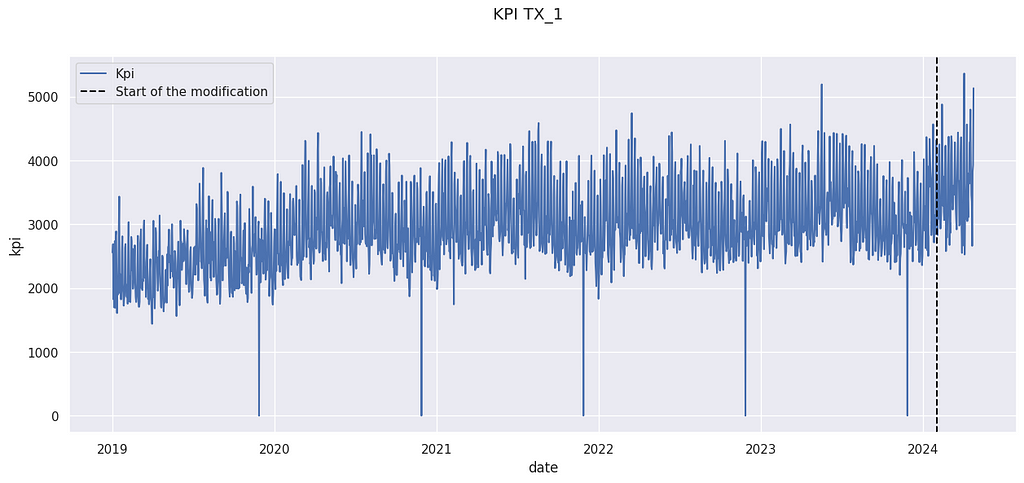
The above data come from the M5 Forecasting competition[3], but have been artificially modified. The details are postponed to the last section.

We have observed a KPI Yₜ on a store for a long period. An action has been taken on February 2024. For instance, it could have been the opening of a new competitor in the neighborhood, a new organization of the store, or a change in the pricing strategy. We want to know the impact of this modification.

Remark: This method does not work for punctual change, such as a marketing campaign. Google’s Causal Impact is more adapted in this case.

The proposed method

Let us sketch the method we will use to calculate the impact.

1- We will create a counterfactual prediction based on past data (before the modification). This counterfactual is based on classical ML techniques.

2- We will evaluate the performance of this predictor. This will allow us to compute confidence intervals and to ensure the validity of the use of its prediction.

3 -We will compare the prediction after the modification with the actual value. The prediction will represent what would have happened if the modification hadn’t occurred. Therefore, the difference between the actual value and the prediction is the uplift we measure.

Counterfactual Construction

We want to construct a counterfactual, i.e. a prediction noted Yₜ’ of the KPI Yₜ. There are many ways to construct a counterfactual. You use your favorite ML methods for time series forecasting. However, using classical time series techniques such as ARIMA to construct a counter-factual (a method called C-ARIMA [4]) is complex. Indeed, you cannot use data from after the modification to compute your counterfactual. Therefore, you will need to predict a long horizon with such techniques, and they are generally better ways to do so.

We will present here a simple solution when you have access to a control group. We consider that you have access to similar data not impacted by the modification. In our example, we will use data from other stores. It is therefore analog to a control group. This types of methodologies are called synthetic controls by economists[2], because it creates a synthetic control series instead of taking only one control time series.

X = X.assign(
    day_of_the_week =  X.reset_index().date.dt.isocalendar().day.values,
    trend = (X.reset_index().date- start_modification_date).dt.days.values
) 
X.head()

magasin  CA_1  TX_2  TX_3  WI_1  day_of_the_week  trend
date       
2019-01-01  4337  3852  3030  2704  2  0
2019-01-02  4155  3937  3006  2194  3  1
2019-01-03  2816  2731  2225  1562  4  2
2019-01-04  3051  2954  2169  1251  5  3
2019-01-05  2630  2492  1726    2  6  4

Here we use 4 stores (called CA_1, TX_2, TX_3 and WI_1) in our control features. We also use the day of the week and a trend indicator to train our model. The last one is very handy to limit time drift, which is the main weakness of the method presented in this article.

Note: WI_1 presents an outlier value on 2019–01–05. This is a typical explanation for why we want to have several stores in our control sets, instead of only choosing one store.

min_date =dt.datetime(2019,1,1)
K = 3 # Max order of the fourrier series
T= 365

x = [(i-min_date).days for i in X.index]
XX = np.array([([sin( 2 *k * pi * t /(T-1))for k in range(1, K+1)] +[cos( 2 * pi * k  * t /(T-1)) for k in range(1, K+1)] ) for t in x])
X = X.join(pd.DataFrame(XX,columns = [f'F_{i}' for i in range(2*K)], index = X.index))

We also add some features corresponding to Fourier coefficients. It is a known technique to integrate seasonalities into ML time series forecasts. It is not really necessary here, but it can improve your results if the data you have present strong seasonal behavior. You may replace them with classical B-spline functions.

Now, we have the features for our model. We will split our data into 3 sets:

1- Training dataset : It is the set of data where we will train our model

2 – Test dataset : Data used to evaluate the performance of our model.

3- After modification dataset: Data used to compute the uplift using our model.

from sklearn.model_selection import train_test_split

start_modification_date = dt.datetime(2024, 2,1)


X_before_modification = X[X.index < start_modification_date]
y_before_modification = y[y.index < start_modification_date].kpi
X_after_modification = X[X.index >= start_modification_date]
y_after_modification = y[y.index >= start_modification_date].kpi


X_train, X_test , y_train , y_test = train_test_split(X_before_modification, y_before_modification, test_size= 0.25, shuffle = False)

Note : You can use a fourth subset of data to perform some model selection. Here we won’t do a lot of model selection, so it does not matter a lot. But it will if you start to select your model among tenths of others.

Note 2: Cross-validation is also very possible and recommended.

Note 3 : I do recommend splitting data without shuffling (shuffling = False). It will allow you to be aware of the eventual temporal drift of your model.

from sklearn.ensemble import RandomForestRegressor


model = RandomForestRegressor(min_samples_split=4)
model.fit(X_train, y_train)
y_pred = model.predict(X_test)

And here you train your predictor. We use a random forest regressor for its convenience because it allows us to handle non-linearity, missing data, and outliers. Gradients Boosting Trees algorithms are also very good for this use.

Many papers about Synthetic Control will use linear regression here, but we think it is not useful here because we are not really interested in the model’s interpretability. Moreover, interpreting such regression can be tricky.

Counterfactual Evaluation

Our prediction will be on the testing set. The main hypothesis we will make is that the performance of the model will stay the same when we compute the uplift. That is why we tend to use a lot of data in our We consider 3 different key indicators to evaluate the quality of the counterfactual prediction :

1-Bias : Bias controls the presence of a gap between your counterfactual and the real data. It is a strong limit on your ability to compute because it won’t be reduced by waiting more time after the modification.

bias = float((y_pred -  y_test).mean()/(y_before_modification.mean()))
bias
> 0.0030433481322823257

We generally express the bias as a percentage of the average value of the KPI. It is smaller than 1%, so we should not expect to measure effects bigger than that. If your bias is too big, you should check for a temporal drift (and add a trend to your prediction). You can also correct your prediction and deduce the bias from the prediction, provided you control the effect of this correction of fresh data.

2-Standard Deviation σ: We also want to control how dispersed are the predictions around the true values. We therefore use the standard deviation, again expressed as a percentage of the average value of the kpi.

sigma = float((y_pred -  y_test).std()/(y_before_modification.mean()))
sigma
> 0.0780972738325956

The good news is that the uncertainty created by the deviation is reduced when the number of data points increase. We prefer a predictor without bias, so it could be necessary to accept an increase in the deviation if allowed to limit the bias.

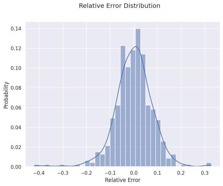
It can also be interesting to look at bias and variance by looking at the distribution of the forecasting errors. It can be useful to see if our calculation of bias and deviation is valid, or if it is affected by outliers and extreme values.

import seaborn as sns 
import matplotlib.pyplot as plt

f, ax = plt.subplots(figsize=(8, 6))
sns.histplot(pd.DataFrame((y_pred -  y_test)/y_past.mean()), x = 'kpi', bins = 35, kde = True, stat = 'probability')
f.suptitle('Relative Error Distribution')
ax.set_xlabel('Relative Error')
plt.show()

3- Auto-correlation α: In general, errors are auto-correlated. It means that if your prediction is above the true value on a given day, it has more chance of being above the next day. It is a problem because most classical statistical tools require independence between observations. What happened on a given day should affect the next one. We use auto-correlation as a measure of dependence between one day and the next.

df_test = pd.DataFrame(zip(y_pred, y_test), columns = ['Prevision','Real'], index = y_test.index)
df_test =  df_test.assign(
    ecart = df_test.Prevision - df_test.Real)
alpha = df_test.ecart.corr(df_test.ecart.shift(1))
alpha
> 0.24554635095548982

A high auto-correlation is problematic but can be managed. A possible causes for it are unobserved covariates. If for instance, the store you want to measure organized a special event, it could increase its sales for several days. This will lead to an unexpected sequence of days above the prevision.

df_test = pd.DataFrame(zip(y_pred, y_test), columns = ['Prevision','Reel'], index = y_test.index)

f, ax = plt.subplots(figsize=(15, 6))
sns.lineplot(data = df_test, x = 'date', y= 'Reel', label = 'True Value')
sns.lineplot(data = df_test, x = 'date', y= 'Prevision', label = 'Forecasted Value')
ax.axvline(start_modification_date, ls = '--', color = 'black', label = 'Start of the modification')
ax.legend()
f.suptitle('KPI TX_1')
plt.show()

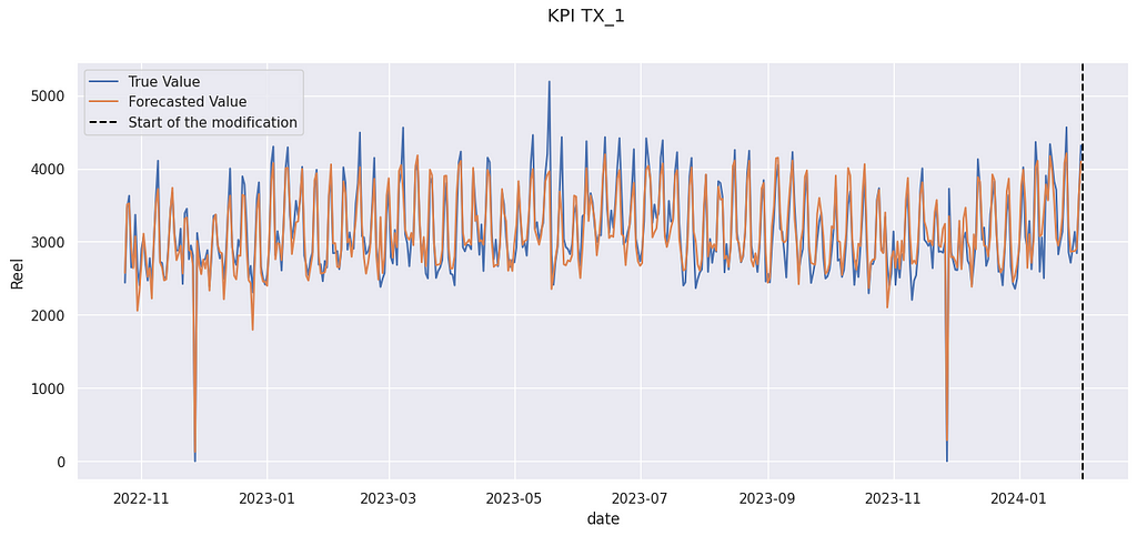
In the figure above, you can see an illustration of the auto-correlation phenomenon. In late April 2023, for several days, forecasted values are above the true value. Errors are not independent of one another.

Impact Calculation

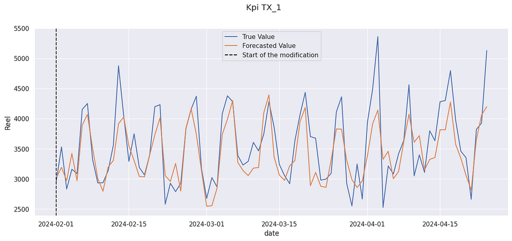
Now we can compute the impact of the modification. We compare the prediction after the modification with the actual value. As always, it is expressed as a percentage of the mean value of the KPI.

y_pred_after_modification = model.predict(X_after_modification)
uplift =float((y_after_modification - y_pred_after_modification).mean()/y_before_modification.mean())
uplift
> 0.04961773643584396

We get a relative increase of 4.9% The “true” value (the data used were artificially modified) was 3.0%, so we are not far from it. And indeed, the true value is often above the prediction :

We can compute a confidence interval for this value. If our predictor has no bias, the size of its confidence interval can be expressed with:

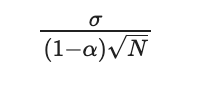
Where σ is the standard deviation of the prediction, α its auto-correlation, and N the number of days after the modification.

N = y_after_modification.shape[0]
ec = sigma/(sqrt(N) *(1-alpha))

print('68%% IC : [%.2f %% , %.2f %%]' % (100*(uplift - ec),100 * (uplift + ec) ))
print('95%% IC : [%.2f %% , %.2f %%]' % (100*(uplift -2 *ec),100 * (uplift +2*ec) ))

68% IC : [3.83 % , 6.09 %]
95% IC : [2.70 % , 7.22 %]

The range of the 95% CI is around 4.5% for 84 days. It is reasonable for many applications, because it is possible to run an experiment or a proof of concept for 3 months.

Note: the confidence interval is very sensitive to the deviation of the initial predictor. That is why it is a good idea to take some time to perform model selection (on the training set only) before selecting a good model.

Mathematical formulation of the model

So far we have tried to avoid maths, to allow for an easier comprehension. In this section, we will present the mathematical model beneath the model.

This model is very close to a classical i.i.d. forecasting error. The only difference is that the gap between the forecasted value and the true value follows a stationary AR(1) process. It allows for some auto-correlation to be taken into account.

We are doing the hypothesis is that there is no memory of the previous gap (as in a Markov chain), only a state transition. The knowledge of the current gap is enough to know the distribution of the gap for the next day.

Note: Other mathematical hypotheses (weak dependence ! contraction !) could have been made and will be more general. However, the impact of this hypothesis on the confidence interval will be small, and in practice, the main limitation of this method is the temporal drift, not the model of dependence between variables.

This model leads (with the help of the central limit theorem) to the confidence interval presented before.

Comparison with Causal Impact

Causal Impact is a methodology developed by several Google researchers to answer the general question of impact attribution. It does share some similarities with the model presented here. In particular, they also use a synthetic counterfactual created from several possible control values before the modification.

The main difference is that the model presented here is much more restrictive. The structural time-series model used by Causal allows for a variable impact, whereas we have assumed that this impact was constant. Moreover, seasonality and trend are directly modelized into the Causal Impact framework, which limits the temporal drift and the drawbacks of strong seasonality.

Another difference is that causal impacts allows for some modification on the construction of the synthetic control. It is indeed possible that the behavior of the covariates and the target variables change over time, creating a temporal drift. Causal Impact takes into account some possible modifications, reducing the risk of temporal drift, especially when N is large.

However, our models allow us to use powerful ML Techniques, which can be handy if we have only access to a noisy or partial control. Moreover, by using a tighter hypothesis, we are generally able to establish smaller confidence intervals.

Let’s try to use the Causal Impact models (using the tfp-causalimpact implementation). We use as control variables the 4 same stores as in our examples.

import causalimpact
from causalimpact import DataOptions
import altair as alt
alt.data_transformers.enable("vegafusion") # Useful to compute more than 5000 rows at time in Causal Impact

control = ['CA_1','TX_2', 'TX_3','WI_1']

data = X[control].assign(
    y = y.kpi.values /y.kpi.mean()
)
data = data.reset_index().drop(columns = 'date')


training_start = min(data.index)
training_end = X_before_modification.shape[0] - 1
treatment_start = X_before_modification.shape[0]
end_recording = max(data.index)

pre_period = [training_start, training_end]
post_period = [treatment_start, end_recording]

options = DataOptions()
options.outcome_column = 'y'

impact = causalimpact.fit_causalimpact(
    data=data,
    pre_period=pre_period,
    post_period=post_period,
    data_options=options
)
causalimpact.plot(impact)

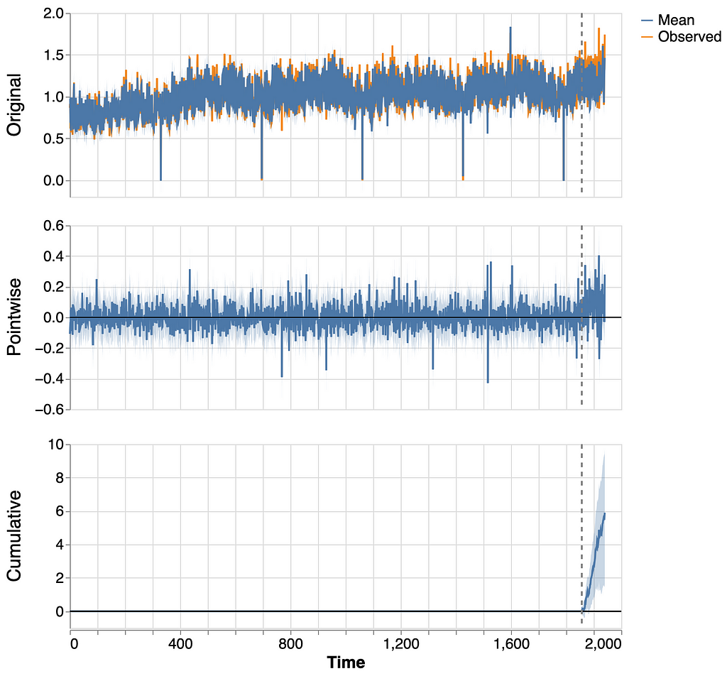
Causal effect observe a significant cumulative effect. Let us compute its statistics.

print(causalimpact.summary(impact, output_format='summary'))

Posterior Inference {CausalImpact}
                          Average            Cumulative
Actual                    1.2                101.7
Prediction (s.d.)         1.1 (0.02)         95.8 (2.05)
95% CI                    [1.1, 1.2]         [91.9, 100.0]

Absolute effect (s.d.)    0.1 (0.02)         5.9 (2.05)
95% CI                    [0.0, 0.1]         [1.7, 9.7]

Relative effect (s.d.)    6.2% (2.3%)        6.2% (2.0%)
95% CI                    [1.7%, 10.6%]      [1.7%, 10.6%]

Posterior tail-area probability p: 0.004
Posterior prob. of a causal effect: 99.56%

Causal Effect algorithm is also able to detect an effect, but it overestimates it ( 6.2% against the real 3%). Moreover, the range of the 95% CI is 9% (against 4.5% with our method), so it won’t be able to detect really small effects.

Conclusion

To sum up, our methodology works best :

• When we can suppose that the effect we want to measure is constant
• When available control data are noisy, or only partially avalaible
• When there is no trend in our prediction
• With fewer data points (due to the smaller IC)

Causal Impact will work best :

• When the effect we want to measure is not constant
• For times series with strong trend and/or seasonality patterns
• When we have a lot of data points (due to the risk of temporal drift)

Data Sources :

We used data from the M5 Forecasting competition[3]. The data comes from Walmart stores in three US States (California, Texas, and Wisconsin). We only use aggregated sales data from 5 stores :

• TX_1: our target store
• CA_1, TX_2, TX_3 and WI_1 : stores used to construct our synthetic control

The dates are completely fictitious and used mostly to have nice graphic representations.

data = pd.read_csv('sales_train_evaluation.csv')
set_stores = set(data.store_id)
df_list = []
for store in set_stores: 
    store_total = data[data.store_id == store].iloc[:, 6:].sum(axis= 0).reset_index()
    dates = [ dt.datetime(2019,1,1) +dt.timedelta(days =i) for i in range(1941)] 
    store_total = store_total.assign(magasin = store,date= dates )
    store_total.columns = ['dti','kpi', 'magasin', 'date']
    df_list.append(store_total)
df  = pd.concat(df_list)

target = 'TX_1'
control = ['CA_1','TX_2', 'TX_3','WI_1']


y = df[df.magasin == target].set_index('date')
X = df[df.magasin.isin(control)].set_index(['date','magasin']).kpi.unstack()

The target has been artificially modified to introduce a random uplift of mean 3%.

# Falsification :
 
start_modification_date = dt.datetime(2024, 2,1)
modif_value = 0.03
variance = 0.05

y = y.assign(
    random = lambda x: np.random.normal(loc = 1+ modif_value,scale = variance , size = y.shape[0] ), 
    kpi = lambda x :  x.kpi.where(x.index < start_modification_date, other = x.kpi * x.random)
)

Complete Code (without plots):

import pandas as pd 
import numpy as np
import datetime as dt
import seaborn as sns 
import matplotlib.pyplot as plt

from sklearn.model_selection import train_test_split
from sklearn.ensemble import RandomForestRegressor

sns.set_theme()

# Data 

data = pd.read_csv('sales_train_evaluation.csv')
set_stores = set(data.store_id)
df_list = []
for store in set_stores: 
    store_total = data[data.store_id == store].iloc[:, 6:].sum(axis= 0).reset_index()
    dates = [ dt.datetime(2019,1,1) +dt.timedelta(days =i) for i in range(1941)] 
    store_total = store_total.assign(magasin = store,date= dates )
    store_total.columns = ['dti','kpi', 'magasin', 'date']
    df_list.append(store_total)
df  = pd.concat(df_list)

target = 'TX_1'
control = ['CA_1','TX_2', 'TX_3','WI_1']

y = df[df.magasin == target].set_index('date')
X = df[df.magasin.isin(control)].set_index(['date','magasin']).kpi.unstack()

# Falsification :
 
start_modification_date = dt.datetime(2024, 2,1)
modif_value = 0.03
variance = 0.05

y = y.assign(
    random = lambda x: np.random.normal(loc = 1+ modif_value,scale = variance , size = y.shape[0] ), 
    kpi = lambda x :  x.kpi.where(x.index < start_modification_date, other = x.kpi * x.random)
)


# Features constructions
X = X.assign(
    day_of_the_week =  X.reset_index().date.dt.isocalendar().day.values,
    trend = (X.reset_index().date- start_modification_date).dt.days.values
)
min_date =dt.datetime(2019,1,1)
K = 3 # Max order of the fourrier series
T= 365
x = [(i-min_date).days for i in X.index]
XX = np.array([([sin( 2 *k * pi * t /(T-1))for k in range(1, K+1)] +[cos( 2 * pi * k  * t /(T-1)) for k in range(1, K+1)] ) for t in x])
X = X.join(pd.DataFrame(XX,columns = [f'F_{i}' for i in range(2*K)], index = X.index))


# Train/Test/AfterIntervention Split

start_modification_date = dt.datetime(2024, 2,1)
X_before_modification = X[X.index < start_modification_date]
y_before_modification = y[y.index < start_modification_date].kpi
X_after_modification = X[X.index >= start_modification_date]
y_after_modification = y[y.index >= start_modification_date].kpi

X_train, X_test , y_train , y_test = train_test_split(X_before_modification, y_before_modification, test_size= 0.25, shuffle = False)

# Model training

model = RandomForestRegressor(min_samples_split=4)
model.fit(X_train, y_train)
y_pred = model.predict(X_test)

# Model Evaluation

bias = float((y_pred -  y_test).mean()/(y_before_modification.mean()))
sigma = float((y_pred -  y_test).std()/(y_before_modification.mean()))
df_test = pd.DataFrame(zip(y_pred, y_test), columns = ['Prevision','Real'], index = y_test.index)
df_test =  df_test.assign(
    ecart = df_test.Prevision - df_test.Real)
alpha = df_test.ecart.corr(df_test.ecart.shift(1))

# Uplift Calculation

y_pred_after_modification = model.predict(X_after_modification)
uplift =float((y_after_modification - y_pred_after_modification).mean()/y_before_modification.mean())

N = y_after_modification.shape[0]
ec = sigma/(sqrt(N) *(1-alpha))

print('68%% IC : [%.2f %% , %.2f %%]' % (100*(uplift - ec),100 * (uplift + ec) ))
print('95%% IC : [%.2f %% , %.2f %%]' % (100*(uplift -2 *ec),100 * (uplift +2*ec) ))

References :

Unless otherwise noted, all images are by the author.

[1] Kay H. Brodersen. Fabian Gallusser. Jim Koehler. Nicolas Remy. Steven L. Scott., Inferring causal impact using Bayesian structural time-series models (2015), Ann. Appl. Stat.

[2] Matheus Facure Alves, Causal Inference for The Brave and True (2022)

[3] Addison Howard, inversion, Spyros Makridakis, and vangelis. M5 Forecasting — Accuracy. (2020) Kaggle.

[4] Robson Tigre , When and how to apply causal inference in time series (2024) Medium

The Data Scientist’s Dilemma: Answering “What If?” Questions Without Experiments was originally published in Towards Data Science on Medium, where people are continuing the conversation by highlighting and responding to this story.