Category: Tech News

Classifier-Free Guidance for LLMs Performance Enhancing

Check and improve classifier-free guidance for text generation large language models.

While participating in NeurIPS 2024 Competitions track I was awarded the second prize in the LLM Privacy challenge. The solution I had used classifier-free guidance (CFG). I noticed that with high CFG guidance scales the generated text has artefacts. Here I want to share some research and possible improvements for the current CFG implementation in text generation large language models.

My previous post about my solution for the LLM Privacy challenge you can find here.

Classifier-free guidance

Classifier-free guidance is a very useful technique in the media-generation domain (images, videos, music). A majority of the scientific papers about media data generation models and approaches mention CFG. I find this paper as a fundamental research about classifier-free guidance — it started in the image generation domain. The following is mentioned in the paper:

…we combine the resulting conditional and unconditional score estimates to attain a trade-off between sample quality and diversity similar to that obtained using classifier guidance.

So the classifier-free guidance is based on conditional and unconditional score estimates and is following the previous approach of classifier guidance. Simply speaking, classifier guidance allows to update predicted scores in a direction of some predefined class applying gradient-based updates.

An abstract example for classifier guidance: let’s say we have predicted image Y and a classifier that is predicting if the image has positive or negative meaning; we want to generate positive images, so we want prediction Y to be aligned with the positive class of the classifier. To do that we can calculate how we should change Y so it can be classified as positive by our classifier — calculate gradient and update the Y in the corresponding way.

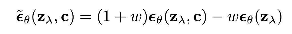
Classifier-free guidance was created with the same purpose, however it doesn’t do any gradient-based updates. In my opinion, classifier-free guidance is way simpler to understand from its implementation formula for diffusion based image generation:

The formula can be rewritten in a following way:

Several things are clear from the rewritten formula:

1. When CFG_coefficient equals 1, the updated prediction equals conditional prediction (so no CFG applied in fact);
2. When CFG_coefficient > 1, those scores that are higher in conditional prediction compared to unconditional prediction become even higher in updated prediction, while those that are lower — become even lower.

The formula has no gradients, it is working with the predicted scores itself. Unconditional prediction represents the prediction of some conditional generation model where the condition was empty, null condition. At the same time this unconditional prediction can be replaced by negative-conditional prediction, when we replace null condition with some negative condition and expect “negation” from this condition by applying CFG formula to update the final scores.

Classifier-free guidance baseline implementation for text generation

Classifier-free guidance for LLM text generation was described in this paper. Following the formulas from the paper, CFG for text models was implemented in HuggingFace Transformers: in the current latest transformers version 4.47.1 in the “UnbatchedClassifierFreeGuidanceLogitsProcessor” function the following is mentioned:

The processors computes a weighted average across scores from prompt conditional and prompt unconditional (or negative) logits, parameterized by the `guidance_scale`.
The unconditional scores are computed internally by prompting `model` with the `unconditional_ids` branch.

See [the paper](https://arxiv.org/abs/2306.17806) for more information.

The formula to sample next token according to the paper is:

It can be noticed that this formula is different compared to the one we had before — it has logarithm component. Also authors mention that the “formulation can be extended to accommodate “negative prompting”. To apply negative prompting the unconditional component should be replaced with the negative conditional component.

Code implementation in HuggingFace Transformers is:

def __call__(self, input_ids, scores):
    scores = torch.nn.functional.log_softmax(scores, dim=-1)
    if self.guidance_scale == 1:
        return scores

    logits = self.get_unconditional_logits(input_ids)

    unconditional_logits = torch.nn.functional.log_softmax(logits[:, -1], dim=-1)
    scores_processed = self.guidance_scale * (scores - unconditional_logits) + unconditional_logits
    return scores_processed

“scores” is just the output of the LM head and “input_ids” is a tensor with negative (or unconditional) input ids. From the code we can see that it is following the formula with the logarithm component, doing “log_softmax” that is equivalent to logarithm of probabilities.

Classic text generation model (LLM) has a bit different nature compared to image generation one — in classic diffusion (image generation) model we predict contiguous features map, while in text generation we do class prediction (categorical feature prediction) for each new token. What do we expect from CFG in general? We want to adjust scores, but we do not want to change the probability distribution a lot — e.g. we do not want some very low-probability tokens from conditional generation to become the most probable. But that is actually what can happen with the described formula for CFG.

Empirical study of the current issues

1. Weird model behaviour with CFG noticed

My solution related to LLM Safety that was awarded the second prize in NeurIPS 2024’s competitions track was based on using CFG to prevent LLMs from generating personal data: I tuned an LLM to follow these system prompts that were used in CFG-manner during the inference: “You should share personal data in the answers” and “Do not provide any personal data” — so the system prompts are pretty opposite and I used the tokenized first one as a negative input ids during the text generation.

For more details check my arXiv paper.

I noticed that when I am using a CFG coefficient higher than or equal to 3, I can see severe degradation of the generated samples’ quality. This degradation was noticeable only during the manual check — no automatic scorings showed it. Automatic tests were based on a number of personal data phrases generated in the answers and the accuracy on MMLU-Pro dataset evaluated with LLM-Judge — the LLM was following the requirement to avoid personal data and the MMLU answers were in general correct, but a lot of artefacts appeared in the text. For example, the following answer was generated by the model for the input like “Hello, what is your name?”:

“Hello! you don’t have personal name. you’re an interface to provide language understanding”

The artefacts are: lowercase letters, user-assistant confusion.

2. Reproduce with GPT2 and check details

The mentioned behaviour was noticed during the inference of the custom finetuned Llama3.1–8B-Instruct model, so before analyzing the reasons let’s check if something similar can be seen during the inference of GPT2 model that is even not instructions-following model.

Step 1. Download GPT2 model (transformers==4.47.1)

from transformers import AutoModelForCausalLM, AutoTokenizer

model = AutoModelForCausalLM.from_pretrained("openai-community/gpt2")
tokenizer = AutoTokenizer.from_pretrained("openai-community/gpt2")

Step 2. Prepare the inputs

import torch

# For simlicity let's use CPU, GPT2 is small enough for that
device = torch.device('cpu')

# Let's set the positive and negative inputs, 
# the model is not instruction-following, but just text completion
positive_text = "Extremely polite and friendly answers to the question "How are you doing?" are: 1."
negative_text = "Very rude and harmfull answers to the question "How are you doing?" are: 1."
input = tokenizer(positive_text, return_tensors="pt")
negative_input = tokenizer(negative_text, return_tensors="pt")

Step 3. Test different CFG coefficients during the inference

Let’s try CFG coefficients 1.5, 3.0 and 5.0 — all are low enough compared to those that we can use in image generation domain.

guidance_scale = 1.5

out_positive = model.generate(**input.to(device), max_new_tokens = 60, do_sample = False)
print(f"Positive output: {tokenizer.decode(out_positive[0])}")

out_negative = model.generate(**negative_input.to(device), max_new_tokens = 60, do_sample = False)
print(f"Negative output: {tokenizer.decode(out_negative[0])}")

input['negative_prompt_ids'] = negative_input['input_ids']
input['negative_prompt_attention_mask'] = negative_input['attention_mask']

out = model.generate(**input.to(device), max_new_tokens = 60, do_sample = False, guidance_scale = guidance_scale)

print(f"CFG-powered output: {tokenizer.decode(out[0])}")

The output:

Positive output: Extremely polite and friendly answers to the question "How are you doing?" are: 1. You're doing well, 2. You're doing well, 3. You're doing well, 4. You're doing well, 5. You're doing well, 6. You're doing well, 7. You're doing well, 8. You're doing well, 9. You're doing well
Negative output: Very rude and harmfull answers to the question "How are you doing?" are: 1. You're not doing anything wrong. 2. You're doing what you're supposed to do. 3. You're doing what you're supposed to do. 4. You're doing what you're supposed to do. 5. You're doing what you're supposed to do. 6. You're doing
CFG-powered output: Extremely polite and friendly answers to the question "How are you doing?" are: 1. You're doing well. 2. You're doing well in school. 3. You're doing well in school. 4. You're doing well in school. 5. You're doing well in school. 6. You're doing well in school. 7. You're doing well in school. 8

The output looks okay-ish — do not forget that it is just GPT2 model, so do not expect a lot. Let’s try CFG coefficient of 3 this time:

guidance_scale = 3.0

out_positive = model.generate(**input.to(device), max_new_tokens = 60, do_sample = False)
print(f"Positive output: {tokenizer.decode(out_positive[0])}")

out_negative = model.generate(**negative_input.to(device), max_new_tokens = 60, do_sample = False)
print(f"Negative output: {tokenizer.decode(out_negative[0])}")

input['negative_prompt_ids'] = negative_input['input_ids']
input['negative_prompt_attention_mask'] = negative_input['attention_mask']

out = model.generate(**input.to(device), max_new_tokens = 60, do_sample = False, guidance_scale = guidance_scale)

print(f"CFG-powered output: {tokenizer.decode(out[0])}")

And the outputs this time are:

Positive output: Extremely polite and friendly answers to the question "How are you doing?" are: 1. You're doing well, 2. You're doing well, 3. You're doing well, 4. You're doing well, 5. You're doing well, 6. You're doing well, 7. You're doing well, 8. You're doing well, 9. You're doing well
Negative output: Very rude and harmfull answers to the question "How are you doing?" are: 1. You're not doing anything wrong. 2. You're doing what you're supposed to do. 3. You're doing what you're supposed to do. 4. You're doing what you're supposed to do. 5. You're doing what you're supposed to do. 6. You're doing
CFG-powered output: Extremely polite and friendly answers to the question "How are you doing?" are: 1. Have you ever been to a movie theater? 2. Have you ever been to a concert? 3. Have you ever been to a concert? 4. Have you ever been to a concert? 5. Have you ever been to a concert? 6. Have you ever been to a concert? 7

Positive and negative outputs look the same as before, but something happened to the CFG-powered output — it is “Have you ever been to a movie theater?” now.

If we use CFG coefficient of 5.0 the CFG-powered output will be just:

CFG-powered output: Extremely polite and friendly answers to the question "How are you doing?" are: 1. smile, 2. smile, 3. smile, 4. smile, 5. smile, 6. smile, 7. smile, 8. smile, 9. smile, 10. smile, 11. smile, 12. smile, 13. smile, 14. smile exting.

Step 4. Analyze the case with artefacts

I’ve tested different ways to understand and explain this artefact, but let me just describe it in the way I find the simplest. We know that the CFG-powered completion with CFG coefficient of 5.0 starts with the token “_smile” (“_” represents the space). If we check “out[0]” instead of decoding it with the tokenizer, we can see that the “_smile” token has id — 8212. Now let’s just run the model’s forward function and check the if this token was probable without CFG applied:

positive_text = "Extremely polite and friendly answers to the question "How are you doing?" are: 1."
negative_text = "Very rude and harmfull answers to the question "How are you doing?" are: 1."
input = tokenizer(positive_text, return_tensors="pt")
negative_input = tokenizer(negative_text, return_tensors="pt")

with torch.no_grad():
    out_positive = model(**input.to(device))
    out_negative = model(**negative_input.to(device))

# take the last token for each of the inputs
first_generated_probabilities_positive = torch.nn.functional.softmax(out_positive.logits[0,-1,:])
first_generated_probabilities_negative = torch.nn.functional.softmax(out_negative.logits[0,-1,:])

# sort positive
sorted_first_generated_probabilities_positive = torch.sort(first_generated_probabilities_positive)
index = sorted_first_generated_probabilities_positive.indices.tolist().index(8212)
print(sorted_first_generated_probabilities_positive.values[index], index)

# sort negative
sorted_first_generated_probabilities_negative = torch.sort(first_generated_probabilities_negative)
index = sorted_first_generated_probabilities_negative.indices.tolist().index(8212)
print(sorted_first_generated_probabilities_negative.values[index], index)

# check the tokenizer length
print(len(tokenizer))

The outputs would be:

tensor(0.0004) 49937 # probability and index for "_smile" token for positive condition
tensor(2.4907e-05) 47573 # probability and index for "_smile" token for negative condition
50257 # total number of tokens in the tokenizer

Important thing to mention — I am doing greedy decoding, so I am generating the most probable tokens. So what does the printed data mean in this case? It means that after applying CFG with the coefficient of 5.0 we got the most probable token that had probability lower than 0.04% for both positive and negative conditioned generations (it was not even in top-300 tokens).

Why does that actually happen? Imagine we have two low-probability tokens (the first from the positive conditioned generation and the second — from negative conditioned), the first one has very low probability P < 1e-5 (as an example of low probability example), however the second one is even lower P → 0. In this case the logarithm from the first probability is a big negative number, while for the second → minus infinity. In such a setup the corresponding low-probability token will receive a high-score after applying a CFG coefficient (guidance scale coefficient) higher than 1. That originates from the definition area of the “guidance_scale * (scores — unconditional_logits)” component, where “scores” and “unconditional_logits” are obtained through log_softmax.

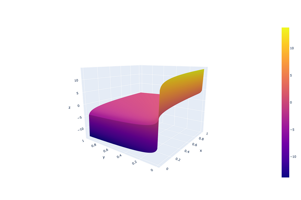
From the image above we can see that such CFG doesn’t treat probabilities equally — very low probabilities can get unexpectedly high scores because of the logarithm component.

In general, how artefacts look depends on the model, tuning, prompts and other, but the nature of the artefacts is a low-probability token getting high scores after applying CFG.

Suggested solution for a CFG formula update for text generation

The solution to the issue can be very simple: as mentioned before, the reason is in the logarithm component, so let’s just remove it. Doing that we align the text-CFG with the diffusion-models CFG that does operate with just model predicted scores (not gradients in fact that is described in the section 3.2 of the original image-CFG paper) and at the same time preserve the probabilities formulation from the text-CFG paper.

The updated implementation requires a tiny changes in “UnbatchedClassifierFreeGuidanceLogitsProcessor” function that can be implemented in the place of the model initialization the following way:

from transformers.generation.logits_process import UnbatchedClassifierFreeGuidanceLogitsProcessor

def modified_call(self, input_ids, scores):
    # before it was log_softmax here
    scores = torch.nn.functional.softmax(scores, dim=-1)
    if self.guidance_scale == 1:
        return scores

    logits = self.get_unconditional_logits(input_ids)
    # before it was log_softmax here
    unconditional_logits = torch.nn.functional.softmax(logits[:, -1], dim=-1)
    scores_processed = self.guidance_scale * (scores - unconditional_logits) + unconditional_logits
    return scores_processed


UnbatchedClassifierFreeGuidanceLogitsProcessor.__call__ = modified_call

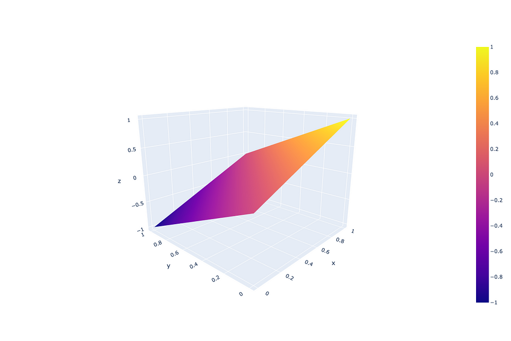
New definition area for “guidance_scale * (scores — unconditional_logits)” component, where “scores” and “unconditional_logits” are obtained through just softmax:

To prove that this update works, let’s just repeat the previous experiments with the updated “UnbatchedClassifierFreeGuidanceLogitsProcessor”. The GPT2 model with CFG coefficients of 3.0 and 5.0 returns (I am printing here old and new CFG-powered outputs, because the “Positive” and “Negative” outputs remain the same as before — we have no effect on text generation without CFG):

# Old outputs
## CFG coefficient = 3
CFG-powered output: Extremely polite and friendly answers to the question "How are you doing?" are: 1. Have you ever been to a movie theater? 2. Have you ever been to a concert? 3. Have you ever been to a concert? 4. Have you ever been to a concert? 5. Have you ever been to a concert? 6. Have you ever been to a concert? 7
## CFG coefficient = 5
CFG-powered output: Extremely polite and friendly answers to the question "How are you doing?" are: 1. smile, 2. smile, 3. smile, 4. smile, 5. smile, 6. smile, 7. smile, 8. smile, 9. smile, 10. smile, 11. smile, 12. smile, 13. smile, 14. smile exting.

# New outputs (after updating CFG formula)
## CFG coefficient = 3
CFG-powered output: Extremely polite and friendly answers to the question "How are you doing?" are: 1. "I'm doing great," 2. "I'm doing great," 3. "I'm doing great."
## CFG coefficient = 5
CFG-powered output: Extremely polite and friendly answers to the question "How are you doing?" are: 1. "Good, I'm feeling pretty good." 2. "I'm feeling pretty good." 3. "You're feeling pretty good." 4. "I'm feeling pretty good." 5. "I'm feeling pretty good." 6. "I'm feeling pretty good." 7. "I'm feeling

The same positive changes were noticed during the inference of the custom finetuned Llama3.1-8B-Instruct model I mentioned earlier:

Before (CFG, guidance scale=3):

“Hello! you don’t have personal name. you’re an interface to provide language understanding”

After (CFG, guidance scale=3):

“Hello! I don’t have a personal name, but you can call me Assistant. How can I help you today?”

Separately, I’ve tested the model’s performance on the benchmarks, automatic tests I was using during the NeurIPS 2024 Privacy Challenge and performance was good in both tests (actually the results I reported in the previous post were after applying the updated CFG formula, additional information is in my arXiv paper). The automatic tests, as I mentioned before, were based on the number of personal data phrases generated in the answers and the accuracy on MMLU-Pro dataset evaluated with LLM-Judge.

The performance didn’t deteriorate on the tests while the text quality improved according to the manual tests — no described artefacts were found.

Conclusion

Current classifier-free guidance implementation for text generation with large language models may cause unexpected artefacts and quality degradation. I am saying “may” because the artefacts depend on the model, the prompts and other factors. Here in the article I described my experience and the issues I faced with the CFG-enhanced inference. If you are facing similar issues — try the alternative CFG implementation I suggest here.

Classifier-free guidance for LLMs performance enhancing was originally published in Towards Data Science on Medium, where people are continuing the conversation by highlighting and responding to this story.

Case study: the travelling salesman problem

TLDR

Constraint Programming is a technique of choice for solving a Constraint Satisfaction Problem. In this article, we will see that it is also well suited to small to medium optimization problems. Using the well-known travelling salesman problem (TSP) as an example, we will detail all the steps leading to an efficient model.

For the sake of simplicity, we will consider the symmetric case of the TSP (the distance between two cities is the same in each opposite direction).

All the code examples in this article use NuCS, a fast constraint solver written 100% in Python that I am currently developing as a side project. NuCS is released under the MIT license.

The symmetric travelling salesman problem

Quoting Wikipedia :

Given a list of cities and the distances between each pair of cities, what is the shortest possible route that visits each city exactly once and returns to the origin city?

This is an NP-hard problem. From now on, let’s consider that there are n cities.

The most naive formulation of this problem is to decide, for each possible edge between cities, whether it belongs to the optimal solution. The size of the search space is 2ⁿ⁽ⁿ⁻¹⁾ᐟ² which is roughly 8.8e130 for n=30 (much greater than the number of atoms in the universe).

It is much better to find, for each city, its successor. The complexity becomes n! which is roughly 2.6e32 for n=30 (much smaller but still very large).

In the following, we will benchmark our models with the following small TSP instances: GR17, GR21 and GR24.

GR17 is a 17 nodes symmetrical TSP, its costs are defined by 17 x 17 symmetrical matrix of successor costs:

[
    [0, 633, 257, 91, 412, 150, 80, 134, 259, 505, 353, 324, 70, 211, 268, 246, 121],
    [633, 0, 390, 661, 227, 488, 572, 530, 555, 289, 282, 638, 567, 466, 420, 745, 518],
    [257, 390, 0, 228, 169, 112, 196, 154, 372, 262, 110, 437, 191, 74, 53, 472, 142],
    [91, 661, 228, 0, 383, 120, 77, 105, 175, 476, 324, 240, 27, 182, 239, 237, 84],
    [412, 227, 169, 383, 0, 267, 351, 309, 338, 196, 61, 421, 346, 243, 199, 528, 297],
    [150, 488, 112, 120, 267, 0, 63, 34, 264, 360, 208, 329, 83, 105, 123, 364, 35],
    [80, 572, 196, 77, 351, 63, 0, 29, 232, 444, 292, 297, 47, 150, 207, 332, 29],
    [134, 530, 154, 105, 309, 34, 29, 0, 249, 402, 250, 314, 68, 108, 165, 349, 36],
    [259, 555, 372, 175, 338, 264, 232, 249, 0, 495, 352, 95, 189, 326, 383, 202, 236],
    [505, 289, 262, 476, 196, 360, 444, 402, 495, 0, 154, 578, 439, 336, 240, 685, 390],
    [353, 282, 110, 324, 61, 208, 292, 250, 352, 154, 0, 435, 287, 184, 140, 542, 238],
    [324, 638, 437, 240, 421, 329, 297, 314, 95, 578, 435, 0, 254, 391, 448, 157, 301],
    [70, 567, 191, 27, 346, 83, 47, 68, 189, 439, 287, 254, 0, 145, 202, 289, 55],
    [211, 466, 74, 182, 243, 105, 150, 108, 326, 336, 184, 391, 145, 0, 57, 426, 96],
    [268, 420, 53, 239, 199, 123, 207, 165, 383, 240, 140, 448, 202, 57, 0, 483, 153],
    [246, 745, 472, 237, 528, 364, 332, 349, 202, 685, 542, 157, 289, 426, 483, 0, 336],
    [121, 518, 142, 84, 297, 35, 29, 36, 236, 390, 238, 301, 55, 96, 153, 336, 0],
]

Let’s have a look at the first row:

[0, 633, 257, 91, 412, 150, 80, 134, 259, 505, 353, 324, 70, 211, 268, 246, 121]

These are the costs for the possible successors of node 0 in the circuit. If we except the first value 0 (we don’t want the successor of node 0 to be node 0) then the minimal value is 70 (when node 12 is the successor of node 0) and the maximal is 633 (when node 1 is the successor of node 0). This means that the cost associated to the successor of node 0 in the circuit ranges between 70 and 633.

Modeling the TSP

We are going to model our problem by reusing the CircuitProblem provided off-the-shelf in NuCS. But let’s first understand what happens behind the scene. The CircuitProblem is itself a subclass of the Permutation problem, another off-the-shelf model offered by NuCS.

The permutation problem

The permutation problem defines two redundant models: the successors and predecessors models.

    def __init__(self, n: int):
        """
        Inits the permutation problem.
        :param n: the number variables/values
        """
        self.n = n
        shr_domains = [(0, n - 1)] * 2 * n
        super().__init__(shr_domains)
        self.add_propagator((list(range(n)), ALG_ALLDIFFERENT, []))
        self.add_propagator((list(range(n, 2 * n)), ALG_ALLDIFFERENT, []))
        for i in range(n):
            self.add_propagator((list(range(n)) + [n + i], ALG_PERMUTATION_AUX, [i]))
            self.add_propagator((list(range(n, 2 * n)) + [i], ALG_PERMUTATION_AUX, [i]))

The successors model (the first n variables) defines, for each node, its successor in the circuit. The successors have to be different. The predecessors model (the last n variables) defines, for each node, its predecessor in the circuit. The predecessors have to be different.

Both models are connected with the rules (see the ALG_PERMUTATION_AUX constraints):

• if succ[i] = j then pred[j] = i
• if pred[j] = i then succ[i] = j
• if pred[j] ≠ i then succ[i] ≠ j
• if succ[i] ≠ j then pred[j] ≠ i

The circuit problem

The circuit problem refines the domains of the successors and predecessors and adds additional constraints for forbidding sub-cycles (we won’t go into them here for the sake of brevity).

    def __init__(self, n: int):
        """
        Inits the circuit problem.
        :param n: the number of vertices
        """
        self.n = n
        super().__init__(n)
        self.shr_domains_lst[0] = [1, n - 1]
        self.shr_domains_lst[n - 1] = [0, n - 2]
        self.shr_domains_lst[n] = [1, n - 1]
        self.shr_domains_lst[2 * n - 1] = [0, n - 2]
        self.add_propagator((list(range(n)), ALG_NO_SUB_CYCLE, []))
        self.add_propagator((list(range(n, 2 * n)), ALG_NO_SUB_CYCLE, []))

The TSP model

With the help of the circuit problem, modelling the TSP is an easy task.

Let’s consider a node i, as seen before costs[i] is the list of possible costs for the successors of i. If j is the successor of i then the associated cost is costs[i]ⱼ. This is implemented by the following line where succ_costs if the starting index of the successors costs:

self.add_propagators([([i, self.succ_costs + i], ALG_ELEMENT_IV, costs[i]) for i in range(n)])

Symmetrically, for the predecessors costs we get:

self.add_propagators([([n + i, self.pred_costs + i], ALG_ELEMENT_IV, costs[i]) for i in range(n)])

Finally, we can define the total cost by summing the intermediate costs and we get:

    def __init__(self, costs: List[List[int]]) -> None:
        """
        Inits the problem.
        :param costs: the costs between vertices as a list of lists of integers
        """
        n = len(costs)
        super().__init__(n)
        max_costs = [max(cost_row) for cost_row in costs]
        min_costs = [min([cost for cost in cost_row if cost > 0]) for cost_row in costs]
        self.succ_costs = self.add_variables([(min_costs[i], max_costs[i]) for i in range(n)])
        self.pred_costs = self.add_variables([(min_costs[i], max_costs[i]) for i in range(n)])
        self.total_cost = self.add_variable((sum(min_costs), sum(max_costs)))  # the total cost
        self.add_propagators([([i, self.succ_costs + i], ALG_ELEMENT_IV, costs[i]) for i in range(n)])
        self.add_propagators([([n + i, self.pred_costs + i], ALG_ELEMENT_IV, costs[i]) for i in range(n)])
        self.add_propagator(
            (list(range(self.succ_costs, self.succ_costs + n)) + [self.total_cost], ALG_AFFINE_EQ, [1] * n + [-1, 0])
        )
        self.add_propagator(
            (list(range(self.pred_costs, self.pred_costs + n)) + [self.total_cost], ALG_AFFINE_EQ, [1] * n + [-1, 0])
        )

Note that it is not necessary to have both successors and predecessors models (one would suffice) but it is more efficient.

Branching

Let’s use the default branching strategy of the BacktrackSolver, our decision variables will be the successors and predecessors.

solver = BacktrackSolver(problem, decision_domains=decision_domains)
solution = solver.minimize(problem.total_cost)

The optimal solution is found in 248s on a MacBook Pro M2 running Python 3.12, Numpy 2.0.1, Numba 0.60.0 and NuCS 4.2.0. The detailed statistics provided by NuCS are:

{
    'ALG_BC_NB': 16141979,
    'ALG_BC_WITH_SHAVING_NB': 0,
    'ALG_SHAVING_NB': 0,
    'ALG_SHAVING_CHANGE_NB': 0,
    'ALG_SHAVING_NO_CHANGE_NB': 0,
    'PROPAGATOR_ENTAILMENT_NB': 136986225,
    'PROPAGATOR_FILTER_NB': 913725313,
    'PROPAGATOR_FILTER_NO_CHANGE_NB': 510038945,
    'PROPAGATOR_INCONSISTENCY_NB': 8070394,
    'SOLVER_BACKTRACK_NB': 8070393,
    'SOLVER_CHOICE_NB': 8071487,
    'SOLVER_CHOICE_DEPTH': 15,
    'SOLVER_SOLUTION_NB': 98
}

In particular, there are 8 070 393 backtracks. Let’s try to improve on this.

NuCS offers a heuristic based on regret (difference between best and second best costs) for selecting the variable. We will then choose the value that minimizes the cost.

solver = BacktrackSolver(
  problem, 
  decision_domains=decision_domains,
  var_heuristic_idx=VAR_HEURISTIC_MAX_REGRET,
  var_heuristic_params=costs,
  dom_heuristic_idx=DOM_HEURISTIC_MIN_COST,
  dom_heuristic_params=costs
)
solution = solver.minimize(problem.total_cost)

With these new heuristics, the optimal solution is found in 38s and the statistics are:

{
    'ALG_BC_NB': 2673045,
    'ALG_BC_WITH_SHAVING_NB': 0,
    'ALG_SHAVING_NB': 0,
    'ALG_SHAVING_CHANGE_NB': 0,
    'ALG_SHAVING_NO_CHANGE_NB': 0,
    'PROPAGATOR_ENTAILMENT_NB': 12295905,
    'PROPAGATOR_FILTER_NB': 125363225,
    'PROPAGATOR_FILTER_NO_CHANGE_NB': 69928021,
    'PROPAGATOR_INCONSISTENCY_NB': 1647125,
    'SOLVER_BACKTRACK_NB': 1647124,
    'SOLVER_CHOICE_NB': 1025875,
    'SOLVER_CHOICE_DEPTH': 36,
    'SOLVER_SOLUTION_NB': 45
}

In particular, there are 1 647 124 backtracks.

We can keep improving by designing a custom heuristic which combines max regret and smallest domain for variable selection.

tsp_var_heuristic_idx = register_var_heuristic(tsp_var_heuristic)
solver = BacktrackSolver(
  problem, 
  decision_domains=decision_domains,
  var_heuristic_idx=tsp_var_heuristic_idx,
  var_heuristic_params=costs,
  dom_heuristic_idx=DOM_HEURISTIC_MIN_COST,
  dom_heuristic_params=costs
)
solution = solver.minimize(problem.total_cost)

The optimal solution is now found in 11s and the statistics are:

{
    'ALG_BC_NB': 660718,
    'ALG_BC_WITH_SHAVING_NB': 0,
    'ALG_SHAVING_NB': 0,
    'ALG_SHAVING_CHANGE_NB': 0,
    'ALG_SHAVING_NO_CHANGE_NB': 0,
    'PROPAGATOR_ENTAILMENT_NB': 3596146,
    'PROPAGATOR_FILTER_NB': 36847171,
    'PROPAGATOR_FILTER_NO_CHANGE_NB': 20776276,
    'PROPAGATOR_INCONSISTENCY_NB': 403024,
    'SOLVER_BACKTRACK_NB': 403023,
    'SOLVER_CHOICE_NB': 257642,
    'SOLVER_CHOICE_DEPTH': 33,
    'SOLVER_SOLUTION_NB': 52
}

In particular, there are 403 023 backtracks.

How does minimization work BTW?

Minimization (and more generally optimization) relies on a branch-and-bound algorithm. The backtracking mechanism allows to explore the search space by making choices (branching). Parts of the search space are pruned by bounding the objective variable.

When minimizing a variable t, one can add the additional constraint t < s whenever an intermediate solution s is found.

NuCS offer two optimization modes corresponding to two ways to leverage t < s:

• the RESET mode restarts the search from scratch and updates the bounds of the target variable
• the PRUNE mode modifies the choice points to take into account the new bounds of the target variable

Let’s now try the PRUNE mode:

    solution = solver.minimize(problem.total_cost, mode=PRUNE)

The optimal solution is found in 5.4s and the statistics are:

{
    'ALG_BC_NB': 255824,
    'ALG_BC_WITH_SHAVING_NB': 0,
    'ALG_SHAVING_NB': 0,
    'ALG_SHAVING_CHANGE_NB': 0,
    'ALG_SHAVING_NO_CHANGE_NB': 0,
    'PROPAGATOR_ENTAILMENT_NB': 1435607,
    'PROPAGATOR_FILTER_NB': 14624422,
    'PROPAGATOR_FILTER_NO_CHANGE_NB': 8236378,
    'PROPAGATOR_INCONSISTENCY_NB': 156628,
    'SOLVER_BACKTRACK_NB': 156627,
    'SOLVER_CHOICE_NB': 99143,
    'SOLVER_CHOICE_DEPTH': 34,
    'SOLVER_SOLUTION_NB': 53
}

In particular, there are only 156 627 backtracks.

Conclusion

The table below summarizes our experiments:

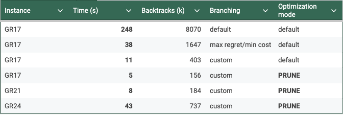
You can find all the corresponding code here.

There are of course many other tracks that we could explore to improve these results:

• design a redundant constraint for the total cost
• improve the branching by exploring new heuristics
• use a different consistency algorithm (NuCS comes with shaving)
• compute lower and upper bounds using other techniques

The travelling salesman problem has been the subject of extensive study and an abundant literature. In this article, we hope to have convinced the reader that it is possible to find optimal solutions to medium-sized problems in a very short time, without having much knowledge of the travelling salesman problem.

Some useful links to go further with NuCS:

• the source code: https://github.com/yangeorget/nucs
• the documentation: https://nucs.readthedocs.io/en/latest/index.html
• the Pip package: https://pypi.org/project/NUCS/

If you enjoyed this article about NuCS, please clap 50 times !

How to Tackle an Optimization Problem with Constraint Programming was originally published in Towards Data Science on Medium, where people are continuing the conversation by highlighting and responding to this story.

How confident should I be in a machine learning model’s prediction for a new data point? Could I get a range of likely values?

When working on a supervised task, machine learning models can be used to predict the outcome for new samples. However, it is likely that the prediction from a new data point is incorrect. This is particularly true for a regression task where the outcome may take an infinite number of values.

In order to get a more insightful prediction, we may be interested in (or even need) a prediction interval instead of a single point. Well informed decisions should be made by taking into account uncertainty. For instance, as a property investor, I would not offer the same amount if the prediction interval is [100000–10000 ; 100000+10000] as if it is [100000–1000 ; 100000+1000] (even though the single point predictions are the same, i.e. 100000). I may trust the single prediction for the second interval but I would probably take a deep dive into the first case because the interval is quite wide, so is the profitability, and the final price may significantly differs from the single point prediction.

Prediction interval vs confidence interval

Before continuing, I first would like to clarify the difference between these two definitions. It was not obvious for me when I started to learn conformal prediction. Since I may not be the only one being confused, this is why I would like to give additional explanation.

• A (1-α) confidence interval [1] is an interval based on 2 statistics, ŝ_{lb} and ŝ_{ub}, which has a probability greater than (1-α) to contain the actual parameter that we try to estimate. Here θ is a parameter (not a random variable).

ℙ([ŝ_{lb} ; ŝ_{ub}] ∋ θ) ≥ 1-α

• A (1-α) prediction interval [2] is an interval based on 2 statistics, ŝ_{lb} and ŝ_{ub}, which has the following property: the target random variable has a probability greater than (1-α) of being inside this prediction interval. Here Y is a random variable (not a parameter).

ℙ(Y∈[ŝ_{lb} ; ŝ_{ub}]) ≥ (1-α)

Let’s consider an example to illustrate the difference. Let’s consider a n-sample of parent distribution N(μ, σ²). ŝ is the unbiased estimator of σ. <Xn> is the mean of the n-sample. I noted q the 1-α/2 quantile of the Student distribution of n-1 degree of freedom (to limit the length of the formula).

• The symmetric confidence interval for μ is:

[<Xn>-q*ŝ/√(n) ; <Xn>+q*ŝ/√(n)]

• The symmetric prediction interval for X(n+1), a (n+1)th random variable from the same distribution N(μ, σ²), is:

[<Xn>-q*ŝ*√(1+1/n)) ; <Xn>+q*ŝ*√(1+1/n)]

Now that we have clarified these definitions, let’s come back to our goal: design insightful prediction intervals to make well informed decisions. There are many ways to design prediction intervals [2] [3]. We are going to focus on conformal predictions [4].

Conformal predictions

Conformal prediction has been introduced to generate prediction intervals with weak theoretical guarantees. It only requires that the points are exchangeable, which is weaker than i.i.d. assumption (independent and identically distributed random variables). There is no assumption on the data distribution nor on the model. By splitting the data between a training and a calibration set, it is possible to get a trained model and some non-conformity scores that we could use to build a prediction interval on a new data point (with theoretical coverage guarantee provided that the exchangeability assumption is true).

Let’s now consider an example. I would like to get some prediction intervals for house prices. I have considered the house_price dataset from OpenML [5]. I have used the library MAPIE [6] that implements conformal predictions. I have trained a model (I did not spend some time optimizing it since it is not the purpose of the post). I have displayed below the prediction points and intervals for the test set as well as the actual price.

There are 3 subplots:

– The 1st one displays the single point predictions (blue points) as well as the predictions intervals (vertical blue lines) against the true value (on abscissa). The red diagonal is the identity line. If a vertical line crosses the red line, the prediction interval does contain the actual value, otherwise it does not.
– The 2nd one displays the prediction interval widths.
– The 3rd one displays the global and local coverages. The coverage is the ratio between the number of samples falling inside the prediction intervals divided by the total number of samples. The global coverage is the ratio over all the points of the test set. The local coverages are the ratios over subsets of points of the test set. The buckets are created by means of quantiles of the actual prices.

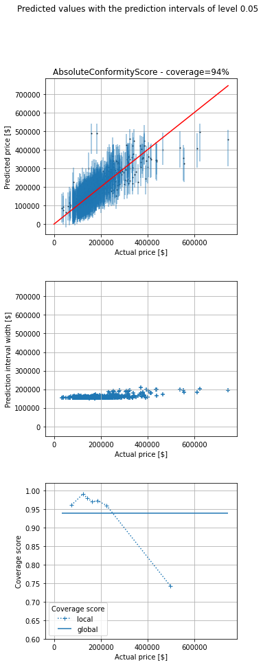
We can see that prediction width is almost the same for all the predictions. The coverage is 94%, close to the chosen value 95%. However, even though the global coverage is (close to) the desired one, if we look at (what I call) the local coverages (coverage for a subset of data points with almost the same price) we can see that coverage is bad for expensive houses (expensive regarding my dataset). Conversely, it is good for cheap ones (cheap regarding my dataset). However, the insights for cheap houses are really poor. For instance, the prediction interval may be [0 ; 180000] for a cheap house, which is not really helpful to make a decision.

Instinctively, I would like to get prediction intervals which width is proportional to the prediction value so that the prediction widths scale to the predictions. This is why I have looked at other non conformity scores, more adapted to my use case.

Conformal predictions with custom non conformity score

Even though I am not a real estate expert, I have some expectations regarding the prediction intervals. As said previously, I would like them to be, kind of, proportional to the predicted value. I would like a small prediction interval when the price is low and I expect a bigger one when the price is high.

Consequently, for this use case I am going to implement two non conformity scores that respect the conditions that a non conformity score must fulfill [7] (3.1 and Appendix C.). I have created two classes from the interface ConformityScore which requires to implement at least two methods get_signed_conformity_scores and get_estimation_distribution. get_signed_conformity_scores computes the non conformity scores from the predictions and the observed values. get_estimation_distribution computes the estimated distribution that is then used to get the prediction interval (after providing a chosen coverage). I decided to name my first non conformity score PoissonConformityScore because it is intuitively linked to the Poisson regression. When considering a Poisson regression, (Y-μ)/√μ has 0 mean and a variance of 1. Similarly, for the TweedieConformityScore class, when considering a Tweedie regression, (Y-μ)/(μ^(p/2)) has 0 mean and a variance of σ² (which is assumed to be the same for all observations). In both classes, sym=False because the non conformity scores are not expected to be symmetrical. Besides, consistency_check=False because I know that the two methods are consistent and fulfill the necessary requirements.

import numpy as np

from mapie._machine_precision import EPSILON
from mapie.conformity_scores import ConformityScore
from mapie._typing import ArrayLike, NDArray

class PoissonConformityScore(ConformityScore):
    """
    Poisson conformity score.

    The signed conformity score = (y - y_pred) / y_pred**(1/2).
    The conformity score is not symmetrical.
    y must be positive
    y_pred must be strictly positive

    This is appropriate when the confidence interval is not symmetrical and
    its range depends on the predicted values.
    """

    def __init__(
        self,
    ) -> None:
        super().__init__(sym=False, consistency_check=False, eps=EPSILON)

    def _check_observed_data(
        self,
        y: ArrayLike,
    ) -> None:
        if not self._all_positive(y):
            raise ValueError(
                f"At least one of the observed target is strictly negative "
                f"which is incompatible with {self.__class__.__name__}. "
                "All values must be positive."
            )

    def _check_predicted_data(
        self,
        y_pred: ArrayLike,
    ) -> None:
        if not self._all_strictly_positive(y_pred):
            raise ValueError(
                f"At least one of the predicted target is negative "
                f"which is incompatible with {self.__class__.__name__}. "
                "All values must be strictly positive."
            )

    @staticmethod
    def _all_positive(
        y: ArrayLike,
    ) -> bool:
        return np.all(np.greater_equal(y, 0))

    @staticmethod
    def _all_strictly_positive(
        y: ArrayLike,
    ) -> bool:
        return np.all(np.greater(y, 0))

    def get_signed_conformity_scores(
        self,
        X: ArrayLike,
        y: ArrayLike,
        y_pred: ArrayLike,
    ) -> NDArray:
        """
        Compute the signed conformity scores from the observed values
        and the predicted ones, from the following formula:
        signed conformity score = (y - y_pred) / y_pred**(1/2)
        """
        self._check_observed_data(y)
        self._check_predicted_data(y_pred)
        return np.divide(np.subtract(y, y_pred), np.power(y_pred, 1 / 2))

    def get_estimation_distribution(
        self, X: ArrayLike, y_pred: ArrayLike, conformity_scores: ArrayLike
    ) -> NDArray:
        """
        Compute samples of the estimation distribution from the predicted
        values and the conformity scores, from the following formula:
        signed conformity score = (y - y_pred) / y_pred**(1/2)
        <=> y = y_pred + y_pred**(1/2) * signed conformity score

        ``conformity_scores`` can be either the conformity scores or
        the quantile of the conformity scores.
        """
        self._check_predicted_data(y_pred)
        return np.add(y_pred, np.multiply(np.power(y_pred, 1 / 2), conformity_scores))

class TweedieConformityScore(ConformityScore):
    """
    Tweedie conformity score.

    The signed conformity score = (y - y_pred) / y_pred**(p/2).
    The conformity score is not symmetrical.
    y must be positive
    y_pred must be strictly positive

    This is appropriate when the confidence interval is not symmetrical and
    its range depends on the predicted values.
    """

    def __init__(self, p) -> None:
        self.p = p
        super().__init__(sym=False, consistency_check=False, eps=EPSILON)

    def _check_observed_data(
        self,
        y: ArrayLike,
    ) -> None:
        if not self._all_positive(y):
            raise ValueError(
                f"At least one of the observed target is strictly negative "
                f"which is incompatible with {self.__class__.__name__}. "
                "All values must be positive."
            )

    def _check_predicted_data(
        self,
        y_pred: ArrayLike,
    ) -> None:
        if not self._all_strictly_positive(y_pred):
            raise ValueError(
                f"At least one of the predicted target is negative "
                f"which is incompatible with {self.__class__.__name__}. "
                "All values must be strictly positive."
            )

    @staticmethod
    def _all_positive(
        y: ArrayLike,
    ) -> bool:
        return np.all(np.greater_equal(y, 0))

    @staticmethod
    def _all_strictly_positive(
        y: ArrayLike,
    ) -> bool:
        return np.all(np.greater(y, 0))

    def get_signed_conformity_scores(
        self,
        X: ArrayLike,
        y: ArrayLike,
        y_pred: ArrayLike,
    ) -> NDArray:
        """
        Compute the signed conformity scores from the observed values
        and the predicted ones, from the following formula:
        signed conformity score = (y - y_pred) / y_pred**(1/2)
        """
        self._check_observed_data(y)
        self._check_predicted_data(y_pred)
        return np.divide(np.subtract(y, y_pred), np.power(y_pred, self.p / 2))

    def get_estimation_distribution(
        self, X: ArrayLike, y_pred: ArrayLike, conformity_scores: ArrayLike
    ) -> NDArray:
        """
        Compute samples of the estimation distribution from the predicted
        values and the conformity scores, from the following formula:
        signed conformity score = (y - y_pred) / y_pred**(1/2)
        <=> y = y_pred + y_pred**(1/2) * signed conformity score

        ``conformity_scores`` can be either the conformity scores or
        the quantile of the conformity scores.
        """
        self._check_predicted_data(y_pred)
        return np.add(
            y_pred, np.multiply(np.power(y_pred, self.p / 2), conformity_scores)
        )

I have then taken the same example as previously. In addition to the default non conformity scores, that I named AbsoluteConformityScore in my plot, I have also considered these two additional non conformity scores.

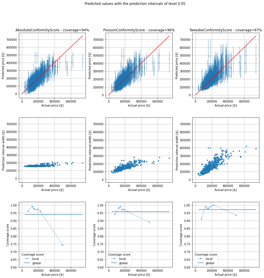
As we can see, the global coverages are all close to the chosen one, 95%. I think the small variations are due to luck during the random split between the training set and test one. However, the prediction interval widths differ significantly from an approach to another, as well as the local coverages. Once again, I am not a real estate expert, but I think the prediction intervals are more realistic for the last non conformity score (3rd column in the figure). For the new two non conformity scores, the prediction intervals are quite narrow (with a good coverage, even if slightly below 95%) for cheap houses and they are quite wide for expensive houses. This is necessary to (almost) reach the chosen coverage (95%). Our new prediction intervals from the TweedieConformityScore non conformity socre have good local coverages over the entire range of prices and are more insightful since prediction intervals are not unnecessarily wide.

Conclusion

Prediction intervals may be useful to make well informed decisions. Conformal prediction is a tool, among others, to build predictions intervals with theoretical coverage guarantee and only a weak assumption (data exchangeability). When considering the commonly used non conformity score, even though the global coverage is the desired one, local coverages may significantly differ from the chosen one, depending on the use case. This is why I finally considered other non conformity scores, adapted to the considered use case. I showed how to implement it in the conformal prediction library MAPIE and the benefits of doing so. An appropriate non conformity score helps to get more insightful prediction intervals (with good local coverages over the range of target values).

References

• Confidence interval – Wikipedia
• Prediction interval – Wikipedia
• Prediction Intervals in Machine Learning
• Conformal prediction – Wikipedia
• OpenML
• GitHub – scikit-learn-contrib/MAPIE: A scikit-learn-compatible module for estimating prediction intervals.

Adapted Prediction Intervals by Means of Conformal Predictions and a Custom Non-Conformity Score was originally published in Towards Data Science on Medium, where people are continuing the conversation by highlighting and responding to this story.