Category: Artificial Intelligence

Deriving the tightest asymptotic bound of a particular tree traversal algorithm

Introduction

Data structures and algorithms are key elements in any software development, especially due to their impact on the final product quality. On the one hand, characterizing a process by means of a widely known and studied algorithm leads to a potential increase in the maintainability of codebases, since there is a large volume of open source resources and documentation available on the web. But, the main feature that is the reason why much effort is spent when deciding which data structure to use for the representation of information or the ideal algorithm for the performance of a given task is efficiency, both in terms of memory and time. In short, the choice of a good procedure or structure usually produces an advantage over other products on the market, whose response time, computational resources needed to fulfill its purpose or scalability are inadequate for its requirements.

Therefore, in order to make proper decisions in this regard, it is necessary to measure the cost of the algorithms accurately to subsequently perform studies in which a sufficiently valid comparison can be established to discard implementations or data structures that do not fit the product requirements, which often involve time and space constraints. As such, these two quantities are quantified by their asymptotic growth as the size of the input data provided grows to infinity. That is, the measure of how efficient an algorithm is depends on the growth of the time or space resources required for its execution given a certain increase in the input size, whereby the more they increase with the same variation of the input size, the worse its performance is considered, since they will need more resources than necessary. On the other hand, the selection of a suitable data structure on which efficient algorithms can be applied depends mainly on the complexity of the information to be modeled, although the final objective is that the algorithms determined by their operations (add(), remove(), search(element)…) have the minimum asymptotic growth achievable.

Objective

In this work, with the aim of showing the method to describe the time complexity of an algorithm and to allow its comparison with other alternatives, we will first start with a data structure, namely a perfectly balanced binary tree, and an algorithm executed on it. Subsequently, the format of its input will be formalized, visualizations will be built to understand its composition, as well as the procedure trace, and finally the ultimate bound will be reached through a formal development, which will be simplified and detailed as much as possible.

Algorithm Definition

The algorithm we are about to work with involves a binary tree with the restriction of being perfectly balanced. By definition, a binary tree is a pair formed by a set of nodes and another set of edges that represent connections between nodes, so that each of the nodes of the set has a connection with exactly two nodes known as child nodes. And, of all the existing trees that can be formed from this definition, here we are only interested in those designated as perfect.

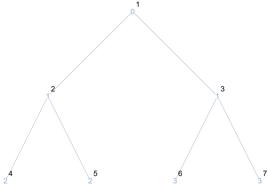
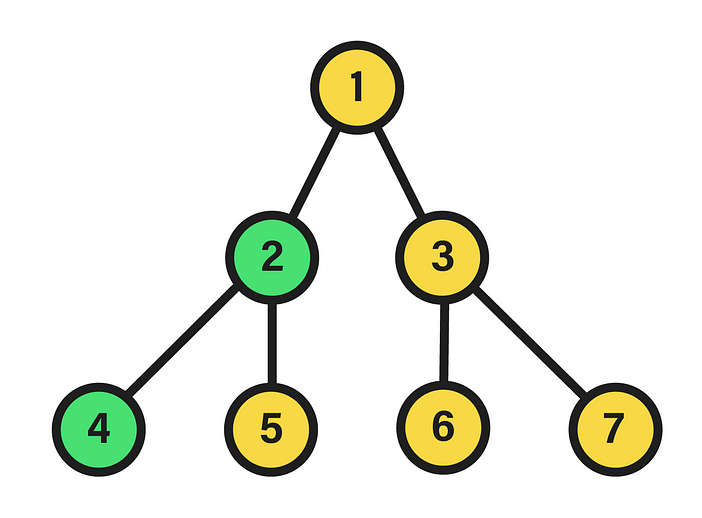
A perfect binary tree is distinguished by the equality in the depth of its leaf nodes, i.e. those of its last level, and by the constant number of children equal to two in the remaining nodes. The depth of a node within the tree, in turn, is the length of the path between its root and the node in question. Hence, the appearance of the data structure will be akin to:

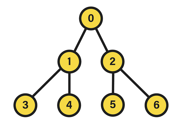
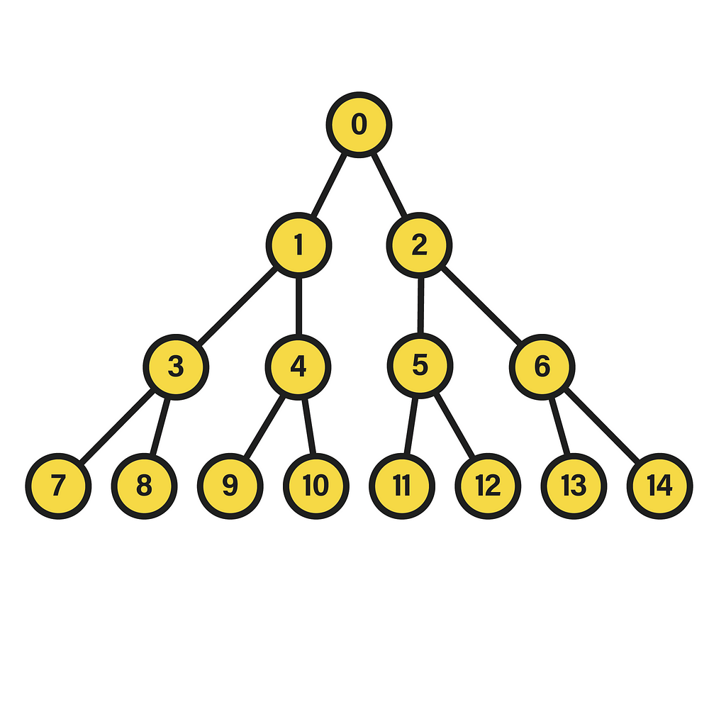
In this particular case, we are dealing with a perfect binary tree of depth two, since the nodes of the last level fulfill the condition of having the same depth, equivalent to that value. Additionally, in the picture the nodes have been numbered in a certain way that will be useful in this context. Specifically, the integer corresponding to each node stems from the execution of a breadth-first traversal starting from the root, which is equivalent to a level-order traversal given the tree hierarchy. Therein, if the visited nodes are numbered starting from 0, a labeling like the one shown above will be settled, in which each level contains all the nodes assigned to integers between 2^l-1 and 2^(l+1)-2, where l is the level. To see the source of this expression, it suffices to find a function that, with a level l as input, returns the minimum integer in the interval of that level, as well as another function that calculates the opposite, i.e. the maximum.

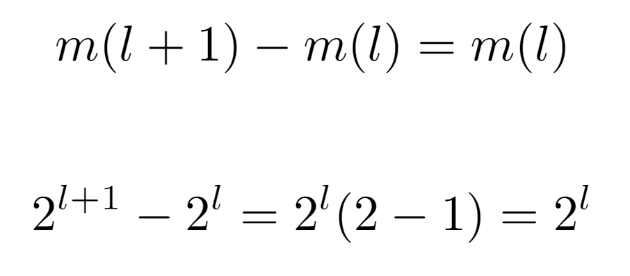
First, let m(l) be the function that returns the minimum. Thus, by observing the sequence it should follow as the input increases, we notice the pattern {0,1,3,7,15,31,63…}. And, when searching for its initial values in OEIS, it yields a match with the sequence A000225. According to the definition of this sequence, its values are given by the expression 2^l — 1, but, to see why this is the one that models the progression of m(l), it is necessary to establish a relation between two contiguous evaluations m(l) and m(l+1), which will lead to such formulation. Then, if we consider the minimum value for one level l and that of the next, we can start from the assumption that the difference between the two is always equal to the number of nodes existing in the level with the least number of nodes. For instance, in level 1 there are only two nodes, whose labels are {1,2}. The minimum value in this level is 1, and the next one is 3, so it is easy to verify that 3=1+2, that is, the minimum value of level {1,2} plus the number of nodes in it. With this, and knowing that the number of nodes in a level, being a binary tree, is exactly 2^l nodes, we arrive at the following formulation of m(l):

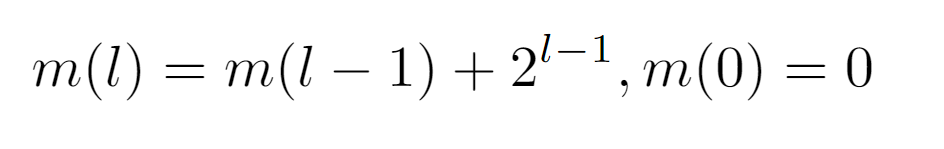
In summary, m(l) is expressed as the minimum integer in the previous level m(l-1) plus the nodes contained in it 2^(l-1), in addition to the base case m(0)=0.

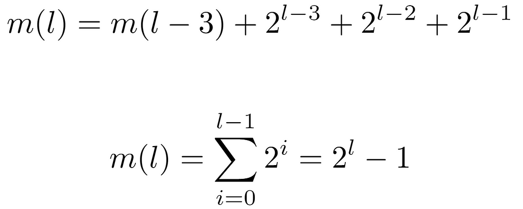
So, when expanding m(l) by evaluating its recursive term, a pattern appears with which this function can be characterized. Briefly, every power of 2 from 0 arising from m(l-l) up to l-1 is aggregated. Finally, after solving the summation, we arrive at the same expression present in the definition of A000225. Consequently, we now proceed to obtain the maximum integer at level l, which is denoted by a new function M(l). In this case, the sequence formed by its evaluations is of the form {0,2,6,14,30,62…}, also recorded in OEIS as A000918. For its derivation, we can leverage the outcome of m(l), so that by knowing the number of nodes present at each level, M(l) can be defined as the minimum integer at each level m(l) plus the number of nodes in it.

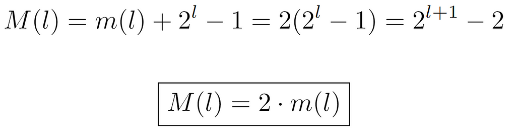
In order to arrive at the ultimate expression 2^(l+1)-2, we add m(l) and the number of nodes at that level except for one, the minimum. And, as this value coincides with m(l), we can conclude M(l)=2m(l).

After defining the data structure the algorithm will work with and discovering some potentially useful properties for a complexity analysis, the algorithm in question, expressed in pseudocode, is introduced:

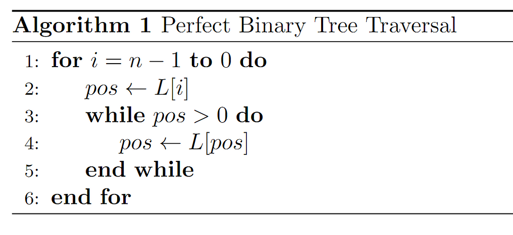
At first, although we will later expand on this in detail, the input consists of a vector (array) denoted as L where the binary tree is represented. With it, every entry of the array corresponding to nodes in the tree is linearly traversed by means of a for loop. And, within each iteration of this loop, a temporary variable pos is initialized to store array elements, so it will have the same type (integer). In addition, in the iteration, all the nodes that form the path from the root of the tree to the node represented by the array entry on which the for is running are traversed via the while loop nested within it. For this purpose, the exit condition pos>0 is set, which corresponds to the situation where pos has reached the root. As long as this condition is not met, pos will update its value to that of its parent node, so assuming that the input structure is correct, there is a guarantee that for every node in the tree the while loop will always reach the root, and therefore terminate.

Input Characterization

To grasp this process, it is essential to be familiar with the input format. In particular, the way in which the binary tree can be represented in the form of an array, being the structure used by the algorithm. To this end, and to simplify this representation, a transformation is performed in the labeling of the tree nodes, so that the breadth traversal they were labeled with at the beginning is executed from the root node starting at the integer 1. Or, seen in another way, 1 is added to the original label of all nodes.

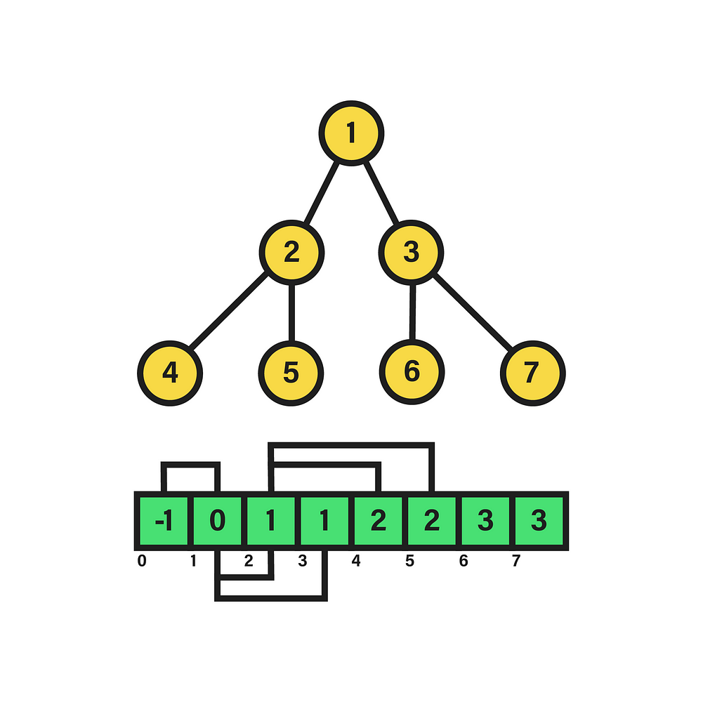
The result of the aforementioned transformation is shown above. As evidenced, the minimum and maximum values of the labels at each level have also been modified. Although, due to the properties of the transformation, it is sufficient to apply its inverse to the functions m(l) and M(l) to re-characterize the label sequences correctly.

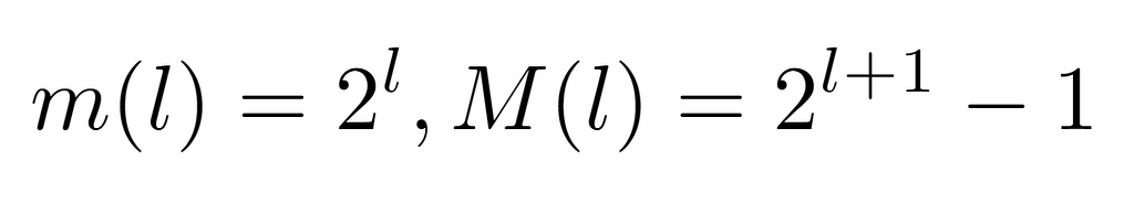
Consequently, if the transformation on the nodes consists of adding 1 to its label, its inverse subtracts such quantity. This way, after applying the inverse transformation to both functions, we arrive at the upper expressions, modeling the sequence of minimum and maximum value labels for each tree level. On the other hand, by means of the new labeling, the data structure can be represented as an array, like the one our algorithm takes as input. Similarly, since it is a perfect tree, we know that it will have a regular structure in terms of number of nodes, as well as their location in the hierarchy. Because of this, considering the input array L[n+1], we can relate its indexes to the values stored in those positions.

For example, as depicted in the above image next to the “linked” representation of the tree, we can map the labels of each node to the array indexes, so that L[1] stands for the instance of the root node, L[2] and L[3] for their respective child nodes, and so on up to the terminal nodes. However, it is also necessary to denote their edges explicitly, so it is decided to store in the array values the label corresponding to the parent node of a given one by a certain index. In short, for each node i (index) of the array, the value stored in L[i] corresponds to the label of i’s parent node. Yet, as a matter of correctness, the first index of the list L[0] is not considered to correspond to any node. Moreover, its value is set to -1 to denote that it has no node above it in the hierarchy.

In view of this idea, it is worthwhile to study the properties of the sequence {-1,0,1,1,1,2,2…} (A123108), or even to find a function to span its values, which will be valuable in the analysis. Hence, it is first important to consider how the child nodes and the parent L[i] of a given node i are determined.

Regarding the child nodes of a given node i, if we account that any subtree of the original structure is also a perfect tree, it can be inferred that m(l) will serve its purpose within the scope of the subtree, resulting in the difference between the labels of any node and its left child being i (below instead of i is denoted as 2^l, both equivalent), which coincides with the amount of nodes at the lower level.

Furthermore, to view that it is fulfilled in all subtrees, offsets α and β are attached to the left child and parent node labels repectively, resulting in the equivalence 2α=β.

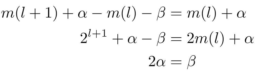
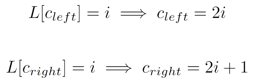
Assuming that the offsets do not exceed the node limit at their level, the amount of nodes present at the level of the child node located between its minimum m(l+1) and itself is twice that of the same magnitude considered at the upper level with its parent node. Hence, by doubling the number of nodes at each level by definition of a perfect binary tree, it is concluded that the label of the left child node of one i is given by the expression 2i, being that of its right child 2i+1 accordingly. Likewise, a node i will always have a parent node, except in the case where it is the root, whose parent will be L[0], which is not treated as a tree node.

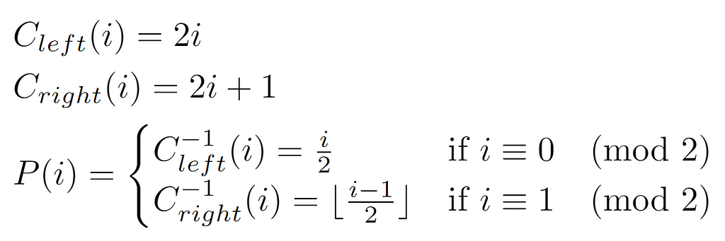
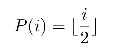
To determine the function that outputs the label of the parent node, we first define the functions Cleft(i) and Cright(i) that get the respective child nodes. In this manner, if these functions transform the label in such a way that the result is equivalent to a descent in the hierarchy, their inverses will lead to the opposite effect, which is expected in case we want to retrieve the parent. After defining P(i) as the function that returns the parent node of i, equivalently denoted as the value in the vector L[i], it is necessary to make a distinction in the expression applied for its computation according to the properties of the input. That is, if the node is labeled even, that means it is the left child of some node, so the inverse of Cleft(i) will be invoked. On the other hand, in case it is odd, the function P(i) has as expression the inverse transformation to Cright(i).

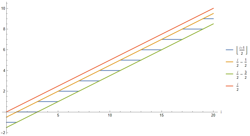
Graphically, both formulations for even and odd labeled nodes exhibit asymptotically similar growth as i increases. Even, due to the properties of the floor function it is possible to constrain the values of P(i) with odd i via i/2-dependent bounds and a constant. As a result, this leads to the following property:

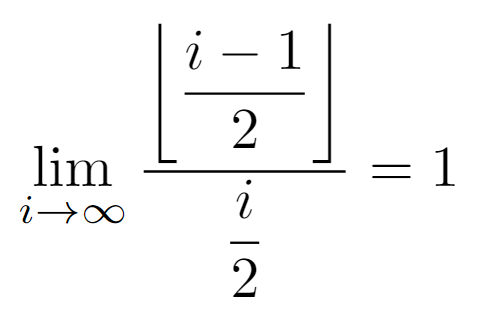
By observing the above graph it is not possible to guarantee that the asymptotic growth of both subexpressions of P(i) is exactly equal. But, after deriving the bounds for the odd case and determining that the dependence has order O(i), we can compute the limit when the node label tends to infinity of the ratio between the two functions, being their growths equivalent as expected.

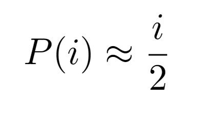
Consequently, for simplicity it would be convenient to provide a single formulation for P(i) regardless of the input received, so the simplest option is to consider the growth order of the even case i/2, since the remaining case has the same asymptotic growth.

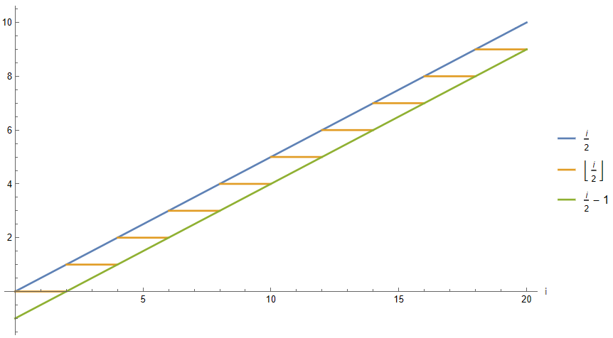
Nevertheless, the i/2 operation does not return integers for nodes with odd label, so to address this concern it is decided to apply the floor function again to i/2. Visually, the value of Floor[i/2] can be bounded in a similar way by the original function and its same value minus 1 due to the properties of the floor function. But, as the objective is to reach a correct expression for P(i), not an approximate one that serves for an asymptotic analysis, still, it is deemed necessary to define it from the floor of i/2.

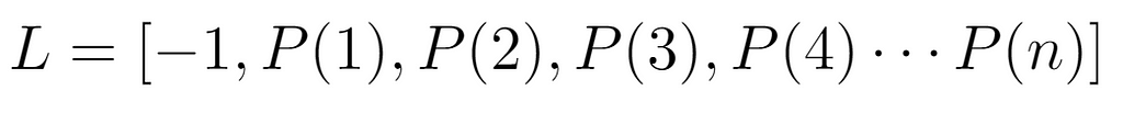
The main reason for selecting such definition arises from the formal definition of the input array:

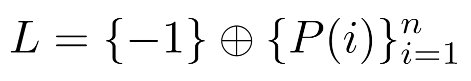
Since L contains the labels of the parent nodes determined by each array index, it is possible to characterize them from the function P(i), where i in this case is a valid index. In other words, the first value L[0] must equal -1, which is denoted in a special way without the use of P(i) as it cannot generate that value. Then, the base array {-1} is concatenated with the sequence {P(1),P(2),P(3)…} whose length is the total number of nodes and whose values correspond to the parent nodes of the label sequence {1,2,3…}.

GenerateTree[n_] := Flatten[{-1, Table[i/2, {i, 1, n}]}]
GenerateTree[15]

Once the sequence contained in the input array has been modeled, above is the Wolfram code needed to generate a tree with 15 nodes, resulting in L={-1, 1/2, 1, 3/2, 2, 5/2, 3, 7/2, 4, 9/2, 5, 11/2, 6, 13/2, 7, 15/2}. As expected, by not using the Floor function in P(i), nodes with odd index return rational numbers, so after redefining the GenerateTree[] function with the appropriate P(i), the correct sequence L={-1, 0, 1, 1, 1, 2, 2, 2, 2, 3, 3, 3, 4, 4, 4, 5, 5, 5, 6, 6, 6, 7, 7} is achieved:

GenerateTree[n_] := Flatten[{-1, Table[i/2 // Floor, {i, 1, n}]}]
GenerateTree[15]

Input Visualization

Besides building the array, it is appropriate to visualize it to ensure that the indexes and values contained in it match its definition. For this purpose, Wolfram’s graphical features are used to automate the tree visualization process from the sequence created by GenerateTree[]:

PlotBinaryTreeFromList[treeList_List] := 
 Module[{n = Length[treeList], edges},
  edges = Flatten[Table[{i -> 2 i, i -> 2 i + 1}, {i, 1, Floor[n/2]}]];
  edges = Select[edges, #[[2]] <= n &];
  TreePlot[edges, VertexLabeling -> True, 
   VertexRenderingFunction -> ({Inset[treeList[[#2]], #1]} &), 
   DirectedEdges -> False, ImageSize -> Full]]
n = 31;
treeList = GenerateTree[n]
PlotBinaryTreeFromList[Drop[treeList, 1]]

When building a tree with exactly 31 nodes, L={-1, 0, 1, 1, 1, 1, 2, 2, 2, 3, 3 … 14, 14, 15, 15}, which graphically resembles the following:

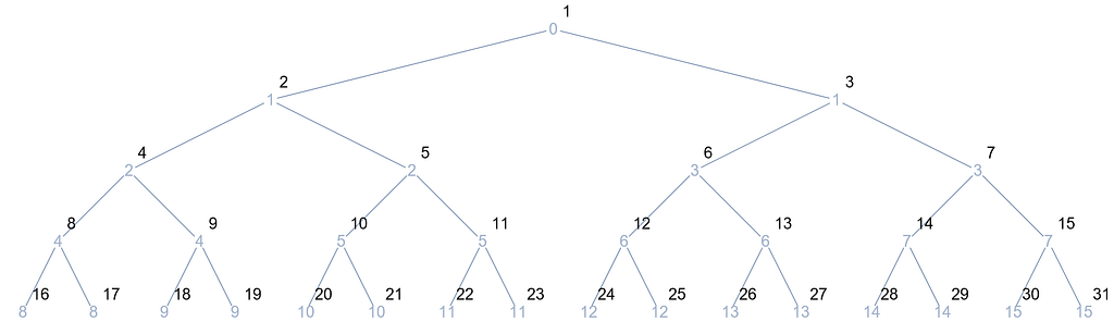
Concretely, the blue text denotes the index of the parent node, while the other text in black illustrates the label of the node in question.

Implementation

Now with a well-defined input, it is possible to comprehend at a more abstract level what the operations of the tree traversal actually do. On one side, the outer For[] loop traverses through all the nodes in level order from the lowest level to the one where the root is located. And, for each node the While[] loop traverses the path from the root to the visited node in reverse order, although the important aspect for the time complexity bound is its length.

TreeIteration[v_List] := Module[{n, pos}, n = Length[v];
  For[i = n, i >= 0, i--,
   pos = v[[i]];
   Print["FOR: ", i];
   While[pos > 0,
    Print["While: ", pos];
    pos = v[[pos + 1]];
    ]]]

So, after implementing it in Wolfram, some Print[] are included to display the index of the parent node of the nodes it traverses during its execution, enabling an easier reconstruction of its trace.

Output

n = 7;
treeList = GenerateTree[n]
TreeIteration[treeList]
PlotBinaryTreeFromList[Drop[treeList, 1]]

Running the algorithm with a 7-node tree, represented as L={-1, 0, 1, 1, 1, 1, 2, 2, 2, 3, 3}, yields the following outcome:

FOR: 8
While: 3
While: 1
FOR: 7
While: 3
While: 1
FOR: 6
While: 2
While: 1
FOR: 5
While: 2
While: 1
FOR: 4
While: 1
FOR: 3
While: 1
FOR: 2
FOR: 1
FOR: 0

At first glance, the trace is not too revealing, so it should be combined with the tree depiction:

In the first iteration of the for loop, the traversal starts at the last node of the lowest level, whose parent has index 3. Subsequently, this node is also visited by the while loop, until in the next iteration it reaches the root and ends. In the succeeding for iteration, the same process is performed with the difference that it begins with the node with index 6, whose parent node is the same as before. Thus, it can be noted that the for is actually traversing all the existing paths in the tree that connect each of the nodes to the root.

Analysis

With the algorithm in place, and after having fully characterized its input and understood its operation, it is suitable to proceed with its analysis, both in terms of memory and time. On the one hand, the analysis of the memory occupied is straightforward in this case, since the algorithm does not need additional memory to perform its task, beyond the integer value pos in which the node traversed in each iteration is stored. Accordingly, the asymptotic bound representing the additional memory consumption is constant O(1). And, if we consider the space occupied by the input, an amount of memory of order O(n) would be required, where n is the number of nodes in the tree, or more precisely O(2^d), where d is the tree depth.

On the other hand, to determine the time complexity bound, we must define an elementary operation to be accounted for. For this algorithm, it is established as the asingnation executed inside the while loop, which at an abstract level can be considered as the traversal of an edge between a node and its parent. Therefore, to ascertain how many times this operation is invoked, the cost of the algorithm is first decomposed into two functions. There is, on one side, the cost Tf(n) of the for loop, which represents the total of one algorithm’s execution. This, in turn, is defined as the sum of the costs incurred by the while loop, designated as Tw(i).

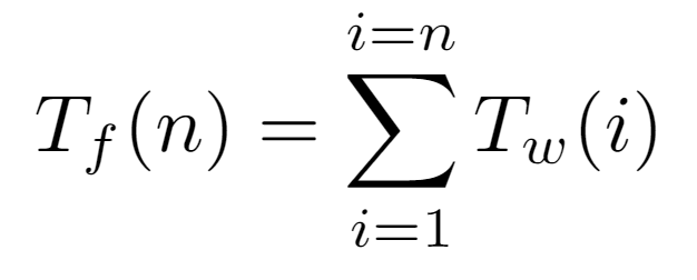
For all nodes i contained in the array, we need to determine how many elementary operations are involved in the traversal of the path from the root to i, so we append the corresponding Tw(i) evaluation. Specifically, that function will return the exact number of assignments caused by a certain input node. Thus, since we know that the first L[0] cannot walk any path to the root, it is not counted, keeping the sum limits between 1 and the number of nodes n in the tree.

Before continuing, we proceed to demonstrate that the application of the function P(i) to a node i located at level l of the tree results in the label of a node located at the immediately upper level, since the elementary operation considered in this analysis is equivalent to pos=P(pos), mainly due to the input features:

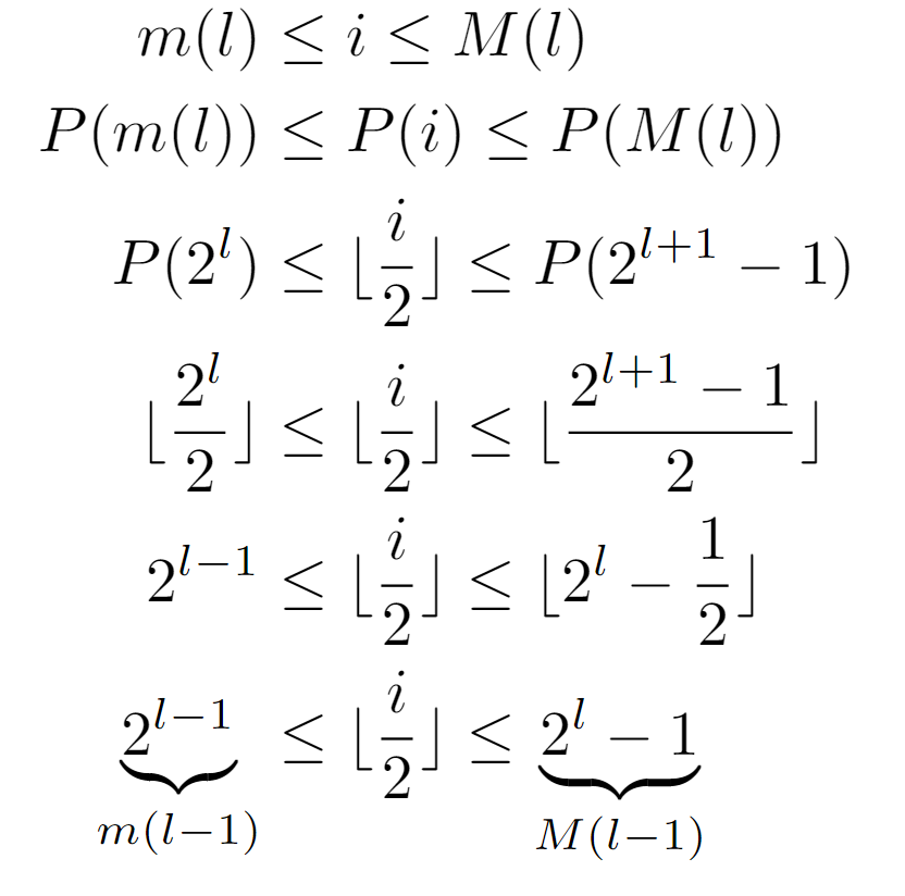
As shown, we begin with the inequality that any node must fulfill with respect to the level at which it is found, being its label bounded by the functions m(l) and M(l), and assuming that l is its level. Afterwards, when applying P, several simplifications can be effected, leading to the conclusion that P(i) lies between 2^(l-1) and 2^l-1, both coinciding with the evaluations m(l-1) and M(l-1), suggesting that after the transformation the resulting node is located at level l-1. With this, we are demonstrating that after several iterations of the while loop, the node stored in pos will have a level closer to the tree root. Consequently, if enough of them are completed, the path is guaranteed to reach the root and terminate. Although, in case of considering an infinite tree this might not hold.

Approach 1

At the moment, we know that the complexity is driven by Tf(n), despite the lack of an exact expression for Tw(i), so we proceed to discuss three different ways to characterize this function, and thereby the overall asymptotic growth of the execution time.

Regardless of how the remaining function is found, a constraint on the tree nodes will be met in all analyses. Namely, since they all have a single parent, except the root, we can ensure that the path length between an arbitrary node located at a level l and the root is equal to l. Primarily this is due to the property demonstrated above, although it can also be evidenced by the realization that each node present on such a path is at a different level, which can vary from 0 to l. Then, as the while loop traverses every node in the path, it is concluded that the operations counted in Tw(i) are exactly l.

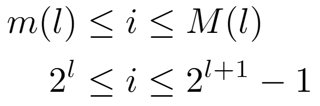
Now, the analysis is focused on computing the level of a given node, so we start from the upper inequality. That is, the label of a node i is at a level l bounded by m(l) and M(l), yielding two conditions with which the level can be accurately quantified:

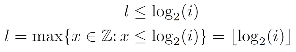
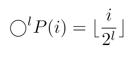
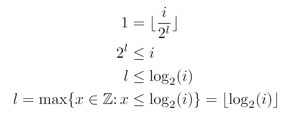
On the one hand, solving from the left side of the inequality leads to a condition reducible to a floor operation on log_2(i), by its own definition. From this, it can be inferred that the level is equal to that quantity, although the other condition of the original inequality still needs to be verified.

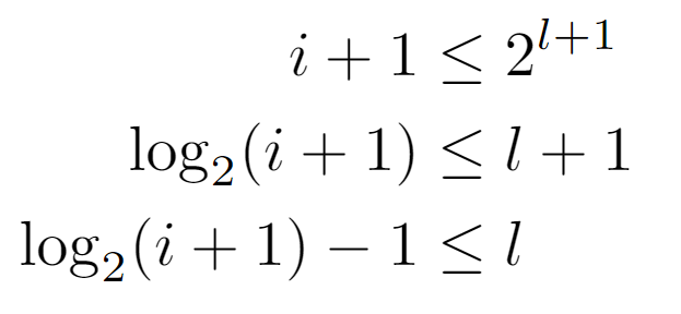
Starting from the right-hand side, we arrive at a lower bound for l, which a priori appears to be complementary to the preceding. However, after operating and applying the definition of the ceiling function, we arrive at the following formulation for the level, since its value is the minimum integer that satisfies the last inequality shown above.

Recapitulating, so far we have derived several expressions for the level of a node i, which at first could be thought of as bounds of that value due to their nature. Nonetheless, the level must be an integer, so it is conceivable to check the distance between them, just in case it were small enough to uniquely identify a single value.

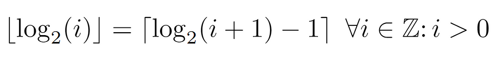
In summary, it is proven that both expressions are identical for all the values that the node labels may have. Therefore, the level of a node can be inferred by either of the above formulae, the left one being the simplest, and so the one that will be used in the analysis.

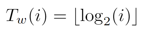
As the level of i coincides with the elementary operations of the while loop, the cost Tw(i) is defined analogously to the node’s level from which the path to the top must commence.

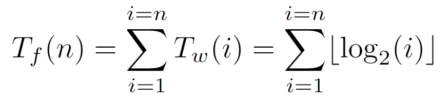
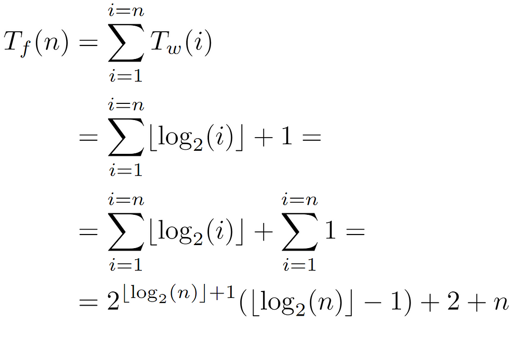
Next, with an expression for the cost of each iteration of the for loop as a function of the initial node, we can try to find the sum of all the costs generated by the nodes of the tree. But, as there is a floor function in each summand, we will first study the impact of not applying this function on the ultimate bound, in order to simplify the summation, as well as the resulting bound in case the floor becomes dispensable.

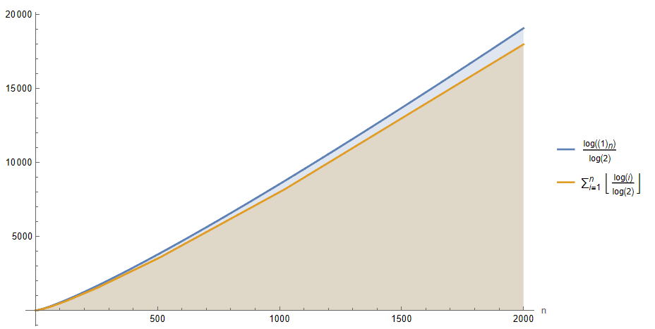
If we plot Tf(n) for a decent range of n, a slight difference is discernible between the function with the floor of each summand removed and the original one. Particularly, the one that directly sums the logarithm values without any additional transformation appears to be a upper bound of the actual complexity, so if we proceed to solve the sum where each term is directly log_2(i), we can arrive at a bound that asymptotically may be somewhat larger than the actual one, establishing itself as the upper one:

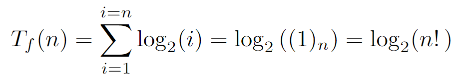
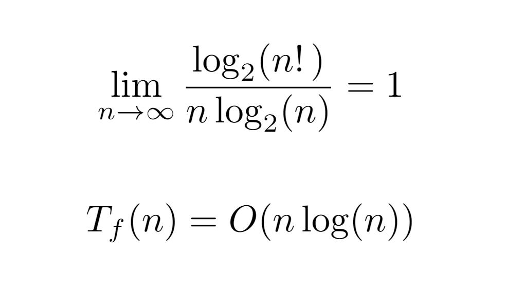
By expressing the sum in a closed form, we could assume that the algorithm requires an execution time no greater than the order O(log(n!)) with respect to the number of nodes in the input tree. Still, this bound can be further simplified. For instance, if we consider that in each iteration of the for loop, which is executed as many times as n nodes, a work is performed proportional and not higher than the maximum level of the tree, we would get an upper bound of order O(n log(n)). As a consequence, if we compare it with the previous order O(log(n!)) through the limit of its ratio when the input tends to infinity, we conclude that both are equivalent, allowing the simplification of the upper bound of the algorithm’s runtime to O(n log(n)).

At this juncture, the upper bound ensures that the runtime overhead of the algorithm does not exceed the order O(n log(n)) in terms of growth with respect to the input. However, the interest of the analysis resides in bounding the cost as much as possible, i.e., finding the tight bound, not an upper one, which in some cases may differ significantly. For this, it is necessary to find a closed form for the sum Tf(n) above, especially when the floor function is applied to the summands. Intuitively, the application of the floor will reduce the value of each term to some extent, and the ultimate value may vary due to the dependence between the upper limit and the size of the tree.

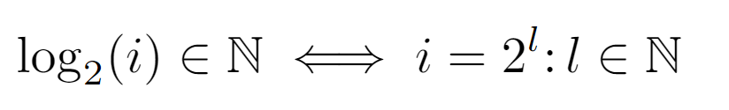
Firstly, for log_2(i) to be an integer and to avoid applying the floor transformation, the node label must be of the form 2^l, where l must necessarily refer to the level at which it is encountered.

Coincident with m(l), above it is shown that all nodes i=m(l) whose label is the minimum of their level will result in log_2(i) being an integer, namely l.

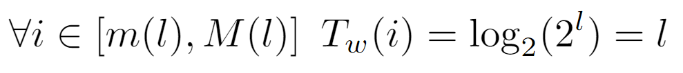
Therefore, by feeding all labels between m(l) and M(l) as input to the floor(log_2(i)) function, it should yield its level, which has been found to coincide with that of the “representative” m(l) node of that level. Briefly, this allows to assume that every node of a particular level will incur in the same cost Tw(i), as the path’s length from any one of them to the root is exactly equal to l.

Subsequently, the number of nodes at each level is deduced, which as one might guess without this step is 2^l, that is, if at each level the number of nodes of the previous one is doubled, for a certain level this quantity will be given by the product of the branching factor by itself l times.

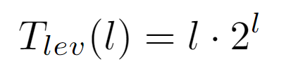
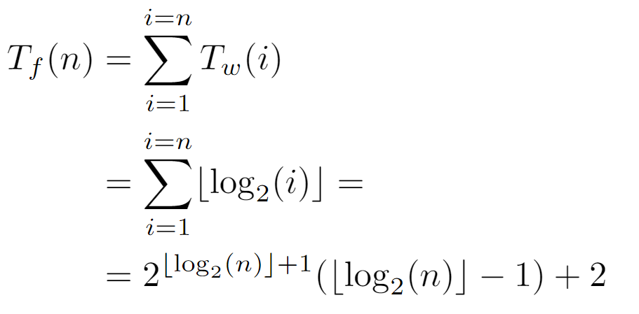
In conclusion, the runtime cost of the algorithm at all nodes of the same level l is the product between the length of the path to the root, coincident with the level, and the number of nodes in it. And, from this result a closed form for Tf(n) dependent on the depth d of the tree can be drawn:

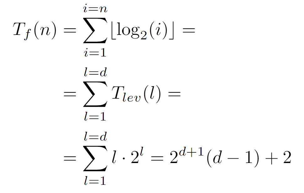
By rewriting the sum as a function of the levels from 0 to the depth, we arrive at the above expression, which can be concretized by defining the relationship between d and the total number of nodes n:

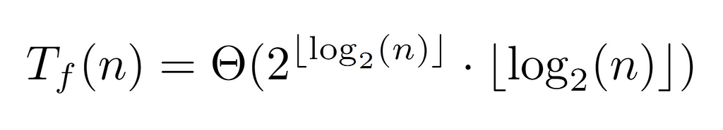
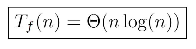
Since n is the label of the last node, floor(log_2(n)) guarantees to return the value of the last level, which in turn coincides with the depth d. Thus, by the above formulation of the complete cost Tf(n) we conclude with the following tight bound:

At this point, it is worth trying to simplify it, so that it is featured by a simpler expression. For this reason, we proceed to calculate its ratio with the previous upper bounds, which will mainly show the difference between both in case they are asymptotically equivalent, or diverge in the opposite case (although it could also converge to 0).

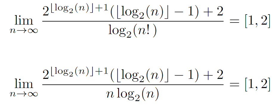
Nevertheless, the limits of the ratio produce the same result for both upper bounds, being asymptotically equivalent. And, as they lie on a real interval, it can be inferred that the tight bound is equivalent to the upper one, at least asymptotically, since the ratio indicates a negligible difference at infinity.

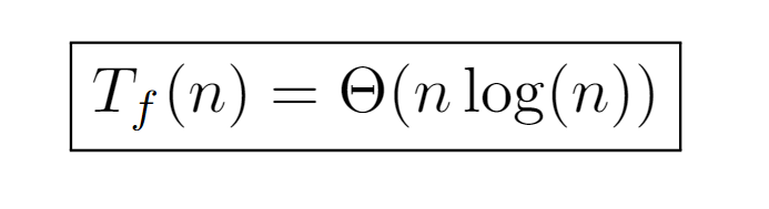
Finally, the time complexity of the algorithm is determined by the top order, which can be achieved in several ways as we will see below. Before continuing, though, it is worth noting the relationship between the two expressions found for the tight bound. While the latter depends directly on the number of nodes, the original one can be formed by rewriting the one shown above replacing n by the number of nodes at the last level, which contributes to a better understanding of the dependence between the runtime and the properties of the data structure involved.

Approach 2

Another way to proceed with the analysis is by defining each value contained in the input array:

Each one is identified by a concrete evaluation P(i), from which the following constraint can be inferred:

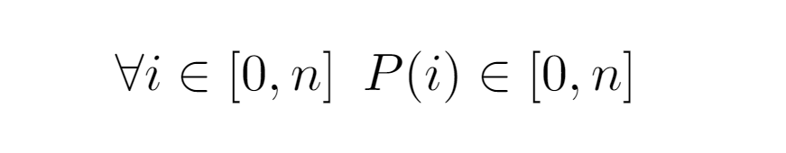
By representing P(i) an ascent in the tree, any input bounded by [0,n] that can be provided to the function will always return a result present in the same interval, which leads to the formalization of the traversal performed by the while loop and whereby we will achieve Tw(i):

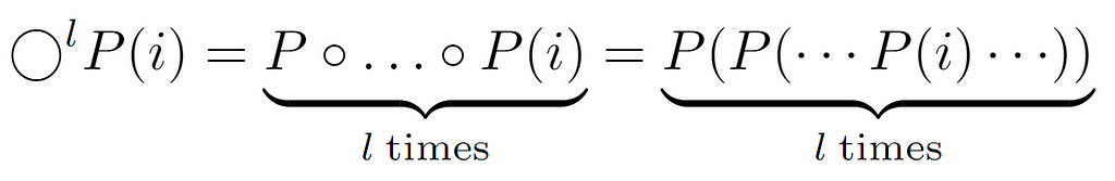
At the beginning of the traversal, any node i is chosen, ascending to its parent P(i), then to its ancestor P(P(i)) and so on until reaching the root with label 1. Actually, the loop stops when reaching the “node” L[0], however, here it is considered that it stops at the root, since the difference in cost will be constant. So, above we formalize this process by composing P(i) a variable number of times, which as we know coincides with the length of the path to the root, can be set equal to the node’s level l.

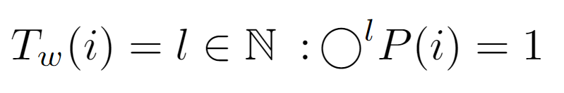
With this approach, the cost Tw(i) is defined as the level of the input node, which can also be acquired by finding the integer that satisfies the upper equality.

At this point, when obtaining the integer l that causes the repeated composition to result in 1, we first apply the properties of the floor function to describe the composition in a closed form. Also, it is demonstrable that the composition of the function P results in the above expression.

Thereafter, by definition of the floor function, an inequality is established between the closed form of the composition and the outcome it should reach. That is, the equality dictates that after l compositions exactly the value of the root is reached, although, since the argument of the floor may be greater than 1, we proceed from the inferred inequality. Finally, we conclude with an expression for the level of a certain node i, which we will use to find Tf(n), and hence the complexity.

When replacing Tw(i) by the level of node i, the summation produced is equivalent to the one solved in the previous analysis, so the final expression is also equivalent.

Ultimately, the tight bound derived from this procedure is of order nlog(n), coinciding with the previously inferred one. In turn, it may also be rewritten as a function of tree’s depth, which in certain situations becomes helpful.

Approach 3

Lastly, we will explore an alternate way to perform this analysis and acquire the prior asymptotic bound. In this case, we shall start from the label i of a parent node stored in the array. This label at low level is represented as a positive integer, specifically in base 2. Therefore, its binary form can be denoted as follows:

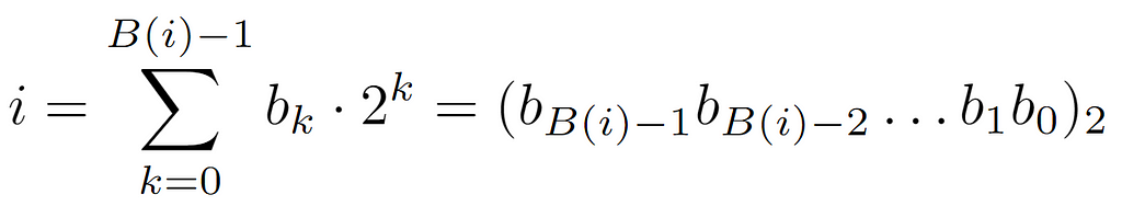
On one hand, it is defined as the sum of the products of the bits by their value in the corresponding base, which in a compact format is formalized as a group of bits whose subscript denotes such value.

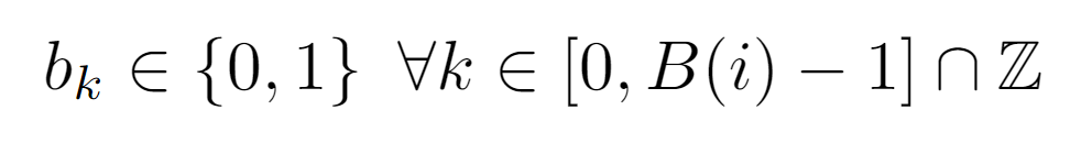
Each of the bits is an integer 0 or 1, whose subscript belongs to the interval of the integers comprised between 0 and B(i)-1, where B(i) is the function that returns the length of the binary representation of the integer i.

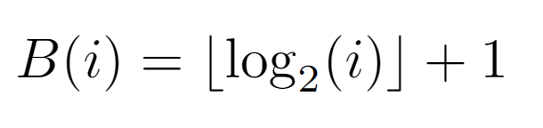
As for its formulation, it remains proven that the number of bits needed to describe an integer in base 2 is given by the above equality. A priori, the logarithmic term is identical to the expression describing the level at which node i is located, so we can begin to elucidate the rest of the procedure.

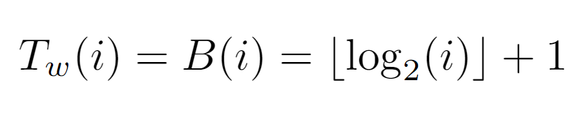
To calculate Tw(i), it is necessary to account for the effect of P(i) on the binary representation of the node label. Simply put, the label resulting from the repeated application of P(i) must be 1, or in this case for simplicity 0. Therefore, by dividing the label by 2 and applying the floor function, it can be guaranteed that in binary the equivalent of this function is a shift operation to the right. So, after B(i) shifts, the resulting label will be 0, concluding the path of the while loop and incurring a cost proportional to floor(log_2(i))+1.

Likewise, when substituting B(i) in the sum of the overall cost, in this analysis we end up with an additional term n, which, being smaller than the final value, is asymptotically negligible.

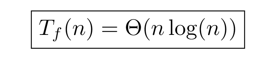
In conclusion, with this procedure the same tight bound is deduced, keeping the runtime cost of the algorithm classified by the order nlog(n).

Time Measurements

Finally, after the theoretical analysis, experimental measurements will be collected of the time it takes to finish the algorithm for inputs of different sizes, in order to show how well or poorly the runtime growth matches the tight bound.

data = Flatten[
   ParallelTable[
    Table[{n, 
      AbsoluteTiming[TreeIteration[GenerateTree[n]]][[1]]}, {index, 0,
       n}], {n, 1, 300}], 1];

To this end, several Wolfram functions are used in the measurement process. The most significant of these is AbsoluteTiming[], which records the time in seconds it took to run the algorithm with a tree consisting of n nodes. Here, we do not select values of n that are powers of 2, we simply consider that the input is a complete tree instead of a perfect one in order to observe how the execution time grows in relation to the number of nodes. Then, measurements are taken for n from 1 to 300, performing n runs for each corresponding number of nodes.

nonlinearModel = NonlinearModelFit[points, a*x*Log[x], {a}, x]
ListPlot[{points, Table[{x, nonlinearModel[x]}, {x, 0, 300}]}, 
 PlotStyle -> {Red, Green}, ImageSize -> Large, 
 AxesLabel -> {"n", "Time (s)"}]

Afterwards, a fitting model of the form c*nlog(n) is defined in which c represents a constant used as a parameter, adjusting its value to the measurement dataset as dictated by the NonLinearModelFit[] function.

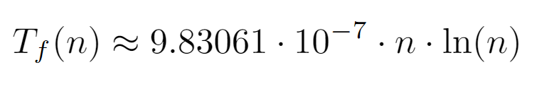
Once the model has been fitted, the top outcome is generated, the interpretation of which is significantly more meaningful when plotted against the data points:

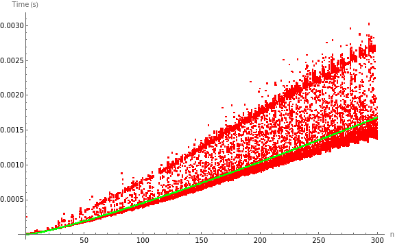
As seen, the dataset shows some variability due to practical interferences in the measurement process. However, the growth as n is increased is clearly similar to an order nlog(n), which is also remarkable in comparison with the location of the model, being situated in a zone somewhat lower than the average between the two regions that visibly show a higher density of measurements.

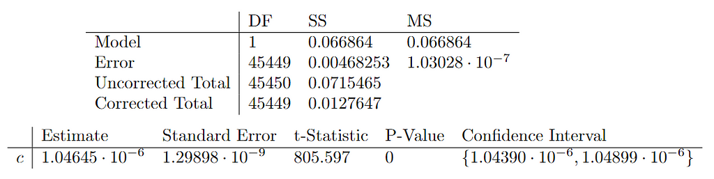
Finally, with the previous fitting results and an adjusted R² of 0.934551, it can be concluded that the model correctly captures the growth trend of the dataset. Though, its variability translates into a slight uncertainty in the value of the c constant.

Conclusion

The formal analysis of the algorithm characterizes the asymptotic growth of its execution time by the order Θ(nlog(n)). Such bound has been calculated from three different approaches, although all of them are based on the same idea of determining the depth of each tree node. In the first one, the level was used as the depth measure, which is equivalent to the number of times P(i) must compose with itself to reach the label of the root node, and, in turn, to the number of bits needed to represent the label of the initial node i in binary.

Also, as a final note, it is worth mentioning that most of the Wolfram code involved in this analysis was generated by the GPT-4o model from ChatGPT.

---

Time Complexity Analysis of Perfect Binary Tree Traversal was originally published in Towards Data Science on Medium, where people are continuing the conversation by highlighting and responding to this story.

Unpacking the six core traits of AI agents and why foundations matter more than buzzwords

The tech world is obsessed with AI agents. From sales agents to autonomous systems, companies like Salesforce and Hubspot claim to offer game changing AI agents. Yet, I have yet to see a compelling truly agentic experience built from LLMs. The market is full of botshit, and if the best Salesforce can do is say their new agent performs better than a publishing house’s previous chatbot, that’s disappointingly unimpressive.

And here’s the most important question no one is asking: even if we could build fully autonomous AI agents, how often would they be the best thing for users?

Let’s use the use case of travel planning through the lens of agents and assistants. This specific use case helps clarify what each component of agentic behavior brings to the table, and how you can ask the right questions to separate hype from reality. By the end I hope you will decide for yourself if true AI autonomy is a worthwhile right strategic investment or the decade’s most costly distraction.

The Spectrum of Agentic Behavior: A Practical Framework

There is no consensus, both in academia and in industry about what makes a true “agent”. I advocate businesses adopt a spectrum framework instead, borrowing six attributes from AI academic literature. The binary classification of “agent” or “not agent” is often unhelpful in the current AI landscape for several reasons:

1. It doesn’t capture the nuanced capabilities of different systems.
2. It can lead to unrealistic expectations or underestimation of a system’s potential.
3. It doesn’t align with the incremental nature of AI development in real-world applications.

By adopting a spectrum-based approach, businesses can better understand, evaluate, and communicate the evolving capabilities and requirements of AI systems. This approach is particularly valuable for anyone involved in AI integration, feature development, and strategic decision-making.

Through the example of a travel “agent” we’ll see how real-world implementations can fall on a spectrum of agentic behavior for the different attributes. Most real world applications will fall somewhere between the “basic” and “advanced” tiers of each. This understanding will help you make more informed decisions about AI integration in your projects and communicate more effectively with both technical teams and end-users. By the end, you’ll be equipped to:

1. Detect the BS when someone claims they’ve built an “AI agent”.
2. Understand what really matters when developing AI systems.
3. Guide your organization’s AI strategy without falling for the hype.

The Building Blocks of Agentic Behavior

1. Perception

The ability to sense and interpret its environment or relevant data streams.

Basic: Understands text input about travel preferences and accesses basic travel databases.

Advanced: Integrates and interprets multiple data streams, including past travel history, real-time flight data, weather forecasts, local event schedules, social media trends, and global news feeds.

An agent with advanced perception might identify patterns in your past travel decisions, such as a preference for destinations that don’t require a car. These insights could then be used to inform future suggestions.

2. Interactivity

The ability to engage effectively with its operational environment, including users, other AI systems, and external data sources or services.

Basic: Engages in a question-answer format about travel options, understanding and responding to user queries.

Advanced: Maintains a conversational interface, asking for clarifications, offering explanations for its suggestions, and adapting its communication style based on user preferences and context.

LLM chatbots like ChatGPT, Claude, and Gemini have set a high bar for interactivity. You’ve probably noticed that most customer support chatbots fall short here. This is because customer service chatbots need to provide accurate, company-specific information and often integrate with complex backend systems. They can’t afford to be as creative or generalized as ChatGPT, which prioritizes engaging responses over accuracy.

3. Persistence

The ability to create, maintain, and update long-term memories about users and key interactions.

Basic: Saves basic user preferences and can recall them in future sessions.

Advanced: Builds a comprehensive profile of the user’s travel habits and preferences over time, continually refining its understanding.

True persistence in AI requires both read and write capabilities for user data. It’s about writing new insights after each interaction and reading from this expanded knowledge base to inform future actions. Think of how a great human travel agent remembers your love for aisle seats or your penchant for extending business trips into mini-vacations. An AI with strong persistence would do the same, continuously building and referencing its understanding of you.

ChatGPT has introduced elements of selective persistence, but most conversations effectively operate with a blank slate. To achieve a truly persistent system you will need to build your own long term memory that includes the relevant context with each prompt.

4. Reactivity

The ability to respond to changes in its environment or incoming data in a timely fashion. Doing this well is heavily dependent on robust perceptive capabilities.

Basic: Updates travel cost estimates when the user manually inputs new currency exchange rates.

Advanced: Continuously monitors and analyzes multiple data streams to proactively adjust travel itineraries and cost estimates.

The best AI travel assistant would notice a sudden spike in hotel prices for your destination due to a major event. It could proactively suggest alternative dates or nearby locations to save you money.

A truly reactive system requires extensive real time data streams to ensure robust perceptive capabilities. For instance, our advanced travel assistant’s ability to reroute a trip due to a political uprising isn’t just about reacting quickly. It requires:

• Access to real-time news and government advisory feeds (perception)
• The ability to understand the implications of this information for travel (interpretation)
• The capability to swiftly adjust proposed plans based on this understanding (reaction)

This interconnection between perception and reactivity underscores why developing truly reactive AI systems is complex and resource-intensive. It’s not just about quick responses, but about creating a comprehensive awareness of the environment that enables meaningful and timely responses.

5. Proactivity

The ability to anticipate needs or potential issues and offer relevant suggestions or information without being explicitly prompted, while still deferring final decisions to the user.

Basic: Suggests popular attractions at the chosen destination.

Advanced: Anticipates potential needs and offers unsolicited but relevant suggestions.

A truly proactive system would flag an impending passport expiration date, suggest the subway instead of a car because of anticipated road closures, or suggest a calendar alert to make a reservation at a popular restaurant the instant they become available.

True proactivity requires full persistence, perception, and also reactivity for the system to make relevant, timely and context-aware suggestions.

6. Autonomy

The ability to operate independently and make decisions within defined parameters.

The level of autonomy can be characterized by:

1. Resource control: The value and importance of resources the AI can allocate or manage.
2. Impact scope: The breadth and significance of the AI’s decisions on the overall system or organization.
3. Operational boundaries: The range within which the AI can make decisions without human intervention.

Basic: Has limited control over low-value resources, makes decisions with minimal system-wide impact, and operates within narrow, predefined boundaries. Example: A smart irrigation system deciding when to water different zones in a garden based on soil moisture and weather forecasts.

Mid-tier: Controls moderate resources, makes decisions with noticeable impact on parts of the system, and has some flexibility within defined operational boundaries. Example: An AI-powered inventory management system for a retail chain, deciding stock levels and distribution across multiple stores.

Advanced: Controls high-value or critical resources, makes decisions with significant system-wide impact, and operates with broad operational boundaries. Example: An AI system for a tech company that optimizes the entire AI pipeline, including model evaluations and allocation of $100M worth of GPUs.

The most advanced systems would make significant decisions about both the “what” (ex: which models to deploy where) and “how” (resource allocation, quality checks), making the right tradeoffs to achieve the defined objectives.

It’s important to note that the distinction between “what” and “how” decisions can become blurry, especially as the scope of tasks increases. For example, picking to deploy a much larger model that requires significant resources touches on both. The key differentiator across the spectrum of complexity is the increasing level of resources and risk the agent is entrusted to manage autonomously.

This framing allows for a nuanced understanding of autonomy in AI systems. True autonomy is about more than just independent operation — it’s about the scope and impact of the decisions being made. The higher the stakes of an error, the more important it is to ensure the right safeguards are in place.

A Future Frontier: Proactive Autonomy

The ability to not only make decisions within defined parameters, but to proactively modify those parameters or goals when deemed necessary to better achieve overarching objectives.

While it offers the potential for truly adaptive and innovative AI systems, it also introduces greater complexity and risk. This level of autonomy is largely theoretical at present and raises important ethical considerations.

Not surprisingly, ost of the examples of bad AI from science fiction are systems or agents that have crossed into the bounds of proactive autonomy, including Ultron from the Avengers, the machines in “The Matrix”, HAL 9000 from “2001: A Space Odyssey”, and AUTO from “WALL-E” to name a few.

Proactive autonomy remains a frontier in AI development, promising great benefits but requiring thoughtful, responsible implementation. In reality, most companies need years of foundational work before it will even be feasible — you can save the speculation about robot overlords for the weekends.

Agents vs. Assistants

As we consider these six attributes, I’d like to propose a useful distinction between what I call ‘AI assistants’ and ‘AI agents’.

An AI Agent:

• Demonstrates at least five of the six attributes (may not include Proactivity)
• It exhibits significant Autonomy within its defined domain, deciding which actions to carry out to complete a task without human oversight

An AI assistant

• Excels in Perception, Interactivity, and Persistence
• May or may not have some degree of Reactivity
• Has limited or no Autonomy or Proactivity
• Primarily responds to human requests and requires human approval to carry out actions

While the industry has yet to converge on an official definition, this framing can help you think through the practical implications of these systems. Both agents and assistants need the foundations of perception, basic interactivity, and persistence to be useful.

By this definition a Roomba vacuum cleaner is closer to a true agent, albeit a basic one. It’s not proactive, but it does exercise autonomy within a defined space, charting its own course, reacting to obstacles and dirt levels, and returning itself to the dock without constant human input.

GitHub Copilot is a highly capable assistant. It excels at augmenting a developer’s capabilities by offering context-aware code suggestions, explaining complex code snippets, and even drafting entire functions based on comments. However, it still relies on the developer to decide where to ask for help, and a human makes the final decisions about code implementation, architecture, and functionality.

The code editor Cursor is starting to edge into agent territory with its proactive approach to flagging potential issues in real time. Cursor’s ability today to make entire applications based on your description is also much closer to a true agent.

While this framework helps distinguish true agents from assistants, the real-world landscape is more complex. Many companies are rushing to label their AI products as “agents,” but are they focusing on the right priorities? It’s important to understand why so many businesses are missing the mark — and why prioritizing unflashy foundation work is essential.

Foundations Before Flash: The Critical Role of Data in AI Perception

Developer tools like Cursor have seen huge success with their push towards agentic behavior, but most companies today are having less than stellar results.

Coding tasks have a well-defined problem space with clear success criteria (code completion, passing tests) for evaluation. There is also extensive high quality training and evaluation data readily available in the form of open source code repositories.

Most companies trying to introduce automation don’t have anything close to the right data foundations to build on. Leadership often underestimates how much of what customer support agents or account managers do relies on unwritten information. How to work around an error message or how soon new inventory is likely to be in stock are some examples of this. The process of properly evaluating a chatbot where people can ask about anything can take months. Missing perception foundations and testing shortcuts are some of the main contributors to the prevalence of botshit.

Start with the Problem: Why User-Centric AI Wins

Before pouring resources into either an agent or an assistant, companies should ask what users actually need, and what their knowledge management systems can support today. Most are not ready to power anything agentic, and many have significant work to do around perception and persistence in order to power a useful assistant.

Some recent examples of half-baked AI features that were rolled back include Meta’s celebrity chatbots nobody wanted to talk to and LinkedIn’s recent failed experiment with AI-generated content suggestions.

Waymo and the Roomba solved real user problems by using AI to simplify existing activities. However, their development wasn’t overnight — both required over a decade of R&D before reaching the market. Today’s technology has advanced, which may allow lower-risk domains like marketing and sales to potentially achieve autonomy faster. However, creating exceptional quality AI systems will still demand significant time and resources.

The Path Forward: Align Data, Systems, and User Needs

Ultimately, an AI system’s value lies not in whether it’s a “true” agent, but in how effectively it solves problems for users or customers.

When deciding where to invest in AI:

• Define the specific user problem you want to solve.
• Determine the minimum pillars of agentic behavior (perception, interactivity, persistence, etc.) and level of sophistication for each you need to provide value.
• Assess what data you have today and whether it’s available to the right systems.
• Realistically evaluate how much work is required to bridge the gap between what you have today and the capabilities needed to achieve your goals.

With a clear understanding of your existing data, systems, and user needs, you can focus on solutions that deliver immediate value. The allure of fully autonomous AI agents is strong, but don’t get caught up in the hype. By focusing on the right foundational pillars, such as perception and persistence, even limited systems can provide meaningful improvements in efficiency and user satisfaction.

Ultimately, while neither HubSpot nor Salesforce may offer fully agentic solutions, any investments in foundations like perception and persistence can still solve immediate user problems.

Remember, no one marvels at their washing machine’s “autonomy,” yet it reliably solves a problem and improves daily life. Prioritizing AI features that address real problems, even if they aren’t fully autonomous or agentic, will deliver immediate value and lay the groundwork for more sophisticated capabilities in the future.

By leveraging your strengths, closing gaps, and aligning solutions to real user problems, you’ll be well-positioned to create AI systems that make a meaningful difference — whether they are agents, assistants, or indispensable tools.

---

What Makes a True AI Agent? Rethinking the Pursuit of Autonomy was originally published in Towards Data Science on Medium, where people are continuing the conversation by highlighting and responding to this story.

End-to-end Project Implementation

Developing, deploying, and maintaining machine learning models in production can be challenging and complex. This is where Machine Learning Operations (MLOps) comes into play. MLOps is a set of practices that automate and simplify machine learning (ML) workflows and deployments. In this article, I will be sharing some basic MLOps practices and tools through an end-to-end project implementation that will help you manage machine learning projects more efficiently, from development to production.

After reading this article, you will know:

• How to use DVC for data versioning.
• How to track logs, artifacts, and register model versions using MLflow.
• How to deploy a model using FastAPI, Docker, and AWS ECS.
• How to monitor a model in production using Evidently AI.

All the code used in this article is available on GitHub.

Please note that GIF examples might not load completely in the Medium app but should work fine in a browser.

Before we start, let’s first quickly understand what is MLOps.

What is MLOps?

MLOps is a set of techniques and practices designed to simplify and automate the lifecycle of machine learning (ML) systems. MLOps aims to improve the efficiency and reliability of deploying ML models into production by providing clear guidelines and responsibilities for professionals and researchers. It bridges the gap between ML development and production, ensuring that machine learning models can be efficiently developed, deployed, managed, and maintained in real-world environments. This approach helps reduce system design errors, enabling more robust and accurate predictions in real-world settings.

Why do we need MLOps?

Typically, any machine learning project starts with defining the business problem. Once the problem is defined, data extraction, data preparation, feature engineering, and model training steps are implemented to develop the model. After the model is developed, it is usually stored somewhere so that the engineering and operations teams can deploy it for production use.

What is wrong with this approach?

It creates a gap between the development and deployment phases, leading to inefficiencies and potential errors. Without collaboration between data scientists and engineers, models may not be optimized for production, which can result in issues such as performance degradation, lack of scalability, and maintenance difficulties.

MLOps solves these problems by creating a unified workflow that integrates development and operations. It ensures that models are reliable, scalable, and easier to maintain. This approach reduces the risk of errors, accelerates deployment, and keeps models effective and up-to-date through continuous monitoring.

Now that we have a basic understanding of MLOps, let’s move on to the implementation part.

Project Setup

Machine learning project requires a standard project structure to ensure it can be easily maintained and modified. A good project structure allows team members to collaborate easily and effectively.

For this project, we will use a very basic structure that will help us manage the entire lifecycle of a machine learning project, including data ingestion, preprocessing, model training, evaluation, deployment, and monitoring.

To begin, clone the mlops-project repository from GitHub and follow along.

#clone repository from github
git clone https://github.com/prsdm/mlops-project.git

After cloning the repository the project structure will look something like this:

.
├── .github                         # DVC metadata and configuration
│   └── workflows                   # GitHub Actions workflows for CI/CD
│       └── docs.yml                
├── data                            # Directory for storing data files
│   ├── train.csv                   
│   └── test.csv                                  
├── docs                            # Project documentation.
│   └── index.md                    
├── models                          # Store trained models 
├── mlruns                          # Directory for MLflow run logs and artifacts
├── steps                           # Source code for data processing and model training
│   ├── __init__.py                
│   ├── ingest.py                   
│   ├── clean.py                    
│   ├── train.py                    
│   └── predict.py                  
├── tests                           # Directory to store tests
│   ├── __init__.py                 
│   ├── test_ingest.py              
│   └── test_clean.py              
├── .gitignore                      # To ignore files that can't commit to Git
├── app.py                          # FastAPI app file
├── config.yml                      # Configuration file
├── data.dvc                        # For tracking data files and their versions
├── dataset.py                      # Script to download or generate data
├── dockerfile                      # Dockerfile for containerizing FastAPI
├── LICENSE                         # License for project
├── main.py                         # To automate model training
├── Makefile                        # To store useful commands to make train or make test 
├── mkdocs.yml                      # Configuration file for MkDocs
├── README.md                       # Project description
├── requirements.txt                # Requirements file for reproducing the environment.
├── samples.json                    # Sample data for testing

'''Extra files for monitoring'''
├── data                           
│   └──production.csv               # data for Monitoring
├── monitor.ipynb                   # Model Monitoring notebook 
├── test_data.html                  # monitoring results for test data  
└── production_data.html            # monitoring results for production data

Here is a breakdown of the structure:

• data: Stores data files used for model training and evaluation.
• docs: Contains project documentation.
• models: Stores trained machine learning models.
• mlruns: Contains logs and artifacts generated by MLflow.
• steps: Includes source code for data ingestion, cleaning, and model training.
• tests: Includes unit tests to verify the functionality of the code.
• app.py: Contains the FastAPI application code for deploying the model.
• config.yml: Configuration file for storing project parameters and paths.
• data.dvc: Tracks data files and their versions using DVC.
• dataset.py: Script for downloading or generating data.
• dockerfile: Used to build a Docker image for containerizing the FastAPI application.
• main.py: Automates the model training process.
• Makefile: Contains commands for automating tasks such as training or testing.
• mkdocs.yml: Configuration file for MkDocs, used to generate project documentation.
• requirements.txt: Contains all the required packages for the project.
• samples.json: Contains sample data for testing purposes.
• monitor.ipynb: Jupyter notebook for monitoring model performance.
• production_data.html and test_data.html: Stores monitoring results for test and production data.

This project structure is designed to organize the entire machine learning project, from development to monitoring.

Now, let’s create a virtual environment and activate it using the following commands:

For bash:

#create venv
python3 -m venv venv

#activate
source venv/bin/activate

For cmd:

#create venv
python -m venv venv

#activate
.venvScriptsactivate

Next, install all required packages using the requirements.txt file.

#install all the dependancies
pip install -r requirements.txt

Example:

With the environment set up and dependencies installed, we can now move on to the model training part.

Model Training

In model training, the first step is to get data from the source, which could be either local storage or remote storage. To do this, run the dataset.py file.

#to get data from source
python3 dataset.py

This script retrieves the data from its source, splits it into training and testing datasets, and then stores them in the data/ directory.

Example:

Once the data is stored in the data directory, the next steps include cleaning, processing, and model training. The steps/ folder contains modules for each of these stages.

#model training part from project structure

├── steps/                     
│   ├── ingest.py              
│   ├── clean.py 
│   ├── train.py            
│   └── predict.py
├── main.py                    
├── models/model.pkl

Let’s take a look at what each file does:

• ingestion.py handles the initial data ingestion, ensuring that data is correctly loaded and available for the next stages.
• clean.py focuses on data cleaning tasks, such as handling missing values, removing duplicates, and making other data quality improvements.
• train.py responsible for training the model on the cleaned data and saving the model as model.pkl in the models/ directory.
• predict.pyis used to evaluate model performance on test data using the trained model.

Note: These files can be changed or removed depending on project requirements.

To run all these steps in sequence, execute the main.py file:

#to train the model
python3 main.py

Here’s how the main.py file looks in this project:

import logging
from steps.ingest import Ingestion
from steps.clean import Cleaner
from steps.train import Trainer
from steps.predict import Predictor

# Set up logging
logging.basicConfig(level=logging.INFO,format='%(asctime)s:%(levelname)s:%(message)s')

def main():
    # Load data
    ingestion = Ingestion()
    train, test = ingestion.load_data()
    logging.info("Data ingestion completed successfully")

    # Clean data
    cleaner = Cleaner()
    train_data = cleaner.clean_data(train)
    test_data = cleaner.clean_data(test)
    logging.info("Data cleaning completed successfully")

    # Prepare and train model
    trainer = Trainer()
    X_train, y_train = trainer.feature_target_separator(train_data)
    trainer.train_model(X_train, y_train)
    trainer.save_model()
    logging.info("Model training completed successfully")

    # Evaluate model
    predictor = Predictor()
    X_test, y_test = predictor.feature_target_separator(test_data)
    accuracy, class_report, roc_auc_score = predictor.evaluate_model(X_test, y_test)
    logging.info("Model evaluation completed successfully")
    
    # Print evaluation results
    print("n============= Model Evaluation Results ==============")
    print(f"Model: {trainer.model_name}")
    print(f"Accuracy Score: {accuracy:.4f}, ROC AUC Score: {roc_auc_score:.4f}")
    print(f"n{class_report}")
    print("=====================================================n")

if __name__ == "__main__":
    main()

Example:

Now, let’s see how we can improve this project using tools like DVC and MLflow.

Data Version Control (DVC)

Let’s start with Data Version Control (DVC), a free, open-source tool designed to manage large datasets, automate ML pipelines, and handle experiments. It helps data science and machine learning teams manage their data more effectively, ensure reproducibility, and improve collaboration.

Why use DVC over GitHub?

Git is excellent for versioning source code and text files, but it has limitations when dealing with large binary files such as datasets. Git does not provide meaningful comparisons between versions of binary files; it only stores new versions without showing detailed differences, making it challenging to track changes over time. Additionally, storing large datasets or sensitive data in GitHub is not ideal, as it can lead to bloated repositories and potential security risks.

DVC addresses these issues by managing large files through metadata and external storage (such as S3, Google Cloud Storage, or Azure Blob Storage) while maintaining detailed tracking of data changes and version history. DVC uses human-readable metafiles to define data versions and integrates with Git or any source control management (SCM) tool to version and share the entire project, including data assets. Additionally, it provides secure collaboration by controlling access to project components and sharing them with designated teams and individuals.

To get started with DVC, first install it (if it’s not already installed):

#install DVC via pip
pip install dvc

Then, initialize DVC:

#initialize a DVC
dvc init

This sets up the necessary DVC configuration files.

Now, add data files to DVC:

#add data
dvc add data

This tracks the data files with DVC, storing the actual data in external storage.

Configure remote storage:

#add remote storage configuration
dvc remote add -d <remote_name> <remote_storage_path>

Replace <remote_name> with a name for remote storage and <remote_storage_path> with the path to the remote storage (e.g., s3://mybucket/mydata).

Push data to remote storage:

#commit the DVC configuration changes to Git
git commit .dvc/config -m 'config dvc store'

#upload data to the configured remote storage
dvc push

This uploads data to the configured remote storage.

Push all committed changes to git:

#push all committed changes to the Git repository
git push origin main

Example:

To pull the latest data version from remote storage to the local directory, use the following command:

#pull the latest version of the data
dvc pull

Example:

By integrating DVC, we can manage large datasets efficiently while keeping the Git repository focused on source code.

Note: We can use DVC to version models just like data files.

MLflow

After versioning data with DVC, it’s crucial to maintain a clear record of model training, version changes, and parameter configurations, even if we are not actively experimenting with multiple models.

Without systematic tracking, several issues can arise:

1. Loss of Version Details: Without keeping track of which parameters and code changes were used for each model version, it becomes hard to reproduce or build on past work. This can slow down the progress and cause repeated mistakes.
2. Difficulty in Version Comparison: Consistently recording how well each model performs helps compare different versions. Without this, it is tough to see if a model is improving or not.
3. Collaboration Challenges: In a team, not having a clear way to manage model versions can lead to confusion and accidental overwrites of each other’s work, complicating the collaborative process.

This is where MLflow comes in. MLflow is not just for experimenting; it also plays a critical role in tracking the lifecycle of ML models. It logs metrics, artifacts, and parameters, ensuring that every version change is documented and easily retrievable. With MLflow, we can monitor each run, and compare different versions. So that the most effective model is always identifiable and ready for deployment.

To integrate MLflow, first install MLflow (if it’s not already installed):

#install mlfow
pip install mlflow

Then update the main.py file to include logging of parameters, metrics, and models. The code will look something like this:

import logging
import yaml
import mlflow
import mlflow.sklearn
from steps.ingest import Ingestion
from steps.clean import Cleaner
from steps.train import Trainer
from steps.predict import Predictor
from sklearn.metrics import classification_report

# Set up logging
logging.basicConfig(level=logging.INFO,format='%(asctime)s:%(levelname)s:%(message)s')

def main():

    with open('config.yml', 'r') as file:
        config = yaml.safe_load(file)

    mlflow.set_experiment("Model Training Experiment")
    
    with mlflow.start_run() as run:
        # Load data
        ingestion = Ingestion()
        train, test = ingestion.load_data()
        logging.info("Data ingestion completed successfully")

        # Clean data
        cleaner = Cleaner()
        train_data = cleaner.clean_data(train)
        test_data = cleaner.clean_data(test)
        logging.info("Data cleaning completed successfully")

        # Prepare and train model
        trainer = Trainer()
        X_train, y_train = trainer.feature_target_separator(train_data)
        trainer.train_model(X_train, y_train)
        trainer.save_model()
        logging.info("Model training completed successfully")
        
        # Evaluate model
        predictor = Predictor()
        X_test, y_test = predictor.feature_target_separator(test_data)
        accuracy, class_report, roc_auc_score = predictor.evaluate_model(X_test, y_test)
        report = classification_report(y_test, trainer.pipeline.predict(X_test), output_dict=True)
        logging.info("Model evaluation completed successfully")
        
        # Tags 
        mlflow.set_tag('Model developer', 'prsdm')
        mlflow.set_tag('preprocessing', 'OneHotEncoder, Standard Scaler, and MinMax Scaler')
        
        # Log metrics
        model_params = config['model']['params']
        mlflow.log_params(model_params)
        mlflow.log_metric("accuracy", accuracy)
        mlflow.log_metric("roc", roc_auc_score)
        mlflow.log_metric('precision', report['weighted avg']['precision'])
        mlflow.log_metric('recall', report['weighted avg']['recall'])
        mlflow.sklearn.log_model(trainer.pipeline, "model")
                
        # Register the model
        model_name = "insurance_model" 
        model_uri = f"runs:/{run.info.run_id}/model"
        mlflow.register_model(model_uri, model_name)

        logging.info("MLflow tracking completed successfully")

        # Print evaluation results
        print("n============= Model Evaluation Results ==============")
        print(f"Model: {trainer.model_name}")
        print(f"Accuracy Score: {accuracy:.4f}, ROC AUC Score: {roc_auc_score:.4f}")
        print(f"n{class_report}")
        print("=====================================================n")
        
if __name__ == "__main__":
    main()

Next, run the main.py script and view experiment details using the following command:

#to launch MLflow UI
mlflow ui

Open the provided URL http://127.0.0.1:5000 in a browser to explore and compare logged parameters, metrics, and models.

Example:

By using MLflow, we can easily track model versions and manage changes, ensuring reproducibility and the ability to select the most effective model for deployment.

Before we move to the deployment part, let’s take a look at the Makefile and config.yml files that are present in the project. These files help simplify the workflow and ensure consistency in the project setup and configuration.

Makefile

Using make file can be very helpful for managing Python projects. Many Data Scientists and ML Engineers don’t realize this but makecan automate routine tasks such as setting up the environment, installing dependencies, model training, running tests, and cleaning up files, which saves time and reduces mistakes. make file is commonly used in software development because it helps manage long and complex commands that are difficult to remember.

The make file in this project looks something like this:

bash:

python = venv/bin/python
pip = venv/bin/pip

setup:
 python3 -m venv venv
 $(python) -m pip install --upgrade pip
 $(pip) install -r requirements.txt

run:
 $(python) main.py

mlflow:
 venv/bin/mlflow ui

test:
 $(python) -m pytest
  
clean:
 rm -rf steps/__pycache__
 rm -rf __pycache__
 rm -rf .pytest_cache
 rm -rf tests/__pycache__

remove:
 rm -rf venv

For Windows (cmd), the file needs to be modified a little bit.

python = venv/Scripts/python
pip = venv/Scripts/pip

setup:
 python -m venv venv
 $(python) -m pip install --upgrade pip
 $(pip) install -r requirements.txt

run:
 $(python) main.py

mlflow:
 venv/Scripts/mlflow ui

test:
 $(python) -m pytest
  
clean:
 @if exist steps__pycache__ (rmdir /s /q steps__pycache__)
 @if exist __pycache__ (rmdir /s /q __pycache__)
 @if exist .pytest_cache (rmdir /s /q .pytest_cache)
 @if exist tests__pycache__ (rmdir /s /q tests__pycache__)

remove:
 @if exist venv (rmdir /s /q venv)

Here’s a breakdown of each part:

• make setup: Creates a virtual environment (venv), upgrades pip, and installs the required packages from requirements.txt. This ensures that all dependencies are consistently installed across different environments.
• make run: Executes the main.py using the Python interpreter from the virtual environment.
• make mlflow: Starts the mlflow ui for tracking experiments and model metrics.
• make test: This command runs all test cases defined in the project using pytest.
• make clean: Removes cache files such as __pycache__, .pytest_cache, and other temporary files to keep the directory clean.
• make remove: Removes the virtual environment (venv) completely from the project.

Sample commands to run make file:

# For example, to set up the environment
make setup

# OR To run the main script
make run

# OR To run the tests
make test

# so on...

Example:

By using the make file, we can automate and streamline various tasks, ensuring consistency and reducing manual errors across different environments.

Config.yml

YAML files are a great way to store and manage configuration settings for Machine Learning models. They help manage data/model paths, model parameters, and other configurations, making it easier to experiment with different configurations and maintain code reusability.

The Config.yml file looks like this:

data: 
  train_path: data/train.csv
  test_path: data/test.csv

train:
  test_size: 0.2
  random_state: 42
  shuffle: true

model:
  name: DecisionTreeClassifier
  params:
    criterion: entropy
    max_depth: null
  store_path: models/

  # name: GradientBoostingClassifier
  # params:
  #   max_depth: null
  #   n_estimators: 10
  # store_path: models/

  # name: RandomForestClassifier
  # params:
  #   n_estimators: 50
  #   max_depth: 10
  #   random_state: 42
  # store_path: models/

Here’s what each part does:

• data: Specifies the paths to the training, test, and production (latest) datasets. This ensures that the data locations are managed in one place and can be easily updated.
• train: Contains parameters for splitting the data into training and test sets, such as test_size, random_state, and whether to shuffle the data. These settings help maintain consistent data splitting and reproducibility.
• model: Defines the model name, its parameters, and the location for storing the trained model. This configuration enables easy switching between different models, offering flexibility in model selection.

Using the config.yml file simplifies the management of model parameters and paths. It allows for easy experimentation with different configurations and models, improves reproducibility by keeping parameter settings consistent, and helps maintain cleaner code by separating configuration from code logic.

Example:

In the following example model is changed to ‘GradientBoostingClassifier’ based on the configuration specified in the config.yml file.

Now, let’s move on to the deployment part, where we will use FastAPI, Docker and AWS ECS. This setup will help us create a scalable and easily manageable application for serving machine learning model.

FastAPI

FastAPI is a modern framework for building APIs with Python. It is efficient for serving machine learning models due to its speed and simplicity.

First, install FastAPI and Uvicorn (if it’s not already installed):

#install fastapi and uvicorn
pip install fastapi uvicorn

Define the FastAPI application and endpoints for serving the model in the app.pyfile.

from fastapi import FastAPI
from pydantic import BaseModel
import pandas as pd
import joblib

app = FastAPI()

class InputData(BaseModel):
    Gender: str
    Age: int
    HasDrivingLicense: int
    RegionID: float
    Switch: int
    PastAccident: str
    AnnualPremium: float

model = joblib.load('models/model.pkl')

@app.get("/")
async def read_root():
    return {"health_check": "OK", "model_version": 1}

@app.post("/predict")
async def predict(input_data: InputData):
    
        df = pd.DataFrame([input_data.model_dump().values()], 
                          columns=input_data.model_dump().keys())
        pred = model.predict(df)
        return {"predicted_class": int(pred[0])}

Then, test the FastAPI server locally at http://127.0.0.1:8000/docsusing the following command:

#run the FastAPI app
uvicorn app:app --reload

Example:

Let’s now containerize this API using Docker.

Docker

Docker is an open-source platform that simplifies the deployment of software applications by packaging them into containers. These containers act as lightweight, portable units that include everything needed to run the application across different environments.

Why Use Containers?

Containers offer a streamlined way to isolate and deploy applications, ensuring they run consistently across various environments, whether on a developer’s laptop or the cloud. This isolation enhances portability and resource efficiency, making docker an essential tool for modern software development.

To install Docker, follow the instructions on the Docker website.

Now, create a Dockerfile in the project directory to build the Docker image:

#official Python 3.10 image
FROM python:3.10

#set the working directory 
WORKDIR /app

#add app.py and models directory
COPY app.py .
COPY models/ ./models/

# add requirements file
COPY requirements.txt .

# install python libraries
RUN pip install --no-cache-dir -r requirements.txt

# specify default commands
CMD ["uvicorn", "app:app", "--host", "0.0.0.0", "--port", "80"]

Now, build a Docker image using the following command:

# To build docker image
docker build -t <image_name> <path_to_dockerfile>

Example:

Finally, run the Docker container to test the API at http://localhost:80/predict:

# To run docker container
docker run -d -p 80:80 <image_name>

Example:

To stop a running Docker container, find the container ID or name of the running container using the following command:

# To show running containers
docker ps

Once the container ID or name is identified, it can be stopped using the following command:

# To stop the container
docker stop <container_id_or_name>

Example:

Now, to push the Docker image to Docker Hub, follow these steps:

List all Docker images on the system along with their tags and find the correct image to be pushed:

# List images by name and tag.
docker image ls

Tag the image with the desired repository and name:

# Tag the image
docker tag <image_name> <dockerhub_username>/<docker-repo-name>

Upload the tagged image to Docker Hub using the following command:

# Push the Docker image 
docker push <dockerhub_username>/<docker-repo-name>:latest

This command will upload the image to the specified repository on Docker Hub.

Example:

Now that we have pushed the Docker image to Docker Hub, we can move on to deploy it on AWS Elastic Container Service (ECS).

AWS ECS

AWS ECS is a fully managed container orchestration service that allows running and scaling Docker containers on AWS easily. It supports both EC2 and Fargate launch types. Here is a step-by-step guide:

First, create an ECS Cluster:

• Step 1: Log in to the AWS account then go to the ECS service and create a new ECS cluster by selecting “Create Cluster.”
• Step 2: Give a name to the cluster, select AWS Fargate (serverless), and click on “Create.” (This will take a few minutes.)

Then, define a Task Definition:

• Step 1: In the ECS console, go to “Task Definitions” and create a new task definition.
• Step 2: Give the task a name and configure settings such as memory and CPU requirements.
• Step 3: Docker image URL from Docker Hub in the container definitions and keep the container port mappings default. Click on “Create.”

After that, add a Security Group:

• Step 1: Go to EC2, then in Networks and Security, select Security Groups and click on “Create Security Group.” Give it a name and description.
• Step 2: In Inbound Rules, select the type HTTP and source Anywhere-IPv4 first, then do the same for Anywhere-IPv6. Click “Create Security Group.”

Then, create a Service:

• Step 1: Go to the ECS cluster that was created and add a new service.
• Step 2: Select the ‘launch type’ compute options and ‘Fargate’ launch type. Then select the task definition that was created and give the service name in the deployment configuration.
• Step 3: Finally, select the security group created earlier under Networking and click “Create.” (This will take 5–8 minutes to create the service.)

And Finally, Access the Running Service:

Once the service is deployed, go to the ECS cluster’s “Services” tab. Find service, go to the “Tasks” tab, and select a running task. Open the public IP address of the task to access the FastAPI application. It will look something like this:

By following these steps, we can deploy the FastAPI application in a Docker container to AWS ECS. This enables a scalable and manageable environment for serving machine learning model.

Note: We can also add Elastic Load Balancing (ELB) if needed.

After successfully deploying the model, the next step is to continuously monitor the model in production to ensure it performs well on production data. Model monitoring involves evaluating various factors such as server metrics (e.g., CPU usage, memory consumption, latency), data quality, data drift, target drift, concept drift, performance metrics, etc.

To keep it beginner-friendly, we are going to focus on a few methods such as data drift, target drift, and data quality using Evidently AI.

Evidently AI

Evidently AI is a good tool for monitoring model performance, detecting data drift, and data quality over time. It helps ensure that the model remains accurate and reliable as new data comes in. Evidently AI provides detailed insights into how model performance evolves and identifies any significant shifts in the data distribution, which is crucial for maintaining model accuracy in production environments.

To install Evidently AI use the following command:

#to install
pip install evidently

#or
pip install evidently @ git+https://github.com/evidentlyai/evidently.git

Next, run monitor.ipynb file to detect data quality, data drifts, and target drifts. The file looks something like this:

# If this .py file doesn't work, then use a notebook to run it.
import joblib
import pandas as pd
from steps.clean import Cleaner
from evidently.report import Report
from evidently.metric_preset import DataDriftPreset, DataQualityPreset, TargetDriftPreset
from evidently import ColumnMapping
import warnings
warnings.filterwarnings("ignore")


# # import mlflow model version 1
# import mlflow
# logged_model = 'runs:/47b6b506fd2849429ee13576aef4a852/model'
# model = mlflow.pyfunc.load_model(logged_model)

# # OR import from models/
model = joblib.load('models/model.pkl')


# Loading data
reference = pd.read_csv("data/train.csv")
current = pd.read_csv("data/test.csv")
production = pd.read_csv("data/production.csv")


# Clean data
cleaner = Cleaner()
reference = cleaner.clean_data(reference)
reference['prediction'] = model.predict(reference.iloc[:, :-1])

current = cleaner.clean_data(current)
current['prediction'] = model.predict(current.iloc[:, :-1])

production = cleaner.clean_data(production)
production['prediction'] = model.predict(production.iloc[:, :-1])


# Apply column mapping
target = 'Result'
prediction = 'prediction'
numerical_features = ['Age', 'AnnualPremium', 'HasDrivingLicense', 'RegionID', 'Switch']
categorical_features = ['Gender','PastAccident']
column_mapping = ColumnMapping()

column_mapping.target = target
column_mapping.prediction = prediction
column_mapping.numerical_features = numerical_features
column_mapping.categorical_features = categorical_features



# Data drift detaction part
data_drift_report = Report(metrics=[
    DataDriftPreset(),
    DataQualityPreset(),
    TargetDriftPreset()
])
data_drift_report.run(reference_data=reference, current_data=current, column_mapping=column_mapping)
data_drift_report
# data_drift_report.json()
data_drift_report.save_html("test_drift.html")

Example of Test data:

Example of Production data:

Run the monitoring script regularly on incoming data to generate reports on data drift and model performance. These reports can help us identify when retraining is needed and ensure that our model remains accurate and reliable over time.

With this step, we have successfully completed the MLOps project implementation.

Summary

In this article, we covered basic MLOps practices and tools through a hands-on project. We versioned data with DVC, tracked and registered models using MLflow, and deployed a model with FastAPI, Docker, and AWS ECR. We also set up model monitoring (data quality, data drift, and target drift) with Evidently AI. These steps provide a solid foundation for managing machine learning projects using MLOps tools and practices, from development to production. As you gain experience with these tools and techniques, you can explore more advanced automation and orchestration methods to enhance your MLOps workflows.

Reference

1. Machine Learning Operations (MLOps): Overview, Definition, and Architecture. (https://arxiv.org/pdf/2205.02302)
2. Data Version Control (DVC): https://dvc.org/doc
3. MLflow: https://mlflow.org/docs/latest/index.html
4. FastAPI: https://fastapi.tiangolo.com/tutorial/
5. Docker: https://docs.docker.com/
6. Evidently AI: https://docs.evidentlyai.com/tutorials-and-examples/examples

Subscribe for free to get notified when I publish a new article.

Get an email whenever Prasad Mahamulkar publishes

You can also find me on LinkedIn and Twitter!

---

Machine Learning Operations (MLOps) For Beginners was originally published in Towards Data Science on Medium, where people are continuing the conversation by highlighting and responding to this story.

In this post, we show how the team at Schneider collaborated with the AWS Generative AI Innovation Center (GenAIIC) to build a generative AI solution on Amazon Bedrock to solve this problem. The solution processes and evaluates each requests for proposal (RFP) and then routes high-value RFPs to the microgrid subject matter expert (SME) for approval and recommendation.

In this post, we discuss scaling up generative AI for different lines of businesses (LOBs) and address the challenges that come around legal, compliance, operational complexities, data privacy and security.

In this post, we explore how Amazon Q Business uses personalization to improve the relevance of responses and how you can align your use cases and end-user data to take full advantage of this capability

In this post, we show you how to create accurate and reliable agents. Agents helps you accelerate generative AI application development by orchestrating multistep tasks. Agents use the reasoning capability of foundation models (FMs) to break down user-requested tasks into multiple steps.

References

[1] A. Rao, T. Jelvis, Foundations of Reinforcement Learning with Applications in Finance (2022).
[2] S. Sutton, A. Barto, Reinforcement Learning: An Introduction (2018).
[3] W. B. Powell, Sequential Decision Analytics and Modeling: Modeling with Python (2022).
[4] R. B. Bratvold, Making Good Decisions (2010).
Optimizing Inventory Management with Reinforcement Learning: A Hands-on Python Guide was originally published in Towards Data Science on Medium, where people are continuing the conversation by highlighting and responding to this story.
Originally appeared here:
Optimizing Inventory Management with Reinforcement Learning: A Hands-on Python Guide
Go Here to Read this Fast! Optimizing Inventory Management with Reinforcement Learning: A Hands-on Python Guide