Part of communicating the significance of your research is having figures that tell your story. Coding allows the investigator the opportunity to create applications that not only facilitate research, but generate figures that tell a unique story. The intention of this blog is to make code available that I have collected over the years which I have found to help me to tell better stories. I hope that others will not only be able to use the tools here to further their research, but to also tell really interesting stories in structural biology. The bottom line for me is that even if it isn’t as useful as I might hope, it is still a lot of fun to play around with!
Parsing PDB Files with Biopython
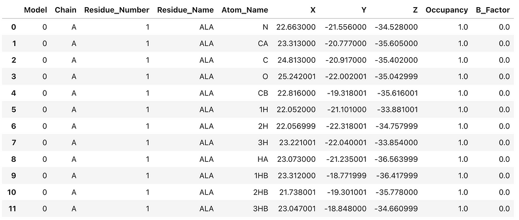
When creating protein structure network (PSN) visualizations, I typically begin by extracting key components from the Protein Data Bank (PDB) structure file using PDBParser from the Biopython package. For clarification, the PDB archive is a publicly accessible database that stores 3D structural data of biological molecules, such as proteins and nucleic acids, for use in scientific research and education. For the purpose of demonstration I am using the PDB structure 4PLD which is a human liver receptor homolog (LRH-1). It is worth noting that the workflow presented here is based on research conducted as part of a drug screening study on LRH-1. Note that you will need to update the line pdb_file = ‘7tt8.pdb’to match the path where your PDB file is stored.
If you’re using a Jupyter Notebook, running this snippet should produce the following output:
This creates a Pandas DataFrame that contains basic atomic information from the crystal structure. To create a 3D network representation of the 4PLD protein structure, we need extract key information from the PDB file. When constructing PSNs I prefer to combine the residue number and name for each node so that on visual inspection the researcher can ‘get a feel’ for how the primary sequence structure is mapped to the network topology. In PSNs each residue is represented as a node. As a rule, I limit the network to chain A and only include C-alpha atoms. Therefore, each residue is represented by that residue’s C-alpha atom and corresponding x,y,z coordinates. The C-alpha coordinates are extracted as node features to construct the 3D network. It’s an exciting and insightful process!
Creating PSNs Using the Residue Interaction Network Generator
The Residue Interaction Network Generator (RING) is an online server that transforms protein structures into network representations. As mentioned earlier, residues are treated as nodes and interactions between them as edges. Generally, an interaction is interpreted in terms of proximity, i.e., Euclidean distances. However, other types of interactions are included, such as hydrogen bonds, salt bridges (ionic bonds), π-π stacking and van der Waals. The RING helps visualize and quantify the topological, or structural, features that emerges from residue-residue interaction network. Quantifying these structural features allows researchers to ask questions about functional hot spots, potential allosteric sites, and signaling pathways which may advance our understanding of protein dynamics and contribute to computational drug repurposing.
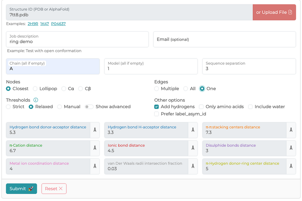
There are other methods for generating PSNs — residue-residue interactions. However, the RING server has been peer-reviewed and provides detailed documentation on how edges are calculated and what defines a connection. Below is a screenshot of a typical configuration I use for generating PSNs. I generally select parameters that I think are maximize edge inclusion. The RING server allows you to either retrieve a structure file from the PDB archive or upload a local file, which is what I have done in this case.
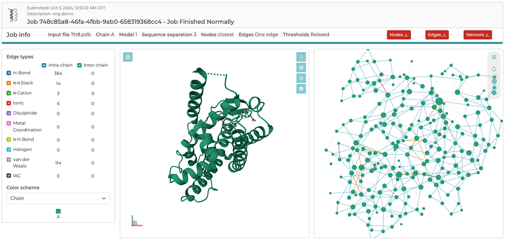
Once the server is finished with its computations, you’ll see an output similar to the screenshot below. Rather than going through the details of the results here, I encourage readers to explore the RING server and become familiar with its output by simply tinkering around. There are three three files that are generated for download: a .cif_ringNodes, a .cif_ringEdges, and a .json file, which contain everything needed to build either a 2D or 3D network. The entire 3D network, including x,y,z coordinates, is contained in the .json file. In a separate post, I will demonstrate how to read the .json file and plot the 3D network using Plotly. Again, the reason I extract coordinates from the PDB file, rather than the coordinates available in the .json file, is to ensure that the edges between residues map to the C-alpha atoms. It is a convention that structural biologists easily recognize and understand.
RING server results
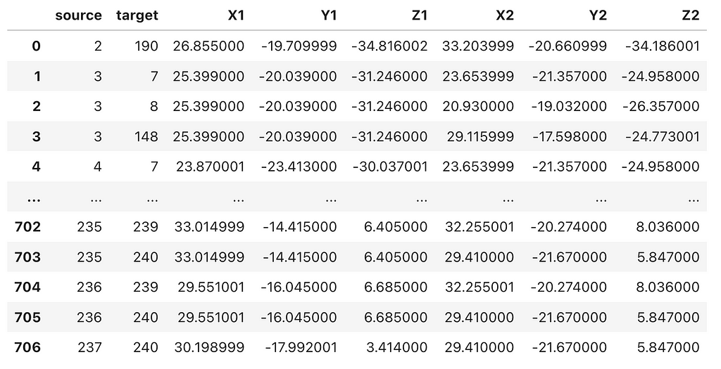
Next, we will import the .cif_ringEdges file downloaded from the RING server into a Pandas DataFrame, and then merge the residue-residue interactions (edges) with the C-alpha atom coordinates from the PDB file.
This should produce a data frame with ‘source’ and ‘target’ node columns, followed by the corresponding x, y, z coordinates for both the ‘source’ and ‘target’ nodes, similar to the example shown below.
Lastly, with the Plotly and NetworkX libraries, we can create a script to generate an interactive 3D network visualization.
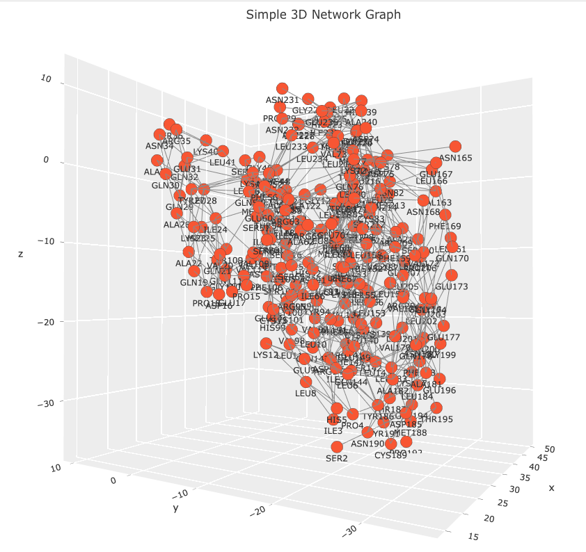
Observe that the code creates a Networkx graph object from the edgelist_7tt8_coords data frame. Please, note that the graph object isn’t necessary to create the 3D network visualization. This code snippet is included for a future post, where the graph object will be used to calculate various measures of centrality which will be mapped to the network’s visual features. The data frame is parsed using standard Python operations. Coordinates for each residue are extracted and with duplicate nodes being removed. Each residue is linked to a text marker in the 3D plot displaying a residue names and sequence position label. Hover labels are also assigned, but note that the label information is redundant. This information was left as a place holder. In a future post I will demonstrate how the hover label can be used to annotate the network with other information such as centrality score, evolutionary conservation score, or links to other databases. The Plotly figure is easily customizable with figure title, axis grids, and node and edge properties. The result is an interactive 3D network that allows users to explore the relationships between residues in any PSN. Images of the 7TT8 PSN are displayed below.
3D protein structure network using Plotly
There’s a lot more we can do with this figure. We can enhance it by adding widgets that dynamically resize nodes based on different centrality measures, or include biological and analytical annotations in the hover information. I’ll explore these enhancements in a future post. You can find the Jupyter Notebook for this exercise on GitHub. If you have any questions, feel free to contact me at [email protected].
Unless otherwise noted, all images are created by the author.
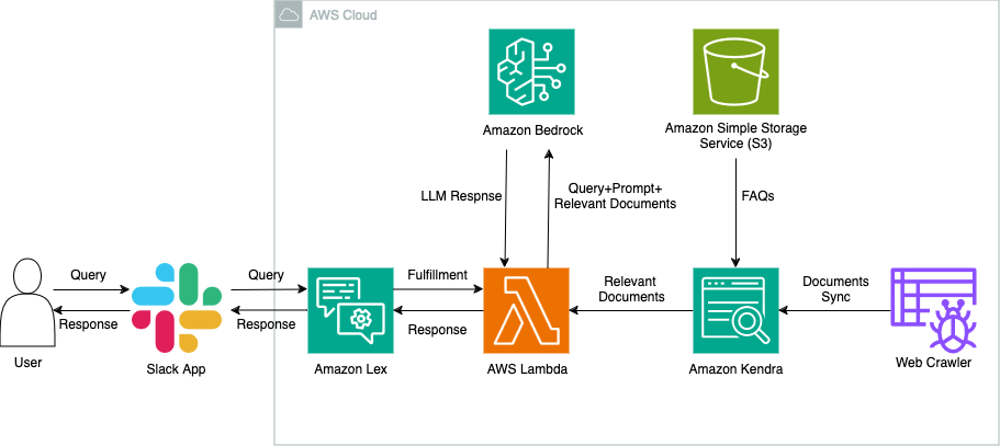
In this post, we describe the development of a generative AI Slack application powered by Amazon Bedrock and Amazon Kendra. This is designed to be an internal-facing Slack chat assistant that helps answer questions related to the indexed content.
Large Language Models (LLMs) have emerged as a transformative force, revolutionizing how we interact with and process information. These powerful AI models, capable of understanding and generating human-like text, have found applications in a wide array of fields, from chatbots and virtual assistants to content creation and data analysis.
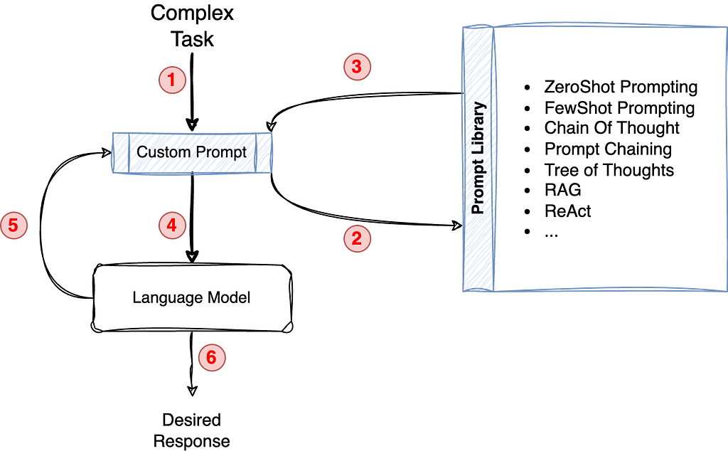
Usual Prompt based development workflow. Source: Author
However, building and maintaining effective LLM-powered applications is not without its challenges. Prompt engineering, the art of crafting precise instructions for LLMs, can be a time-consuming and iterative process. Debugging and troubleshooting LLM behavior can also be complex, given the inherent “black box” nature of these models. Additionally, gaining insights into the performance and cost implications of LLM applications is crucial for optimization and scalability (key components for any production grade setup).
The LLM Ecosystem
The ecosystem for LLMs is still in its nascent stages. To address some of these challenges, a number of innovative tools and frameworks are being developed. DSPy from Stanford University is one such unique take towards formalizing LLM-based app development. Langfuse on the other hand has emerged as an offering to streamline and operationalize aspects of LLM app maintenance. To put it in brief:
DSPY provides a modular and composable framework for building LLM applications, abstracting away the complexities of prompt engineering and enabling developers to focus on the core logic of their applications.
Langfuse offers a comprehensive observability platform for LLM apps, providing deep insights into model performance, cost, and user interactions.
By combining DSPy and Langfuse, developers can unlock the full potential of LLMs, building robust, scalable, and insightful applications that deliver exceptional user experiences.
Unlocking LLM Potential with DSPy
Language Models are extremely complex machines with capabilities to retrieve and reformulate information from an extremely large latent space. To guide this search and achieve desired responses we heavily rely on complex, long and brittle prompts which (at times) are very specific to certain LLMs.
Being an open area of research, teams are working from different perspectives to abstract and enable rapid development of LLM-enabled systems. DSPy is one such framework for algorithmically optimizing LLM prompts and weights.
Ok, You Got Me Intrigued, Tell Me More?
The DSPy framework takes inspiration from deep learning frameworks such as PyTorch.
For instance, to build a deep neural network using PyTorch we simply use standard layers such as convolution, dropout, linear and attach them to optimizers like Adam and train without worrying about implementing these from scratch every time.
Similarly, DSPy provides a a set of standard general purpose modules (such as ChainOfThought,Predict), optimizers (such as BootstrapFewShotWithRandomSearch) and helps us build systems by composing these components as layers into a Program without explicitly dealing with prompts! Neat isn’t it?
The DSPy Building Blocks & Workflow
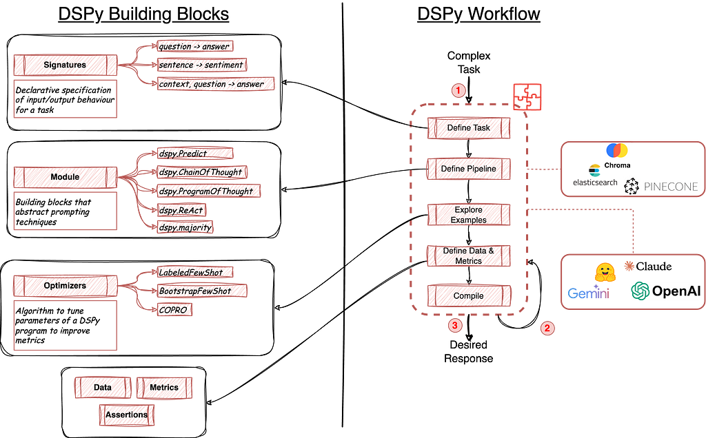
Figure 1: (left) DSPy Building Blocks consisting of Signatures, Modules, Optimizers. (right) DSPy Program workflow. Source: Author
As illustrated in figure 1, DSPy is a pytorch-like/lego-like framework for building LLM-based apps. Out of the box, it comes with:
Signatures: These are specifications to define input and output behaviour of a DSPy program. These can be defined using short-hand notation (like “question -> answer” where the framework automatically understands question is the input while answer is the output) or using declarative specification using python classes (more on this in later sections)
Modules: These are layers of predefined components for powerful concepts like Chain of Thought, ReAct or even the simple text completion (Predict). These modules abstract underlying brittle prompts while still providing extensibility through custom components.
Optimizers: These are unique to DSPy framework and draw inspiration from PyTorch itself. These optimizers make use of annotated datasets and evaluation metrics to help tune/optimize our LLM-powered DSPy programs.
Data, Metrics, Assertions and Trackers are some of the other components of this framework which act as glue and work behind the scenes to enrich this overall framework.
To build an app/program using DSPy, we go through a modular yet step by step approach (as shown in figure 1 (right)). We first define our task to help us clearly define our program’s signature (input and output specifications). This is followed by building a pipeline program which makes use of one or more abstracted prompt modules, language model module as well as retrieval model modules. One we have all of this in place, we then proceed to have some examples along with required metrics to evaluate our setup which are used by optimizers and assertion componentsto compile a powerful app.
Gaining LLM Insights with Langfuse
Langfuse is an LLM Engineering platform designed to empower developers in building, managing, and optimizing LLM-powered applications. While it offers both managed and self-hosting solutions, we’ll focus on the self-hosting option in this post, providing you with complete control over your LLM infrastructure.
Key Highlights of Langfuse Setup
Langfuse equips you with a suite of powerful tools to streamline the LLM development workflow:
Prompt Management: Effortlessly version and retrieve prompts, ensuring reproducibility and facilitating experimentation.
Tracing: Gain deep visibility into your LLM applications with detailed traces, enabling efficient debugging and troubleshooting. The intuitive UI out of the box enables teams to annotate model interactions to develop and evaluate training datasets.
Metrics: Track crucial metrics such as cost, latency, and token usage, empowering you to optimize performance and control expenses.
Evaluation: Capture user feedback, annotate LLM responses, and even set up evaluation functions to continuously assess and improve your models.
Datasets: Manage and organize datasets derived from your LLM applications, facilitating further fine-tuning and model enhancement.
Effortless Setup
Langfuse’s self-hosting solution is remarkably easy to set up, leveraging a docker-based architecture that you can quickly spin up using docker compose. This streamlined approach minimizes deployment complexities and allows you to focus on building your LLM applications.
Framework Compatibility
Langfuse seamlessly integrates with popular LLM frameworks like LangChain, LlamaIndex, and, of course, DSPy, making it a versatile tool for a wide range of LLM development frameworks.
The Power of DSPY + Langfuse
By integrating Langfuse into your DSPy applications, you unlock a wealth of observability capabilities that enable you to monitor, analyze, and optimize your models in real time.
Integrating Langfuse into Your DSPy App
The integration process is straightforward and involves instrumenting your DSPy code with Langfuse’s SDK.
import dspy from dsp.trackers.langfuse_tracker import LangfuseTracker
# dspy predict supercharged with automatic langfuse trackers openai("What is DSPy?")
Gaining Insights with Langfuse
Once integrated, Langfuse provides a number of actionable insights into your DSPy application’s behavior:
Trace-Based Debugging: Follow the execution flow of your DSPY programs, pinpoint bottlenecks, and identify areas for improvement.
Performance Monitoring: Track key metrics like latency and token usage to ensure optimal performance and cost-efficiency.
User Interaction Analysis: Understand how users interact with your LLM app, identify common queries, and opportunities for enhancement.
Data Collection & Fine-Tuning: Collect and annotate LLM responses, building valuable datasets for further fine-tuning and model refinement.
Use Cases Amplified
The combination of DSPy and Langfuse is particularly important in the following scenarios:
Complex Pipelines: When dealing with complex DSPy pipelines involving multiple modules, Langfuse’s tracing capabilities become indispensable for debugging and understanding the flow of information.
Production Environments: In production settings, Langfuse’s monitoring features ensure your LLM app runs smoothly, providing early warnings of potential issues while keeping an eye on costs involved.
Iterative Development: Langfuse’s evaluation and dataset management tools facilitate data-driven iteration, allowing you to continuously refine your LLM app based on real-world usage.
The Meta Use Case: Q&A Bot for my Workshop
To truly showcase the power and versatility of DSPy combined with amazing monitoring capabilities of langfuse, I’ve recently applied them to a unique dataset: my recent LLM workshop GitHub repository. This recent full day workshop contains a lot of material to get you started with LLMs. The aim of this Q&A bot was to assist participants during and after the workshop with answers to a host NLP and LLM related topics covered in the workshop. This “meta” use case not only demonstrates the practical application of these tools but also adds a touch of self-reflection to our exploration.
The Task: Building a Q&A System
For this exercise, we’ll leverage DSPy to build a Q&A system capable of answering questions about the content of my workshop (notebooks, markdown files, etc.). This task highlights DSPy’s ability to process and extract information from textual data, a crucial capability for a wide range of LLM applications. Imagine having a personal AI assistant (or co-pilot) that can help you recall details from your past weeks, identify patterns in your work, or even surface forgotten insights! It also presents a strong case of how such a modular setup can be easily extended to any other textual dataset with little to no effort.
Let us begin by setting up the required objects for our program.
import os import dspy from dsp.trackers.langfuse_tracker import LangfuseTracker
Once we have these clients and trackers in place, let us quickly add some documents to our collection (refer to this notebook for a detailed walk through of how I prepared this dataset in the first place).
# Add to collection
collection.add(
    documents=[v for _,v in nb_scraper.notebook_md_dict.items()],
    ids=doc_ids, # must be unique for each doc
)
The next step is to simply connect our chromadb retriever to the DSPy framework. The following snippet created a RM object and tests if the retrieval works as intended.
# Test Retrieval results = retriever_model("RLHF") for result in results: display(Markdown(f"__Document__::{result.long_text[:100]}... n")) display(Markdown(f">- __Document id__::{result.id} n>- __Document score__::{result.score}"))
The output looks promising given that without any intervention, Chromadb is able to fetch the most relevant documents.
Document::# Quick Overview of RLFH
The performance of Language Models until GPT-3 was kind of amazing as-is. ...
The final step is to piece all of this together in preparing a DSPy program. For our simple Q&A use-case we make prepare a standard RAG program leveraging Chromadb as our retriever and Langfuse as our tracker. The following snippet presents the pytorch-like approach of developing LLM based apps without worrying about brittle prompts!
# RAG Signature class GenerateAnswer(dspy.Signature): """Answer questions with short factoid answers."""
context = dspy.InputField(desc="may contain relevant facts") question = dspy.InputField() answer = dspy.OutputField(desc="often less than 50 words")
# RAG Program class RAG(dspy.Module): def __init__(self, num_passages=3): super().__init__()
# compile a RAG # note: we are not using any optimizers for this example compiled_rag = RAG()
Phew! Wasn’t that quick and simple to do? Let us now put this into action using a few sample questions.
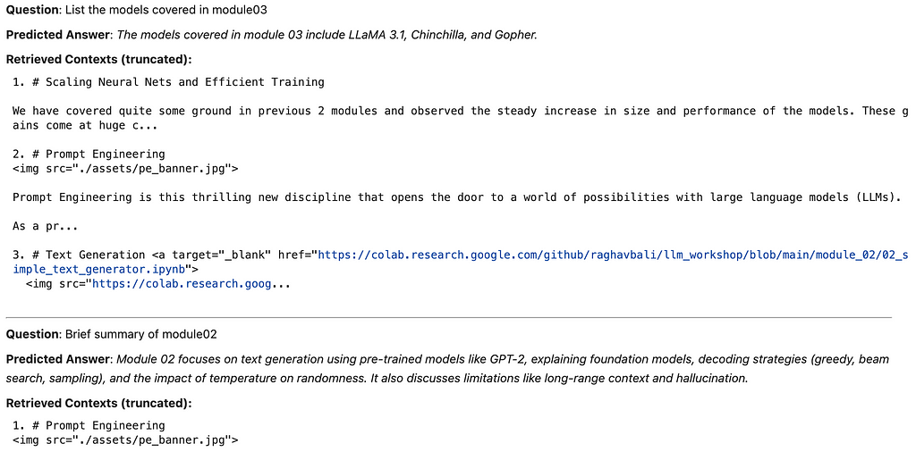
my_questions = [
    "List the models covered in module03",
    "Brief summary of module02",
    "What is LLaMA?"
]

for question in my_questions:
    # Get the prediction. This contains `pred.context` and `pred.answer`.
    pred = compiled_rag(question)

    display(Markdown(f"__Question__: {question}"))
    display(Markdown(f"__Predicted Answer__: _{pred.answer}_"))
    display(Markdown("__Retrieved Contexts (truncated):__"))
    for idx,cont in enumerate(pred.context):
        print(f"{idx+1}. {cont[:200]}..." )
        print()
    display(Markdown('---'))
The output is indeed quite on point and serves the purpose of being an assistant to this workshop material answering questions and guiding the attendees nicely.
Figure 2: Output from the DSPy RAG program. Source: Author
The Langfuse Advantage
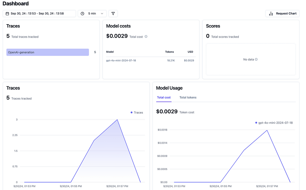
Earlier in this article we discussed how langfuse completes the picture by enabling us to monitor LLM usage and improve upon other aspects of the pipeline. The amazing integration of langfuse as a tracker glues everything behind the scenes with a nice and easy to use interface. For our current setting, the langfuse dashboard presents a quick summary of our LLM usage.
Figure 3: Langfuse Dashboard. Source: Author
The dashboard is complete with metrics such as number of traces, overall costs and even token usage (which is quite handy when it comes to optimize your pipelines).
Insights and Benefits
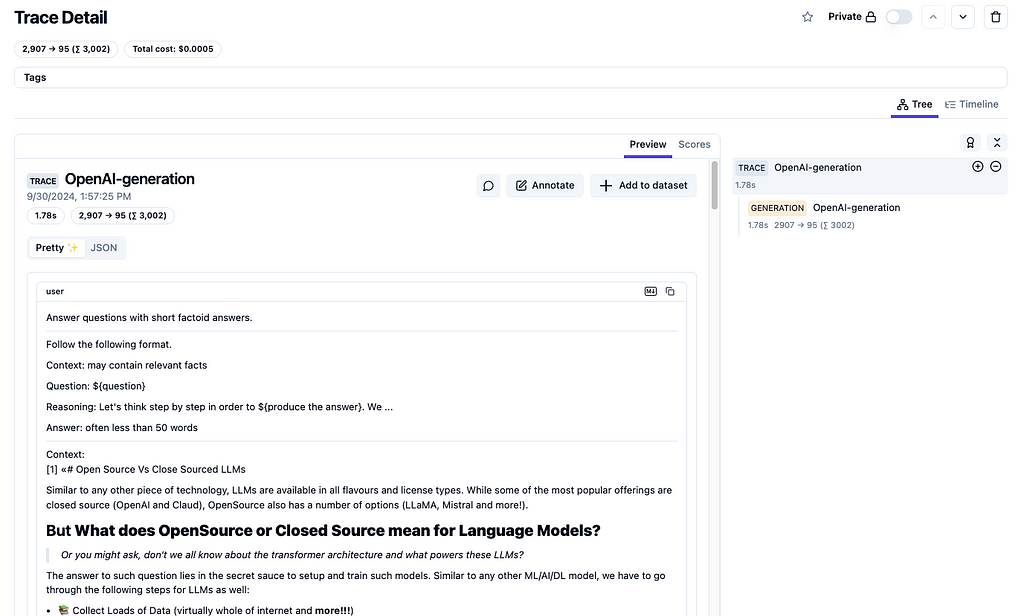
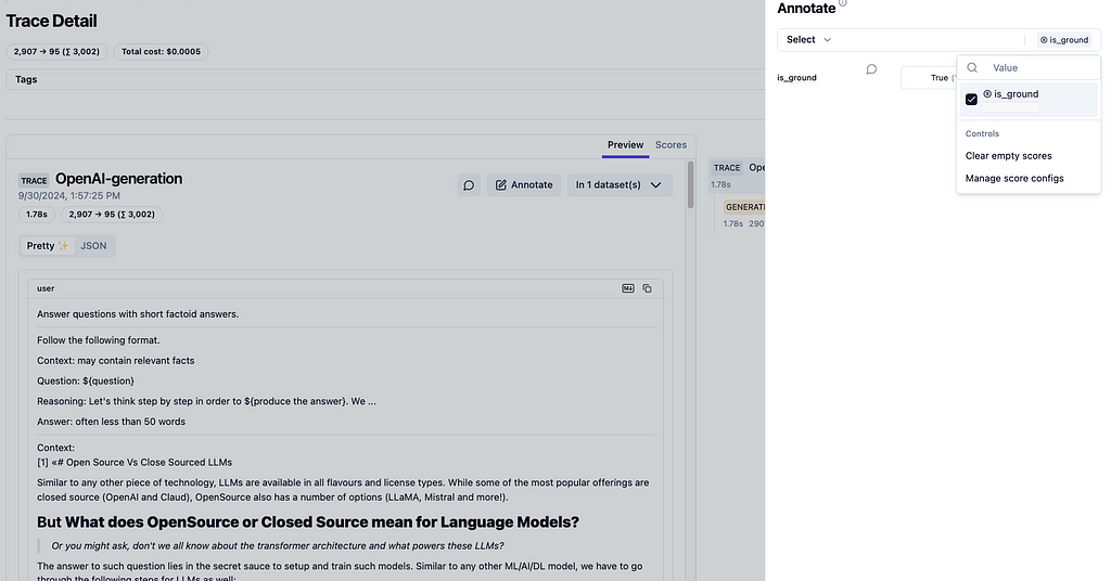
Langfuse’s utility does not end with top-level dashboard of metrics. It provides trace level details (as shown in figure 4).
Figure 4: Langfuse trace detail complete with cost, token usage, prompt as well as the model response. Source: Author.
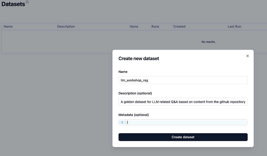
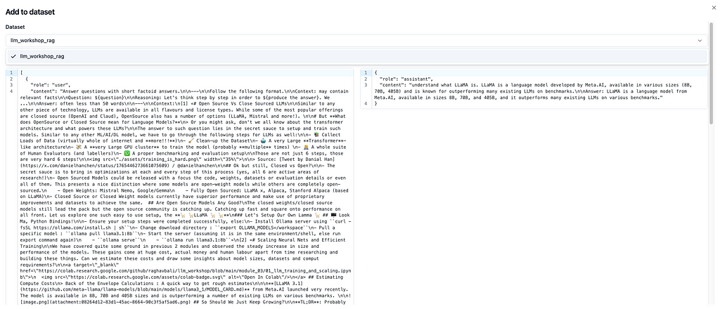
This interface is a gateway to a number of other aspects that are very useful in terms of iterating and improving LLM based apps. The first and foremost capability is to prepare datasets based on real world usage. These datasets can be used for fine-tuning LLMs, optimizing DSPy programs, etc. Figure 5 illustrates how simple it is to define a dataset from the web-UI itself and then add traces (input request along with model’s response) as needed to the dataset.
Figure 5: (left) Create a new dataset from the web UI directly by simply providing the required details such as dataset name and description. (right) traces can be added to datasets at the click of a button. Source: Author
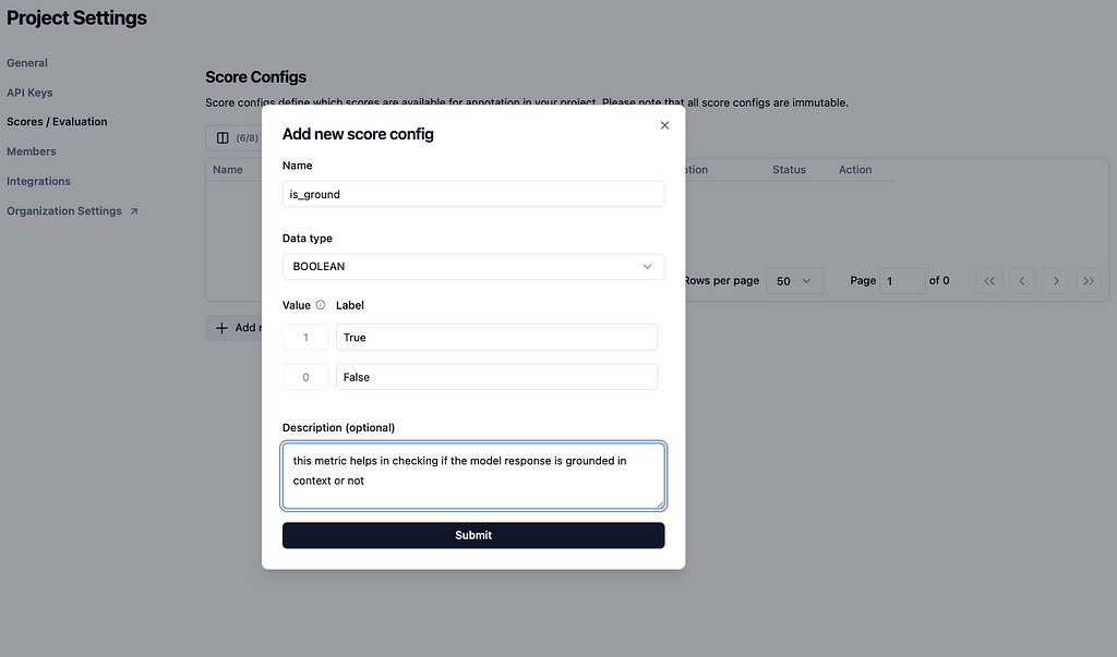
Similar to dataset creation and adding data points to it, langfuse simplifies creation of metrics and annotating datapoints. Figure 6 illustrates how simple it is to do the same at the click of a couple of buttons.
Figure 6: Metric creation and annotation in Langfuse. Source: Author
Once we have a dataset prepared, langfuse provides a straightforward SDK to use it in your language of of preference. The following snippet makes use of get_dataset utility from langfuse to get to a couple of traces we added to the sample dataset. We then use LLaMA 3.1 to power our DSPy RAG program with just one line change (talk about modularity 😉 ).
# get annotated dataset annotated_dataset = langfuse.get_dataset("llm_workshop_rag")
# ensure ollama is available in your environment ollama_dspy = dspy.OllamaLocal(model='llama3.1',temperature=0.5)
# get langfuse client from the dspy tracker object langfuse =langfuse_tracker.langfuse
# Set up the ollama as LM and RM dspy.settings.configure(lm=ollama_dspy,rm=retriever_model)
# test rag using ollama ollama_rag = RAG()
# iterate through samples from the annotated dataset for item in annotated_dataset.items: question = item.input[0]['content'].split('Question: ')[-1].split('n')[0] answer = item.expected_output['content'].split('Answer: ')[-1] o_pred = ollama_rag(question)
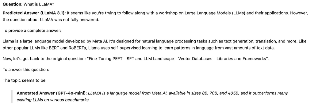
# add observations to dataset related experiments with item.observe( run_name='ollama_experiment', run_description='compare LLaMA3.1 RAG vs GPT4o-mini RAG ', run_metadata={"model": "llama3.1"}, ) as trace_id: langfuse.score( name="visual-eval", # any float value value=1.0, comment="LLaMA3.1 is very verbose", ) # attach trace with new run langfuse.trace(input=question,output=o_pred.answer,metadata={'model':'LLaMA3.1'}) display(Markdown(f"__Question__: {question}")) display(Markdown(f"__Predicted Answer (LLaMA 3.1)__: {o_pred.answer}")) display(Markdown(f">__Annotated Answer (GPT-4o-mini)__: _{answer}_"))
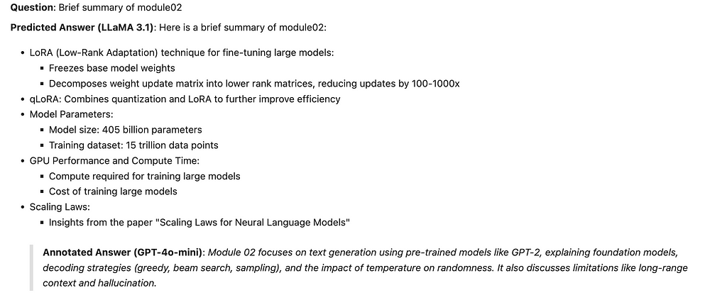
As shown in the above snippet, we simply iterate through the datapoints in our dataset and visually compare the output from both models (see figure 7). Using Langfuse SDK we attach experiment observations along with new traces and evaluation scores very easily.
Figure 7: Output from LLaMA3.1 powered RAG using datapoints from dataset prepared using Langfuse
The output presented in figure 7 clearly shows how LLaMA3.1 powered RAG does answer the questions but strays from the instructions of being brief. This can be easily captured using DSPy assertions as well as scores can be tracked using langfuse SDK for further improvements.
Conclusion
In this rapidly evolving landscape of LLM applications, tools like DSPy and Langfuse emerge as invaluable allies for developers & data scientists. DSPy streamlines the development process, empowering you to build sophisticated LLM applications with ease and efficiency. Meanwhile, Langfuse provides the crucial observability layer, enabling you to gain deep insights into your models’ performance, optimize resource utilization, and continuously improve your applications based on real-world data.
The combination of DSPY and Langfuse unlocks a world of possibilities, allowing you to harness the full potential of LLMs. Whether you’re building Q&A systems, content generators, or any other LLM-powered application, these tools provide the foundation for creating robust, scalable, and insightful solutions.
As I’ve demonstrated through the meta usecase of answering questions for my recent LLM-workshop, DSPy and Langfuse can be applied creatively to extract valuable insights from even your own personal data. The possibilities are truly endless.
I encourage you to explore these tools/frameworks in your own projects. Interested folks can leverage the comprehensive hands-on driven workshop material for more topics on my GitHub repository. With these tools at your disposal, you’re well-equipped to supercharge your LLM applications and stay ahead in the ever-evolving world of AI.
Common challenges and architectural components to enable scaling
Source: Generated with the help of AI (OpenAI’s Dall-E model)
1. Introduction
1.1. Overview of RAG
Those of you who have been immersed in generative AI and its large-scale applications outside of personal productivity apps have likely come across the notion of Retrieval Augmented Generation or RAG. The RAG architecture consists of two key components—the retrieval component which uses vector databases to do an index based search on a large corpus of documents. This is then sent over to a large language model (LLM) to generate a grounded response based on the richer context in the prompt.
Whether you are building customer-facing chatbots to answer repetitive questions and reduce workload from customer service agents, or building a co-pilot for engineers to help them navigate complex user manuals step-by-step, RAG has become a key archetype of the application of LLMs. This has enabled LLMs to provide a contextually relevant response based on ground truth of hundreds or millions of documents, reducing hallucinations and improving the reliability of LLM-based applications.
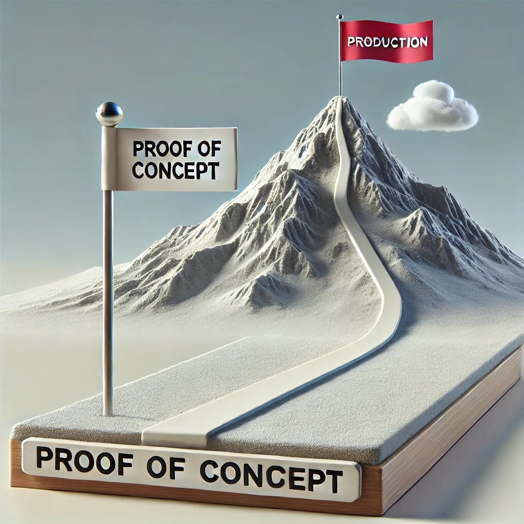
1.2. Why scale from Proof of Concept(POC) to production
If you are asking this question, I might challenge you to answer why are you even building a POC if there is no intent of getting it to production. Pilot purgatory is a common risk with organisations that start to experiment, but then get stuck in experimentation mode. Remember that POCs are expensive, and true value realisation only happens once you go into production and do things at scale- either freeing up resources, making them more efficient, or creating additional revenue streams.
2. Key challenges in scaling RAG
2.1. Performance
Performance challenges in RAGs come in various flavours. The speed of retrieval is generally not the primary challenge unless your knowledge corpus has millions of documents, and even then it can be solved by setting up the right infrastructure- of course, we are limited by inference times. The second performance problem we encounter is around getting the “right” chunks to be fed to the LLMs for generation, with a high level of precision and recall. The poorer the retrieval process is, the less contextually relevant the LLM response will be.
2.2. Data Management
We have all heard the age-old saying “garbage in garbage out (GIGO)”. RAG is nothing but a set of tools we have at our disposal, but the real value comes from the actual data. As RAG systems work with unstructured data, it comes with its own set of challenges including but not limited to- version control of documents, and format conversion (e.g. pdf to text), among others.
2.3. Risk
One of the biggest reasons corporations hesitate to move from testing the waters to jumping in is the possible risks that come with using AI based systems. Hallucinations are definitely lowered with the use of RAG, but are still non-zero. There are other associated risks including risks for bias, toxicity, regulatory risks etc. which could have long term implications.
2.4. Integration into existing workflows
Building an offline solution is easier, but bringing in the end users’ perspective is crucial to make sure the solution does not feel like a burden. No users want to go to another screen to use the “new AI feature”- users want the AI features built into their existing workflows so the technology is assistive, and not disruptive to the day-to-day.
2.5. Cost
Well, this one seems sort of obvious, doesn’t it? Organisations are implementing GenAI use cases so that they can create business impact. If the benefits are lower than we planned, or there are cost overruns, the impact would be severely diminished, or also completely negated.
3. Architectural components needed for Scaling
It would be unfair to only talk about challenges if we don’t talk about the “so what do we do”. There are a few essential components you can add to your architecture stack to overcome/diminish some of the problems we outlined above.
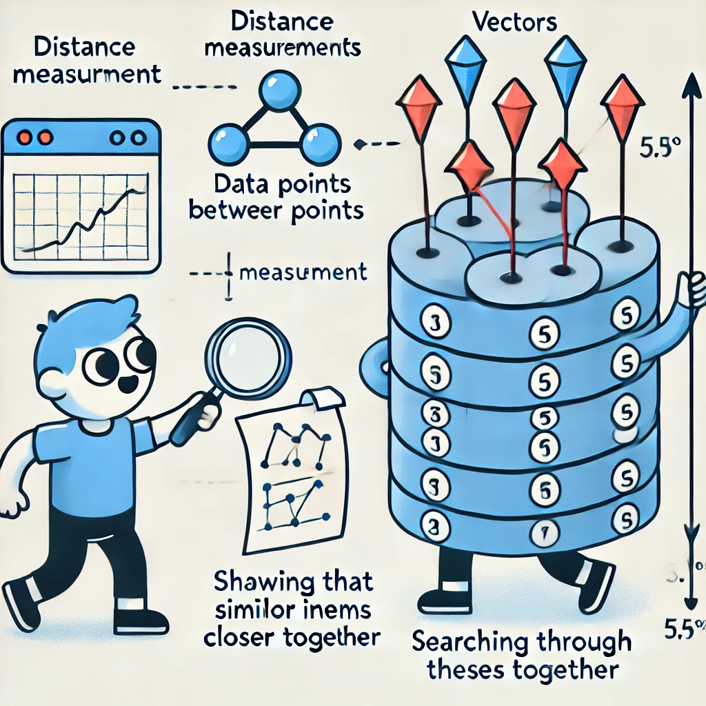
3.1. Scalable vector databases
A lot of teams, rightfully, start with open-source vector databases like ChromaDB, which are great for POCs as they are easy to use and customise. However, it may face challenges with large-scale deployments. This is where scalable vector databases come in (such as Pinecone, Weaviate, Milvus, etc.) which are optimised for high-dimensional vector searches, enabling fast (sub-millisecond), accurate retrieval even as the dataset size increases into the millions or billions of vectors as they use Approximate Nearest Neighbour search techniques. These vector databases have APIs, plugins, and SDKs that allow for easier workflow integration and they are also horizontally scalable. Depending on the platform one is working on- it might make sense to explore vector databases offered by Databricks or AWS.
Source: Generated with the help of AI (OpenAI’s Dall-E model)
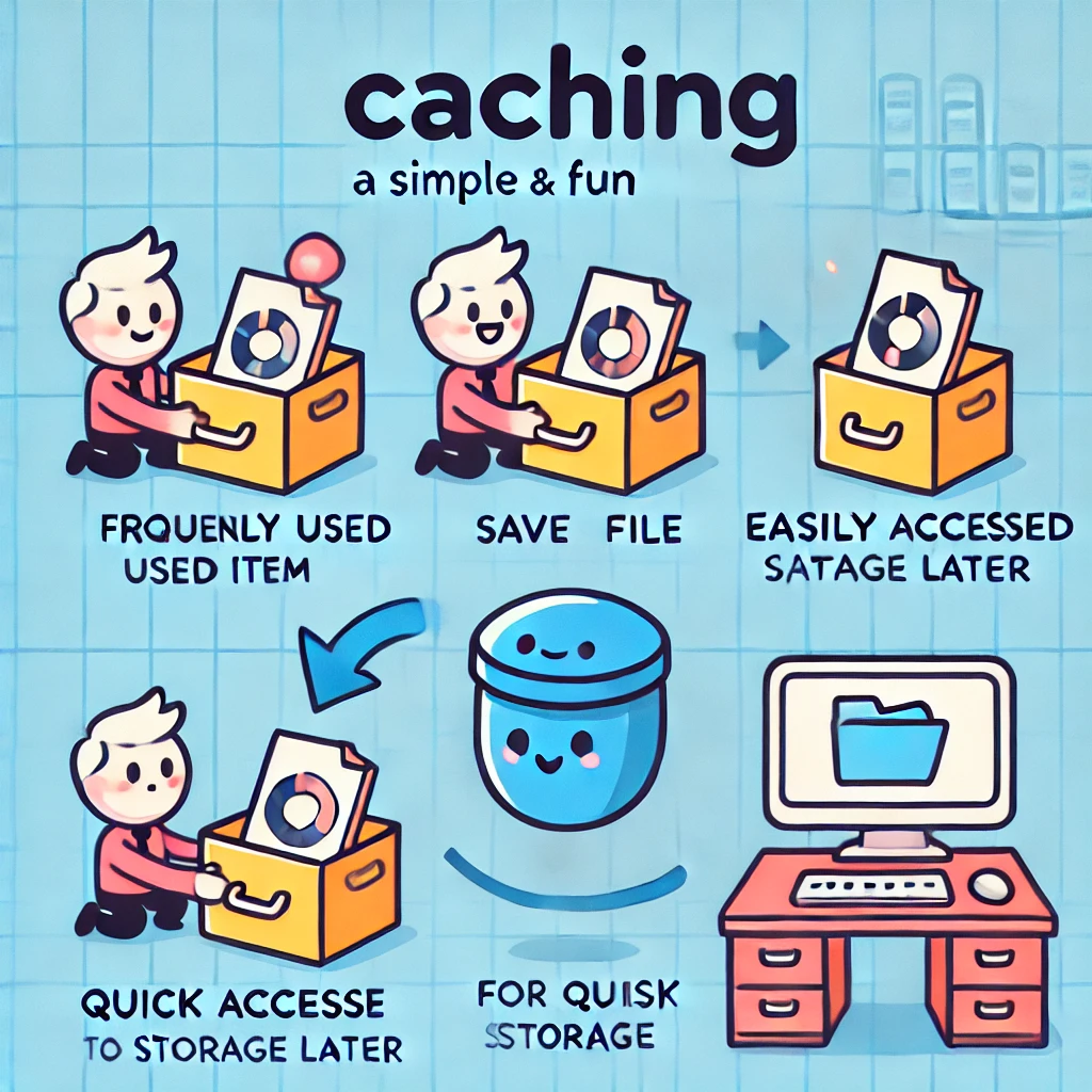
3.2. Caching Mechanisms
The concept of caching has been around almost as long as the internet, dating back to the 1960’s. The same concept applies to GenerativeAI as well—If there are a large number of queries, maybe in the millions (very common in the customer service function), it is likely that many queries are the same or extremely similar. Caching allows one to avoid sending a request to the LLM if we can instead return a response from a recent cached response. This serves two purposes- reduced costs, as well as better response times for common queries.
This can be implemented as a memory Cache (in-memory caches like Redis or Memcached), Disk Cache for less frequent queries or distributed Cache (Redis Cluster). Some model providers like Anthropic offer prompt caching as part of their APIs.
Source: Generated with the help of AI (OpenAI’s Dall-E model)
3.3. Advanced Search Techniques
While not as crisply an architecture component, multiple techniques can help elevate the search to enhance both efficiency and accuracy. Some of these include:
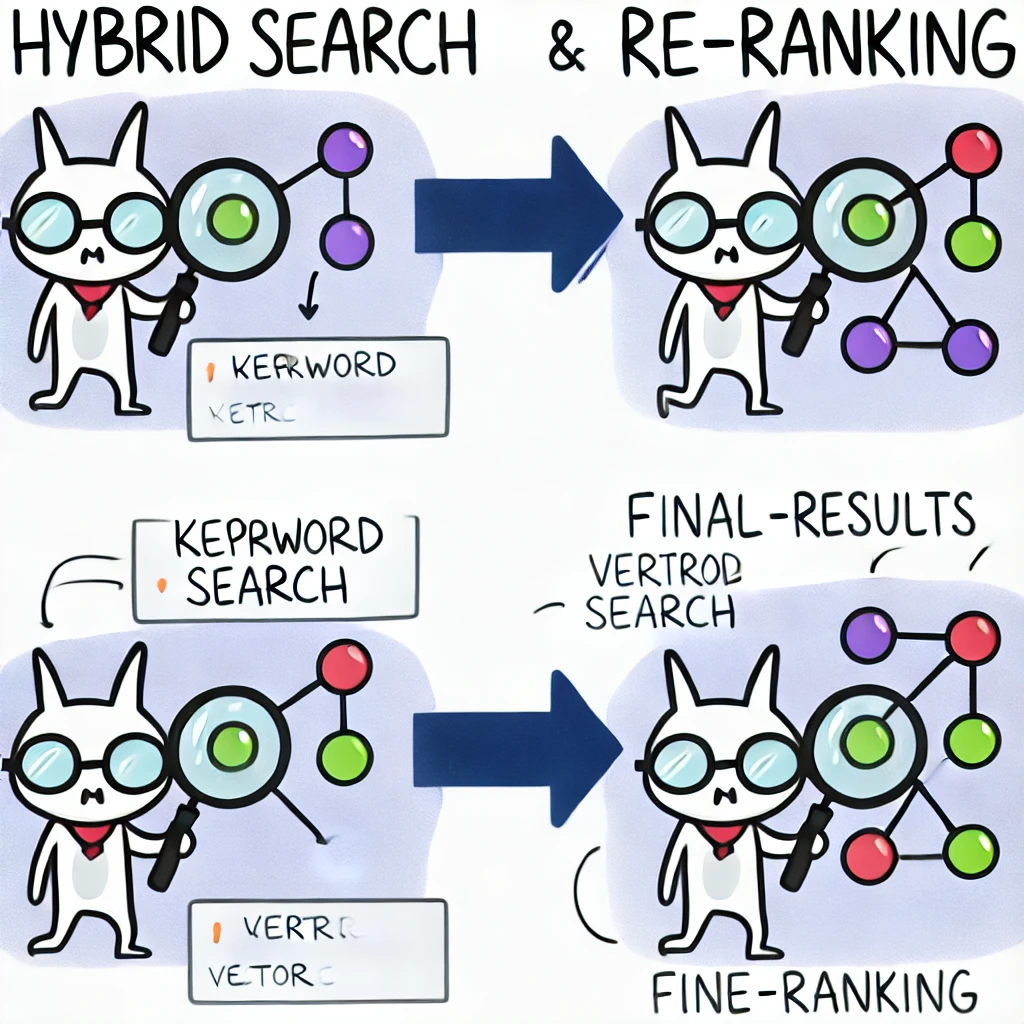
Hybrid Search: Instead of relying only on semantic search(using vector databases), or keyword search, use a combination to boost your search.
Re-ranking: Use a LLM or SLM to calculate a relevancy score for the query with each search result, and re-rank them to extract and share only the highly relevant ones. This is particularly useful for complex domains, or domains where one may have many documents being returned. One example of this is Cohere’s Rerank.
Source: Generated with the help of AI (OpenAI’s Dall-E model)
3.4. Responsible AI layer
Your Responsible AI modules have to be designed to mitigate bias, ensure transparency, align with your organisation’s ethical values, continuously monitor for user feedback and track compliance to regulation among other things, relevant to your industry/function. There are many ways to go about it, but fundamentally this has to be enabled programmatically, with human oversight. A few ways it can be done that can be done:
Pre-processing: Filter user queries before they are ever sent over to the foundational model. This may include things like checking for bias, toxicity, un-intended use etc.
Post-processing: Apply another set of checks after the results come back from the FMs, before exposing them to the end users.
These checks can be enabled as small reusable modules you buy from an external provider, or build/customise for your own needs. One common way organisations have approached this is to use carefully engineered prompts and foundational models to orchestrate a workflow and prevent a result reaching the end user till it passes all checks.
Source: Generated with the help of AI (OpenAI’s Dall-E model)
3.5. API Gateway
An API Gateway can serve multiple purposes helping manage costs, and various aspects of Responsible AI:
Provide a unified interface to interact with foundational models, experiment with them
Help develop a fine-grained view into costs and usage by team/use case/cost centre — including rate-limiting, speed throttling, quota management
Serve as a responsible AI layer, filtering out in-intended requests/data before they ever hit the models
Enable audit trails and access control
Source: Generated with the help of AI (OpenAI’s Dall-E model)
4. Is this enough, or do we need more?
Of course not. There are a few other things that also need to be kept in mind, including but not limited to:
Does the use case occupy a strategic place in your roadmap of use cases? This enables you to have leadership backing, and right investments to support the development and maintenance.
A clear evaluation criterion to measure the performance of the application, against dimensions of accuracy, cost, latency and responsible AI
Improve business processes to keep knowledge up to date, maintain version control etc.
Architect the RAG system so that it only accesses documents based on the end user permission levels, to prevent unauthorised access.
Use design thinking to integrate the application into the workflow of the end user e.g. if you are building a bot to answer technical questions over Confluence as the knowledge base, should you build a separate UI, or integrate this with Teams/Slack/other applications users already use?
5. Conclusion
RAGs are a prominent use case archetype, and one of the first few ones that organisations try to implement. Scaling RAG from POC to production comes with its challenges, but with careful planning and execution, many of these can be overcome. Some of these can be solved by tactical investment in the architecture and technology, some require better strategic direction and tactful planning. As LLM inference costs continue to drop, either owing to reduced inference costs or heavier adoption of open-source models, cost barriers may not be a concern for many new use cases.
Setting up a Voice Agent using Twilio and the OpenAI Realtime API
Introduction
At the recent OpenAI Dev Day on October 1st, 2024, OpenAI’s biggest release was the reveal of their Realtime API:
“Today, we’re introducing a public beta of the Realtime API, enabling all paid developers to build low-latency, multimodal experiences in their apps.
Similar to ChatGPT’s Advanced Voice Mode, the Realtime API supports natural speech-to-speech conversations using the six preset voices already supported in the API.”
(source: OpenAI website)
As per their message, some of its key benefits include low latency, and its speech to speech capabilities. Let’s see how that plays out in practice in terms of building out voice AI agents.
It also has an interruption handling feature, so that the realtime stream will stop sending audio if it detects you are trying to speak over it, a useful feature for sure when building voice agents.
Contents
In this article we will:
Compare what a phone voice agent flow might have looked like before the Realtime API, and what it looks like now,
Review a GitHub project from Twilio that sets up a voice agent using the new Realtime API, so we can see what the implementation looks like in practice, and get an idea how the websockets and connections are setup for such an application,
Quickly review the React demo project from OpenAI that uses the Realtime API,
Compare the pricing of these various options.
Voice Agent Flows
Before the OpenAI Realtime API
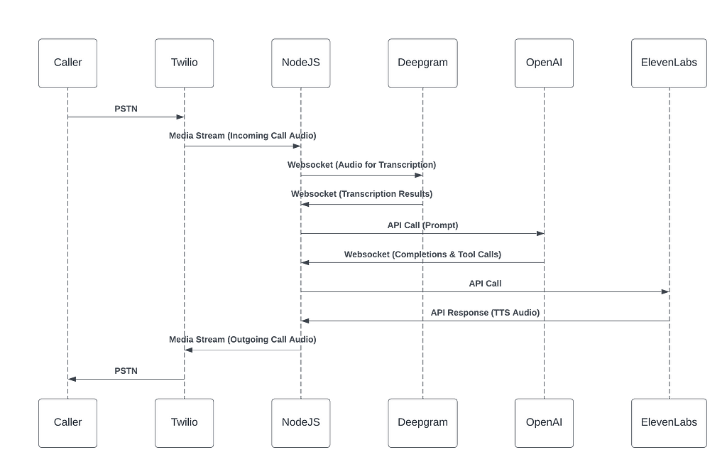
To get a phone voice agent service working, there are some key services we require
Speech to Text ( e.g Deepgram),
LLM/Agent ( e.g OpenAI),
Text to Speech (e.g ElevenLabs).
These services are illustrated in the diagram below
That of course means integration with a number of services, and separate API requests for each parts.
The new OpenAI Realtime API allows us to bundle all of those together into a single request, hence the term, speech to speech.
After the OpenAI Realtime API
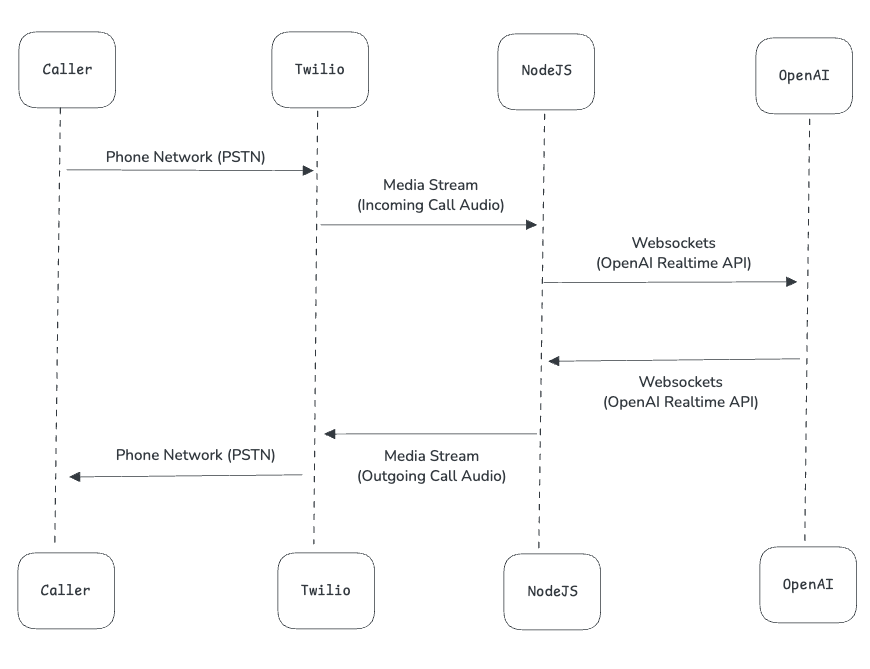
This is what the flow diagram would look like for a similar new flow using the new OpenAI Realtime API.
Obviously this is a much simpler flow. What is happening is we are just passing the speech/audio from the phone call directly to the OpenAI Realtime API. No need for a speech to text intermediary service.
And on the response side, the Realtime API is again providing an audio stream as the response, which we can send right back to Twilio (i.e to the phone call response). So again, no need for an extra text to speech service, as it is all taken care of by the OpenAI Realtime API.
Source code review for a Twilio and Realtime API voice agent
Let’s look at some code samples for this. Twilio has provided a great github repository example for setting up this Twilio and OpenAI Realtime API flow. You can find it here:
Here are some excerpts from key parts of the code related to setting up
the websockets connection from Twilio to our application, so that we can receive audio from the caller, and send audio back,
and the websockets connection to the OpenAI Realtime API from our application.
I have added some comments in the source code below to try and explain what is going on, expecially regarding the websocket connection between Twilio and our applicaion, and the websocket connection from our application to OpenAI. The triple dots (…) refere to sections of the source code that have been removed for brevity, since they are not critical to understanding the core features of how the flow works.
// On receiving a phone call, Twilio forwards the incoming call request to // a webhook we specify, which is this endpoint here. This allows us to // create programatic voice applications, for example using an AI agent // to handle the phone call // // So, here we are providing an initial response to the call, and creating // a websocket (called a MediaStream in Twilio, more on that below) to receive // any future audio that comes into the call fastify.all('/incoming', async (request, reply) => { const twimlResponse = `<?xml version="1.0" encoding="UTF-8"?> <Response> <Say>Please wait while we connect your call to the A. I. voice assistant, powered by Twilio and the Open-A.I. Realtime API</Say> <Pause length="1"/> <Say>O.K. you can start talking!</Say> <Connect> <Stream url="wss://${request.headers.host}/media-stream" /> </Connect> </Response>`;
reply.type('text/xml').send(twimlResponse); });
fastify.register(async (fastify) => {
// Here we are connecting our application to the websocket media stream we // setup above. That means all audio that comes though the phone will come // to this websocket connection we have setup here fastify.get('/media-stream', { websocket: true }, (connection, req) => { console.log('Client connected');
// Now, we are creating websocket connection to the OpenAI Realtime API // This is the second leg of the flow diagram above const openAiWs = new WebSocket('wss://api.openai.com/v1/realtime?model=gpt-4o-realtime-preview-2024-10-01', { headers: { Authorization: `Bearer ${OPENAI_API_KEY}`, "OpenAI-Beta": "realtime=v1" } });
...
// Here we are setting up the listener on the OpenAI Realtime API // websockets connection. We are specifying how we would like it to // handle any incoming audio streams that have come back from the // Realtime API. openAiWs.on('message', (data) => { try { const response = JSON.parse(data);
...
// This response type indicates an LLM responce from the Realtime API // So we want to forward this response back to the Twilio Mediat Stream // websockets connection, which the caller will hear as a response on // on the phone if (response.type === 'response.audio.delta' && response.delta) { const audioDelta = { event: 'media', streamSid: streamSid, media: { payload: Buffer.from(response.delta, 'base64').toString('base64') } }; // This is the actual part we are sending it back to the Twilio // MediaStream websockets connection. Notice how we are sending the // response back directly. No need for text to speech conversion from // the OpenAI response. The OpenAI Realtime API already provides the // response as an audio stream (i.e speech to speech) connection.send(JSON.stringify(audioDelta)); } } catch (error) { console.error('Error processing OpenAI message:', error, 'Raw message:', data); } });
// This parts specifies how we handle incoming messages to the Twilio // MediaStream websockets connection i.e how we handle audio that comes // into the phone from the caller connection.on('message', (message) => { try { const data = JSON.parse(message);
switch (data.event) { // This case ('media') is that state for when there is audio data // available on the Twilio MediaStream from the caller case 'media': // we first check out OpenAI Realtime API websockets // connection is open if (openAiWs.readyState === WebSocket.OPEN) { const audioAppend = { type: 'input_audio_buffer.append', audio: data.media.payload }; // and then forward the audio stream data to the // Realtime API. Again, notice how we are sending the // audio stream directly, not speech to text converstion // as would have been required previously openAiWs.send(JSON.stringify(audioAppend)); } break;
fastify.listen({ port: PORT }, (err) => { if (err) { console.error(err); process.exit(1); } console.log(`Server is listening on port ${PORT}`); });
So, that is how the new OpenAI Realtime API flow plays out in practice.
Regarding the Twilio MediaStreams, you can read more about them here. They are a way to setup a websockets connection between a call to a Twilio phone number and your application. This allows streaming of audio from the call to and from you application, allowing you to build programmable voice applications over the phone.
To get to the code above running, you will need to setup a Twilio number and ngrok also. You can check out my other article over here for help setting those up.
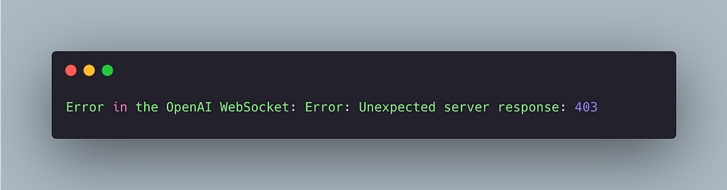
Since access to the OpenAI Realtime API has just been rolled, not everyone may have access just yet. I intially was not able to access it. Running the application worked, but as soon as it tries to connect to the OpenAI Realtime API I got a 403 error. So in case you see the same issue, it could be related to not having access yet also.
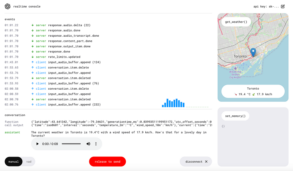
React OpenAI Realtime API Demo
OpenAI have also provided a great demo for testing out their Realtime API in the browser using a React app. I tested this out myself, and was very impressed with the speed of response from the voice agent coming from the Realtime API. The response is instant, there is no latency, and makes for a great user experience. I was definitley impressed when testing it out.
Sharing a link to the source code here. It has intructions in the README.md for how to get setup
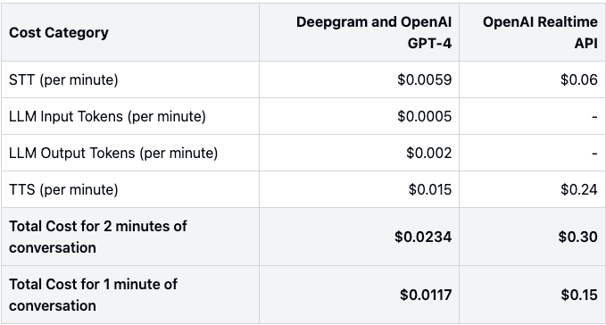
Let’s compare the cost the of using the OpenAI Realtime API versus a more conventional approach using Deepagram for speech to text (STT) and text to speech (TTS) and using OpenAI GPT-4o for the LLM part.
Comparison using the prices from their websites shows that for a 1 minute conversation, with the caller speaking half the time, and the AI agent speaking the other half, the cost per minute using Deepgram and GPT-4o would be $0.0117/minute, whereas using the OpenAI Realtime API would be $0.15/minute.
That means using the OpenAI Realtime API would be just over 10x the price per minute.
It does sound like a fair amount more expensive, though we should balance that with some of the benefits the OpenAI Realtime API could provide, including
reduced latencies, crucial for having a good voice experience,
ease of setup due to fewer moving parts,
conversation interruption handling provided out of the box.
Also, please do be aware that prices can change over time, so the prices you find at the time of reading this article, may not be the same as those reflected above.
Conclusion
Hope that was helpful! What do you think of the new OpenAI Realtime API? Think you will be using it in any upcoming projects?
While we are here, are there any other tutorials or articles around voice agents andvoice AI you would be interested in? I am deep diving into that field a bit just now, so would be happy to look into anything people find interesting.
Happy hacking!
All image provided are by the author, unless stated otherwise
AlphaFold 2 and BERT were both developed in the cradle of Google’s deeply lined pockets in 2018 (albeit by different departments: DeepMind and Google AI). They represented huge leaps forward in state-of-the-art models for natural language processing (NLP) and biology respectively. For BERT, this meant topping the leaderboard on benchmarks like GLUE (General Language Understanding Evaluation) and SQuAD (Stanford Question Answering Dataset). For AlphaFold 2 (hereafter just referred to as AlphaFold), it meant achieving near-experimental accuracy in predicting 3D protein structures. In both cases, these advancements were largely attributed to the use of transformer architecture and the self-attention mechanism.
I expect most machine learning engineers have a cursory understanding of how BERT or Bidirectional encoder representations from transformers work with language but only a vague metaphorical understanding of how the same architecture is applied to the field of biology. The purpose of this article is to explain the concepts behind the development and success of AlphaFold through the lens of how they compare and contrast to BERT.
Forewarning: I am a machine learning engineer and not a biologist, just a curious person.
BERT Primer
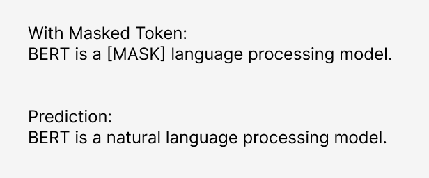
Before diving into protein folding, let’s refresh our understanding of BERT. At a high level, BERT is trained by masked token prediction and next-sentence prediction.
Example masked token prediction where “natural” was the masked token in the target sentence. (All images, unless otherwise noted, are by the author)
BERT falls into the sequence model family. Sequence models are a class of machine learning models designed to handle and make sense of sequential data where the order of the elements matters. Members of the family include Recurrent Neural Nets (RNNs), LSTMs (Long Short Term Memory), and Transformers. As a Transformer model (like its more famous relative, GPT), a key unlock for BERT was how training could be parallelized. RNNs and LSTMs process sequences sequentially, which slows down training and limits the applicable hardware. Transformer models utilize the self-attention mechanism which processes the entire sequence in parallel and allows training to leverage modern GPUs and TPUs, which are optimized for parallel computing.
Processing the entire sequence at once not only decreased training time but also improved embeddings by modeling the contextual relationships between words. This allows the model to better understand dependencies, regardless of their position in the sequence. A classic example illustrates this concept: “I went fishing by the river bank” and “I need to deposit money in the bank.” To readers, bank clearly represents two distinct concepts, but previous models struggled to differentiate them. The self-attention mechanism in transformers enables the model to capture these nuanced differences. For a deeper dive into this topic, I recommend watching this Illustrated Guide to Transformers Neural Network: A step by step explanation.
Example sentences where previous NLP models would have failed to differentiate the two meanings of bank and river bank.
One reason RNNs and LSTMs struggle is because they are unidirectional i.e. they process a sentence from left to right. So if the sentence was rewritten “At the bank, I need to deposit money”, money would no longer clarify the meaning of bank. The self-attention mechanism eliminates this fragility by allowing each word in the sentence to “attend” to every other word, both before and after it making it “bidirectional”.
AlphaFold and BERT Comparison
Now that we’ve reviewed the basics of BERT, let’s compare it to AlphaFold. Like BERT, AlphaFold is a sequence model. However, instead of processing words in sentences, AlphaFold’s inputs are amino acid sequences and multiple sequence alignments (MSAs), and its output/prediction is the 3D structure of the protein.
Let’s review what these inputs and outputs are before learning more about how they are modeled.
First input: Amino Acid Sequences
Amino acid sequences are embedded into high-dimensional vectors, similar to how text is embedded in language models like BERT.
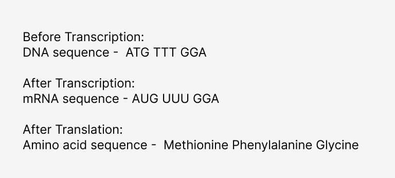
Reminder from your high school biology class: the specific sequence of amino acids that make up a protein is determined by mRNA. mRNA is transcribed from the instructions in DNA. As the amino acids are linked together, they interact with one another through various chemical bonds and forces, causing the protein to fold into a unique three-dimensional structure. This folded structure is crucial for the protein’s function, as its shape determines how it interacts with other molecules and performs its biological roles. Because the 3D structure is so important for determining the protein’s function, the “protein folding” problem has been an important research problem for the last half-century.
Bio 101 reminder on the relationship between DNA, mRNA, and Amino Acid Sequences
Before AlphaFold, the only reliable way to determine how an amino acid sequence would fold was through experimental validation through techniques like X-ray crystallography, NMR spectroscopy (nuclear magnetic resonance), and Cryo-electron microscopy (cryo-EM). Though accurate, these methods are time-consuming, labor-intensive, and expensive.
So what is an MSA (multiple sequence alignment) and why is it another input into the model?
Second input: Multiple sequence alignments, represented as matrices in the model.
Amino acid sequences contain the necessary instructions to build a protein but also include some less important or more variable regions. Comparing this to language, I think of these less important regions as the “stop words” of protein folding instructions. To determine which regions of the sequence are the analogous stop words, MSAs are constructed using homologous (evolutionarily related) sequences of proteins with similar functions in the form of a matrix where the target sequence is the first row.
Similar regions of the sequences are thought to be “evolutionarily conserved” (parts of the sequence that stay the same). Highly conserved regions across species are structurally or functionally important (like active sites in enzymes). My imperfect metaphor here is to think about lining up sentences from Romance languages to identify shared important words. However, this metaphor doesn’t fully explain why MSAs are so important for predicting the 3D structure. Conserved regions are so critical because they allow us to detect co-evolution between amino acids. If two residues tend to mutate in a coordinated way across different sequences, it often means they are physically close in the 3D structure and interact with each other to maintain protein stability. This kind of evolutionary relationship is difficult to infer from a single amino acid sequence but becomes clear when analyzing an MSA.
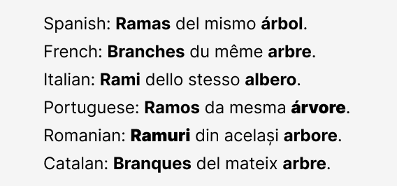
An imperfect metaphor for MSAs: Like comparing similar words in Romance languages (e.g., “branches”: ramas, branches, rami, ramos, ramuri, branques), MSAs align sequences to reveal evolutionary connections, tracing shared origins through small variations.
Here is another place where the comparison of natural language processing and protein folding diverges; MSAs must be constructed and researchers often manually curate them for optimal results. Biologists use tools like BLAST (Basic Local Alignment Search Tool) to search their target sequences to find “homologs” or similar sequences. If you’re studying humans, this could mean finding sequences from other mammals, vertebrates, or more distant organisms. Then the sequences are manually selected considering things like comparable lengths and similar functions. Including too many sequences with divergent functions degrades the quality of the MSA. This is a HUGE difference from how training data is collected for natural language models. Natural language models are trained on huge swaths of data that are hovered up from anywhere and everywhere. Biology models, by contrast, need highly skilled and contentious dataset composers.
What is being predicted/output?
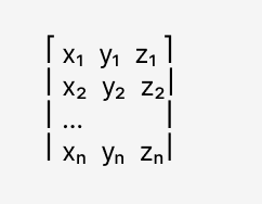
In BERT, the prediction or target is the masked token or next sentence. For AlphaFold, the target is the 3D structure of the protein, represented as the 3D coordinates of protein atoms, which defines the spatial arrangement of amino acids in a folded protein. Each set of 3D coordinates is collected experimentally, reviewed, and stored in the Protein Data Bank. Recently solved structures serve as a validation set for evaluation.
The output of AlphaFold is typically the 3D structure of a protein, which consists of the x, y, z coordinates of the atoms that make up the protein’s amino acids.
How are the inputs and outputs tied together?
Both the target sequence and MSA are processed independently through a series of transformer blocks, utilizing the self-attention mechanism to generate embeddings. The MSA embedding captures evolutionary relationships, while the target sequence embedding documents local context. These contextual embeddings are then fed into downstream layers to predict pairwise interactions between amino acids, ultimately inferring the protein’s 3D structure.
Within each sequence, the pairwise residue (the relationship or interaction between two amino acids within a protein sequence) representation predicts spatial distances and orientations between acids, which are critical for modeling how distant parts of the protein come into proximity when folded. The self-attention mechanism allows the model to account for both local and long-range dependencies within the sequence and MSA. This is important because when a sequence is folded, residues that are far from each other in a sequence may end up close to each other spatially.
The loss function for AlphaFold is considerably more complex than the BERT loss function. BERT faces no spatial or geometric constraints and its loss function is much simpler because it only needs to predict missing words or sentence relationships. In contrast, AlphaFold’s loss function involves multiple aspects of protein structure (distance distributions, torsion angles, 3D coordinates, etc.), and the model optimizes for both ****geometric and spatial predictions. This component heavy loss function ensures that AlphaFold accurately captures the physical properties and interactions that define the protein’s final structure.
While there is essentially no meaningful post-processing required for BERT predictions, predicted 3D coordinates are reviewed for energy minimization and geometric refinement based on the physical principles of proteins. These steps ensure that predicted structures are physically viable and biologically functional.
Conclusion
AlphaFold and BERT both benefit from the transformer architecture and the self-attention mechanism. These improvements improve contextual embeddings and faster training time with GPUs and TPUs.
AlphaFold has a much more complex data preparation process than BERT. Curating MSAs from experimentally derived data is harder than vacuuming up a large corpus of text!
AlphaFold’s loss function must account for spatial or geometric constraints and it’s much more complex than BERT’s.
AlphaFold predictions require post-processing to confirm that the prediction is physically viable whereas BERT predictions do not require post-processing.
Thank you for reading this far! I’m a big believer in cross-functional learning and I believe as machine learning engineers we can learn more by challenging ourselves to learn outside our immediate domains. I hope to continue this series on Understanding AI Applications in Bio for Machine Learning Engineers throughout my maternity leave. ❤
Getting Started with Powerful Data Tables in Your Python Web Apps
Using AG Grid to build a Finance app in pure Python with Reflex
These past few months, I’ve been exploring various data visualization and manipulation tools for web applications. As a Python developer, I often need to handle large datasets and display them in interactive, customizable tables. One question that consistently bothered me was: How can I build a powerful data grid UI that integrates seamlessly with my Python backend?
There are countless options out there to build sophisticated data grids, but as a Python engineer, I have limited experience with JavaScript or any front-end framework. I was looking for a way to create a feature-rich data grid using only the language I’m most comfortable with — Python!
I decided to use Reflex, an open-source framework that lets me build web apps entirely in Python. What’s more, Reflex now offers integration with AG Grid, a feature-rich data grid library designed for displaying and manipulating tabular data in web applications which offers a wide array of functionalities including:
– In-place cell editing
– Real-time data updates
– Pagination and infinite scrolling
– Column filtering, reordering, resizing, and hiding
– Row grouping and aggregation
– Built-in theming
Disclaimer: I work as a Founding Engineer at Reflex where I contribute to the open-source framework.
In this tutorial we will cover how to build a full Finance app from scratch in pure Python to display stock data in an interactive grid and graph with advanced features like sorting, filtering, and pagination — Check out the full live app and code.
Setup
First we import the necessary libraries, including yfinance for fetching the stock data.
import reflex as rx
from reflex_ag_grid import ag_grid
import yfinance as yf
from datetime import datetime, timedelta
import pandas as pd
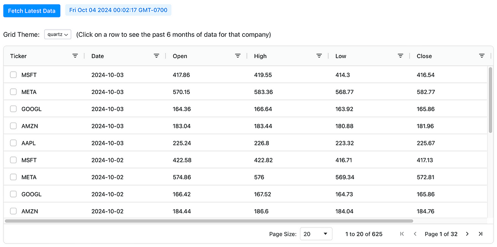
Fetching and transforming data
Next, we define the State class, which contains the application’s state and logic. The fetch_stock_data function fetches stock data for the specified companies and transforms it into a format suitable for display in AG Grid. We call this function when clicking on a button, by linking the on_click trigger of the button to this state function.
We define state variables, any fields in your app that may change over time (A State Var is directly rendered into the frontend of the app).
The data state variable stores the raw stock data fetched from Yahoo Finance. We transform this data to round the values and store it as a list of dictionaries, which is the format that AG Grid expects. The transformed data is sorted by date and ticker in descending order and stored in the dict_data state variable.
The datetime_now state variable stores the current datetime when the data was fetched.
# The list of companies to fetch data for companies = ["AAPL", "MSFT", "GOOGL", "AMZN", "META"]
class State(rx.State): # The data fetched from Yahoo Finance data: pd.DataFrame # The data to be displayed in the AG Grid dict_data: list[dict] = [{}] # The datetime of the current fetched data datetime_now: datetime = datetime.now()
# Fetch data for all tickers in a single download self.data = yf.download(companies, start=start_date, end=self.datetime_now, group_by='ticker') rows = [] for ticker in companies: # Check if the DataFrame has a multi-level column index (for multiple tickers) if isinstance(self.data.columns, pd.MultiIndex): ticker_data = self.data[ticker] # Select the data for the current ticker else: ticker_data = self.data # If only one ticker, no multi-level index exists
The column_defs list defines the columns to be displayed in the AG Grid. The header_name is used to set the header title for each column. The field key represents the id of each column. The filter key is used to insert the filter feature.
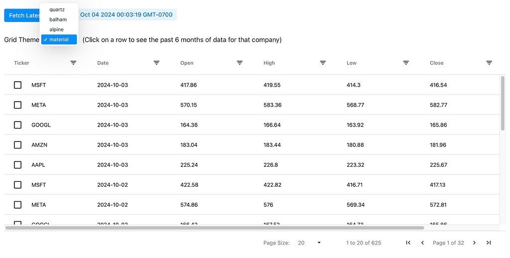
We set theme using the grid_theme State var in the rx.select component.
Every state var has a built-in function to set it’s value for convenience, called set_VARNAME, in this case set_grid_theme.
class State(rx.State): ... # The theme of the AG Grid grid_theme: str = "quartz" # The list of themes for the AG Grid themes: list[str] = ["quartz", "balham", "alpine", "material"]
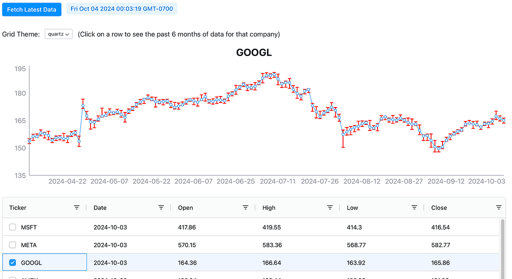
Showing 6 Months of Selected Company Data by Author
The on_selection_changed event trigger, shown in the AG grid code above, is called when the user selects a row in the grid. This calls the function handle_selection method in the State class, which sets the selected_rows state var to the new selected row and calls the function update_line_graph.
The update_line_graph function gets the relevant ticker and uses it to set the company state var. The Date, Mid, and DateDifference data for that company for the past 6 months is then set to the state var dff_ticker_hist.
Finally it is rendered in an rx.recharts.line_chart, using rx.recharts.error_bar to show the DateDifference data which are the highs and the lows for the day.
class State(rx.State): ... # The selected rows in the AG Grid selected_rows: list[dict] = None # The currently selected company in AG Grid company: str # The data fetched from Yahoo Finance data: pd.DataFrame # The data to be displayed in the line graph dff_ticker_hist: list[dict] = None
Using AG Grid inside the Reflex ecosystem empowered me as a Python developer to create sophisticated, data-rich web applications with ease. Whether you’re building complex dashboards, data analysis tools, or an application that demands powerful data grid capabilities, Reflex AG Grid has you covered.
I’m excited to see what you’ll build with Reflex AG Grid! Share your projects, ask questions, and join the discussion in our community forums. Together, let’s push the boundaries of what’s possible with Python web development!
If you have questions, please comment them below or message me on Twitter at @tgotsman12 or on LinkedIn. Share your app creations on social media and tag me, and I’ll be happy to provide feedback or help retweet!
We use cookies on our website to give you the most relevant experience by remembering your preferences and repeat visits. By clicking “Accept”, you consent to the use of ALL the cookies.
This website uses cookies to improve your experience while you navigate through the website. Out of these, the cookies that are categorized as necessary are stored on your browser as they are essential for the working of basic functionalities of the website. We also use third-party cookies that help us analyze and understand how you use this website. These cookies will be stored in your browser only with your consent. You also have the option to opt-out of these cookies. But opting out of some of these cookies may affect your browsing experience.
Necessary cookies are absolutely essential for the website to function properly. These cookies ensure basic functionalities and security features of the website, anonymously.
Cookie
Duration
Description
cookielawinfo-checkbox-analytics
11 months
This cookie is set by GDPR Cookie Consent plugin. The cookie is used to store the user consent for the cookies in the category "Analytics".
cookielawinfo-checkbox-functional
11 months
The cookie is set by GDPR cookie consent to record the user consent for the cookies in the category "Functional".
cookielawinfo-checkbox-necessary
11 months
This cookie is set by GDPR Cookie Consent plugin. The cookies is used to store the user consent for the cookies in the category "Necessary".
cookielawinfo-checkbox-others
11 months
This cookie is set by GDPR Cookie Consent plugin. The cookie is used to store the user consent for the cookies in the category "Other.
cookielawinfo-checkbox-performance
11 months
This cookie is set by GDPR Cookie Consent plugin. The cookie is used to store the user consent for the cookies in the category "Performance".
viewed_cookie_policy
11 months
The cookie is set by the GDPR Cookie Consent plugin and is used to store whether or not user has consented to the use of cookies. It does not store any personal data.
Functional cookies help to perform certain functionalities like sharing the content of the website on social media platforms, collect feedbacks, and other third-party features.
Performance cookies are used to understand and analyze the key performance indexes of the website which helps in delivering a better user experience for the visitors.
Analytical cookies are used to understand how visitors interact with the website. These cookies help provide information on metrics the number of visitors, bounce rate, traffic source, etc.
Advertisement cookies are used to provide visitors with relevant ads and marketing campaigns. These cookies track visitors across websites and collect information to provide customized ads.