Category: Artificial Intelligence

Intuition, step-by-step script, and assumptions needed for the use of IV

In many experiments, not all individuals assigned to receive a treatment actually take it or use it. For example, a company may send discount coupons to customers, intending for them to use these coupons to make a purchase now, which could subsequently increase their future purchases. However, not all customers will redeem the coupon.

This scenario represents “imperfect compliance” (see here), where treatment assignment does not always lead to treatment uptake. To estimate the impact of offering the coupon on future customer purchases, we must distinguish between two main approaches:

• Intention to treat effect (ITT): Estimates the effect of being assigned to receive the coupon, regardless of whether it was used.
• Local average treatment effect (LATE): Estimates the effect of treatment among those who complied with the assignment — those who used the coupon because they were assigned to receive it.

This tutorial introduces the intuition behind these methods, their assumptions, and how to implement them using R (see script here). We will also discuss two-stage least squares (2SLS), the method used to estimate LATE.

Intuition

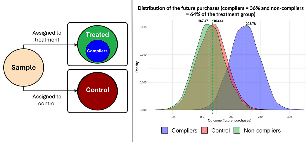
In experiments with imperfect compliance, treatment assignment (e.g., receiving a coupon) does not perfectly correspond to consuming the treatment (e.g., using the coupon). So simply comparing the treatment group to the control group may lead to misleading conclusions, as the effect of the treatment among those who took it (the blue group in the figure below) gets diluted within the larger treatment group (the green group).

To deal with this situation, we use two main approaches:

Intention-to-treat (ITT)

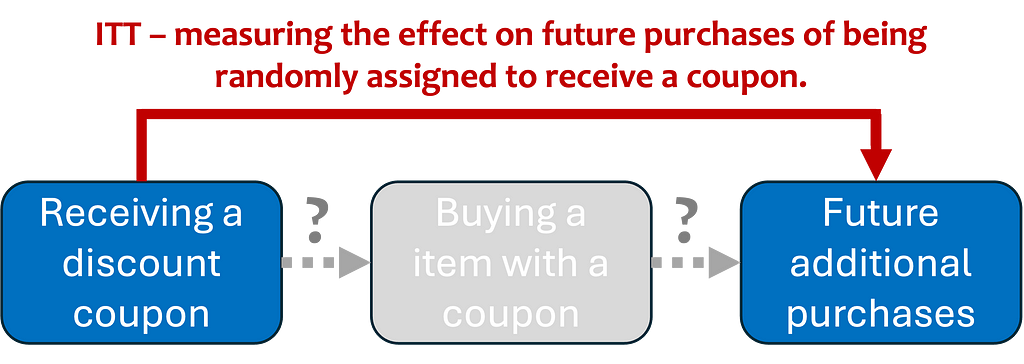
It measures the effect of being assigned to a treatment, regardless of whether individuals actually follow through with it. In our example, it compares the future average purchases of customers assigned to receive a coupon (treatment group) with those who were not (control group). This method is useful for understanding the effect of the assignment itself, but it may underestimate the treatment’s impact, as it includes individuals who did not use the coupon.

Local average treatment effect (LATE)

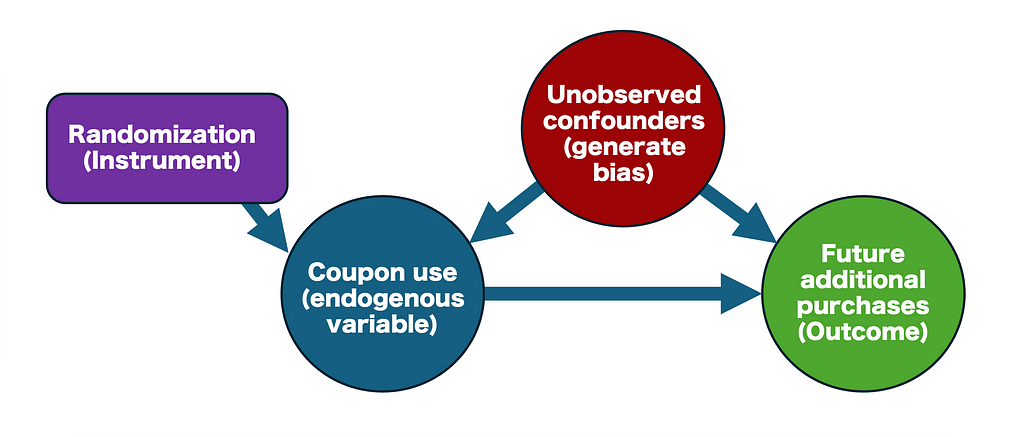
Here we use the instrumental variables (IV) method to estimate the local average treatment effect, which is the causal effect of treatment among those who complied with the assignment (“compliers”) — i.e., those who used the coupon because they were assigned to receive it. In summary:

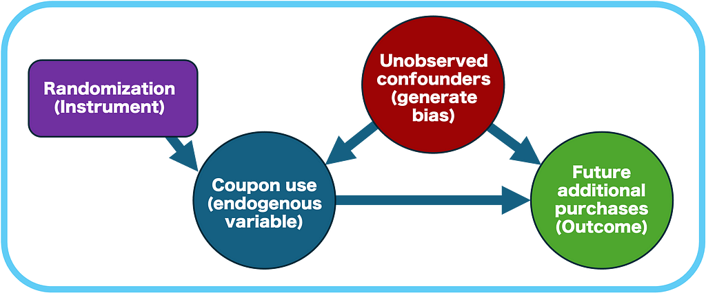
• The random assignment to treatment (receiving a coupon) is used as an instrumental variable that strongly predicts actual treatment uptake (using the coupon).
• The IV must meet specific assumptions (relevance, exogeneity, and exclusion restriction) that we will discuss in detail.
• The IV isolates the part of variation in coupon use that’s attributable to random assignment, eliminating the influence of unobserved factors that could bias the estimate (see more on “selection bias” here).
• The LATE estimates the effect of treatment by adjusting the impact of treatment assignment (ITT) for the compliance rate (the probability of using the coupon given that the customer was assigned).
• It is estimated via two-stage least squares (2SLS), in which each stage is illustrated in the figure below. An intuitive explanation of this method is discussed in section 5 here.

Assumptions and limitations

While the ITT estimate can be obtained directly by using OLS , IV methods require strong assumptions to provide valid causal estimates. Fortunately, those assumptions tend to be met in the experimental scenario:

Instrument relevance

The instrumental variable (in this case, assignment to the treatment group) must be correlated with the endogenous variable whose effect on future purchases we want to measure (coupon usage). In other words, random assignment to receive a coupon should significantly increase the likelihood that a customer uses it. This is tested via the magnitude and statistical significance of the treatment assignment coefficient in the first stage regression.

Instrument exogeneity and exclusion restriction

The instrumental variable must be independent of any unobserved factors that influence the outcome (future purchases). It should impact the outcome only through its effect on the endogenous variable (coupon usage).

In simpler terms, the instrument should influence the outcome only by affecting coupon usage, and not through any other pathway.

In our scenario, the random assignment of coupons ensures that it is not correlated with any unobserved customer characteristics that could affect future purchases. Randomization also implies that the impact of being assigned a coupon will primarily depend on whether the customer chooses to use it or not.

Limitations and challenges

1. The LATE provides the causal effect only for “compliers” — customers who used the coupon because they received it, and this effect is specific to this group (local validity only). It cannot be generalized to all customers or those who used the coupon for other reasons.
2. When compliance rates are low (meaning only a small proportion of customers respond to the treatment), the estimated effect becomes less precise, and the findings are less reliable. Since the effect is based on a small number of compliers, it is also difficult to determine if the results are meaningful for the broader population.
3. The assumptions of exogeneity and exclusion restriction are not directly testable, meaning that we must rely on the experimental design or on theoretical arguments to support the validity of the IV implementation.

Hands-on with instrumental variables using R

Now that we understand the intuition and assumptions, we will apply these techniques in an example to estimate both ITT and LATE in R. We will explore the following scenario, reproduced in this R script:

An e-commerce company wants to assess whether the use of discount coupons increases future customer purchases. To circumvent selection bias, coupons were randomly sent to a group of customers, but not all recipients used them. Additionally, customers who did not receive a coupon had no access to it.

I simulated a dataset representing that situation:

• treatment: Half of the customers were randomly assigned to receive the coupon (treatment = 1) while the other half did not receive (treatment = 0).
• coupon_use: Among the individuals who received treatment, those who used the coupon to make a purchase are identified by coupon_use = 1.
• income and age: simulated covariates that follow a normal distribution.
• prob_coupon_use: To make this more realistic, the probability of coupon usage varies among those who received the coupons. Individuals with higher income and lower age tend to have a higher likelihood of using the coupons.
• future_purchases: The outcome, future purchases in R$, is also influenced by income and age.
• past_purchases: Purchases in R$ from previous months, before the coupon assignment. This should not be correlated with receiving or using a coupon after we control for the covariates.
• Finally, the simulated effect of coupon usage for customers who used the coupon is set to “true_effect <- 50“. This means that, on average, using the coupon increases future purchases by R$50 for those who redeemed it.

Verifying Assumptions

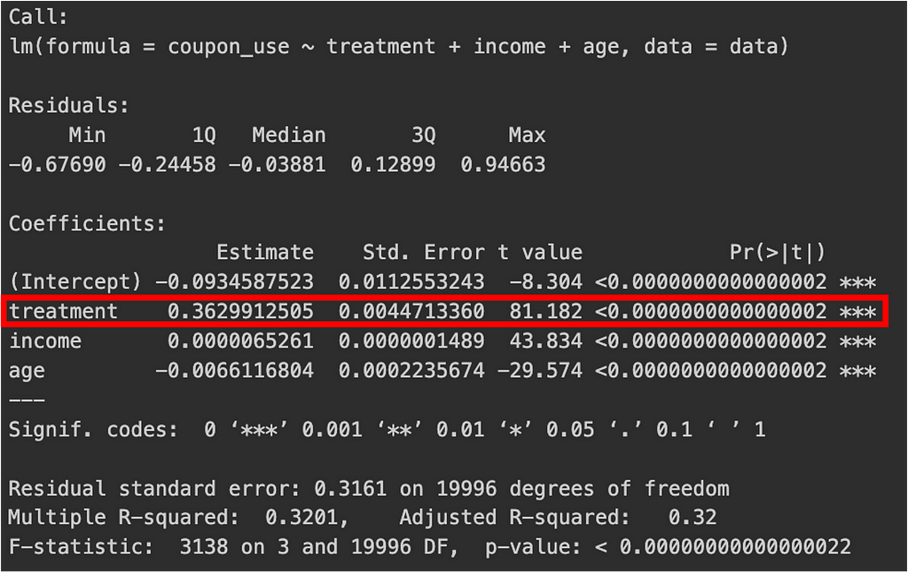
Instrument relevance: The first stage regression explains the relationship between belonging to the treatment group and the usage of the coupon. In this regression, the coefficient for “treatment” was 0.362, meaning that ~36% of the treatment group used the coupon. The p-value for this coefficient was < 0.01, with a t-statistic of 81.2 (substantial), indicating that treatment assignment (receiving a coupon) significantly influences coupon use.

Instrument exogeneity and exclusion restriction: By construction, since assignment is random, the instrument is not correlated with unobserved factors that affect future purchases. But in any case, these assumptions are indirectly testable via the two sets of results below:

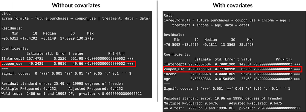
The first set includes regression results from the first (only in the script) and second stages (below), with and without covariates. These should yield similar results to support the idea that our instrument (coupon assignment) affects the outcome (future purchases) only through the endogenous variable (coupon use). Without covariates, the estimated effect was 49.24 with a p-value < 0.01, and with covariates, it was 49.31 with a p-value < 0.01.

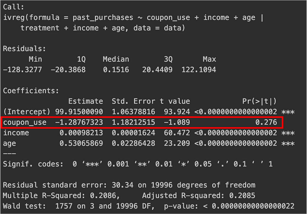
The second set involved a placebo test to determine whether the instrument affects past purchases (which it logically shouldn’t). This test suggests that the instrument does not have a direct effect on the outcome outside of its effect through the endogenous variable. The estimated effect, with or without covariates, was close to zero and not statistically significant.

LATE with two-stage least squares (2SLS)

Due to the nature of the indirect tests discussed above, we ended up anticipating the results of our main analysis, including the LATE (see the second figure of the subsection “Verifying Assumptions”). But now let’s go into more detail about this estimation process, which involves two steps using the 2SLS method:

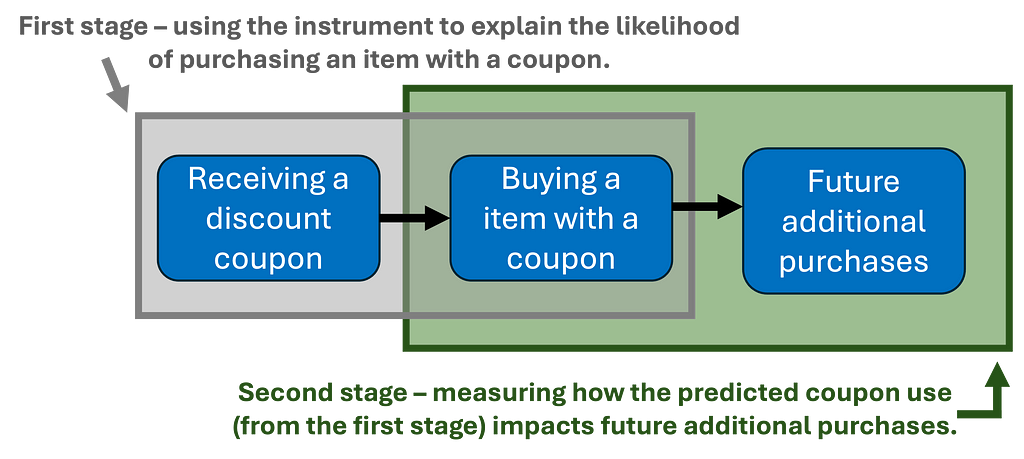
1. First stage: We regress coupon usage on treatment assignment. This generates predicted values of coupon usage, isolating the portion attributable to random assignment.
2. Second stage: We take the predicted coupon usage from the first stage and regress it against future purchases. This step allows us to estimate the causal impact of coupon usage.

first_stage <- lm(coupon_use ~ treatment + income + age, data = data)
second_stage <- ivreg(future_purchases ~ coupon_use + income + age | treatment + income + age, data = data)

By applying the 2SLS method, we derive an unbiased estimate of the causal effect of coupon usage specifically for those who comply with the treatment, effectively filtering out the influence of random assignment.

Estimating causal effects

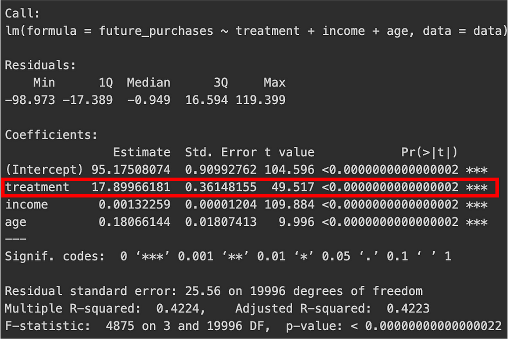
ITT estimate: It measures the average effect that offering a coupon has on customers’ future purchases. In our specific example, the coefficient for treatment was R$17.89 with a p-value < 0.01, while controlling for age and income. This indicates a significant effect of offering the coupon, although due to non-compliance, ITT will generally be lower than the true causal effect.

LATE estimate using IV: It represents the causal effect of coupon usage on future purchases among compliers (those who used the coupon because they received it). In our example, the estimated LATE was close to $50 (see the second figure in subsection “Verifying assumptions”), indicating that customers who complied by using the coupon saw their future purchases increase by roughly $50 compared to what would have happened without the coupon.

This result is larger than the ITT effect of R$17.89, as LATE focuses specifically on compliers, who are more likely to experience the true causal impact of using the coupon. Now you see how measuring LATE is important in experiments like this, helping us derive a more accurate understanding of the impact on individuals who actually use the treatment, and providing insights into the true efficacy of the intervention.

Just out of curiosity, run the following part of the script to learn that neither the difference in means between compliers and non-compliers, nor the difference between compliers and the control group, gives us the LATE simulated in the data — a point that many data professionals tend to overlook.

mean_compliers - mean_non_compliers # difference in means between compliers and non-compliers
mean_compliers - mean_control # difference in means between compliers and control

Insights to take home

Many data professionals focus only on the ITT estimate, often because it’s easier to explain or because they aren’t familiar with other estimands. However, the ITT effect can obscure the true impact on those who actually “consumed” the treatment. The LATE, on the other hand, provides a more accurate measure of the interventions effectiveness among compliers, offering insights that ITT alone cannot capture.

Although the instrumental variables (IV) approach may initially seem complex, random assignment in an experimental setup makes IV a powerful and reliable tool for isolating causal effects. Notice, however, that IV methods can also be applied beyond experimental contexts, provided the assumptions hold. For example, in a fuzzy regression discontinuity design (RDD), IV is a credible way to estimate local treatment effects, even though sharp RDD might appear more straightforward.

Thank you for reading. Follow me for more in this series 🙂

If you enjoyed this content and want to learn more about causal inference and econometrics, follow me here and on Linkedin, where I post about causal inference and career.

Would you like to support, me? Just share this with those who may be interested!

Recommended references

• Facure M. (2022). Causal Inference for the Brave and True, chapter 8 and chapter 9.
• Huntington-Klein N. (2021). The Effect: An Introduction to Research Design and Causality, chapter 19.

---

ITT vs LATE: Estimating Causal Effects with IV in Experiments with Imperfect Compliance was originally published in Towards Data Science on Medium, where people are continuing the conversation by highlighting and responding to this story.

In this post, we collaborate with the team working on PyTorch at Meta to showcase how the torchtitan library accelerates and simplifies the pre-training of Meta Llama 3-like model architectures. We showcase the key features and capabilities of torchtitan such as FSDP2, torch.compile integration, and FP8 support that optimize the training efficiency.

On multi-modal LLM Flamingo’s vision encoder

Designing Multi-modal LLM is hard.

The state-of-the-art multi-modal LLMs are primarily based on existing LLM architectures, with modifications specifically addressing different sources of input, and that’s where the difficulty comes from. The latest Nvidia paper divides the commonly used multi-modal architectures into two categories:

• decoder-based;
• cross-attention-based.

One of my previous medium articles discussed the latest paper from Meta, using decoder-based architecture, which converts an input image into a latent vector using a VAE encoder to address the issue that the image space is continuous and different from the discrete text space.

However, the problem with cross-attention-based architecture is different. For example, in the multi-modal LLM model Flamingo, the critical issue is converting the vision embedding from a generic vision model of varying temporal and spatial dimensions into the cross-attention layer to match the language input dimension.

In this post, I will dive deep into Flamingo’s unique design on top of the vision encoder, the Perceiver Resampler, to explain how this issue was solved. Furthermore, I will explore the Perceiver Resampler’s origin — the Induced Set Attention Block from Set Transformer, which further inspired DeepMind’s Perceiver model for learning fixed-length latent embeddings from generic input data.

Set Transformer

Published in 2019, the Set Transformer work extended the original Transformer model on sets to solve permutation-invariant problems like Set Anomaly Detection, Point Cloud Classification, etc. Inspired by the sparse Gaussian process where a small set of inducing variables could adequately approximate the posterior of an input, the Set Transformer uses the Induced Set Attention Blocks (ISAB) defined below:

MAB(X, Y) is the transformers’ original multi-head attention block, where query = X, key/value = Y. The ISAB block is almost identical to two stacked multi-head attention blocks, except that the input key/value is replaced by the inducing matrix I. The original set X is of dimension N*D, and I is of dimension M*D, representing M 1*D inducing points. A visualization is shown below.

Note that the design of the ISAB is to save computational cost. The reason is that the M could be much smaller than the original N dimension, which makes the time complexity of ISAB O(N*d) much smaller than the original self-attention complexity O(N**2*d).

Perceiver

Inspired by the use of inducing points as query matrix from Set Transformer, the Perceiver model, proposed by DeepMind, separated the query matrix as a short sequence of learnable latent embeddings (e.g., N=512) while the key and value pair to be a byte array that is an ultra-long sequence input (e.g., M=224*224 pixels).

The cross attention is borrowed from the decoder part of the original transformer, where the query and key/value come from different sources, and in this case, unlearnable representations:

Since K and V are input “constants,” the Perceiver transformer layer computational complexity becomes only relative to the latent space, which is O(N**2), and is also called a latent transformer. Decoupled from the input size, the latent transformers could quickly scale up to 48 layers, which is a great advantage over traditional transformer designs.

Flamingo’s Vision Encoder and Perceiver Resampler

Instead of applying the Perceiver directly, Flamingo first uses a pre-trained, CNN-based, weight-frozen Normalizer-Free ResNet (NFNet) to extract image/video features, then adds a learnable temporal positional embedding and flattens them to the 1D sequence. The Perceiver Resampler is attached to the vision encoder to learn a fixed-size latent embedding before being passed into the cross-attention layer of the leading architecture.

Like DeepMind’s Preceiver model, the Percerver Resampler uses constant input embeddings as keys/values and the learnable latent vectors as queries. Note that no spatial encoding is used here, and the rationale is that the previous vision encoder, NFNet, is a convolution-based model with spatial information embedded in the channel information. To increase performance, the learnable vectors are concatenated to the key/value vectors in the cross-attention computation.

The detailed algorithm is given below:

Summary

This article gives a detailed walk-through of the vision encoder part of the Flamingo architecture. The vision encoder has a unique design, the Perceiver Resampler, which originated from the Set Transformer and the Perceiver model and could minimize the cross-attention computation cost while leveraging information from both the spatial and temporal domains.

References

• Dai et al., NVLM: Open Frontier-Class Multimodal LLMs. arXiv 2024.
• Zhou et al., Transfusion: Predict the Next Token and Diffuse Images with One Multi-Modal Model. arXiv 2024.
• Alayrac et al., Flamingo: a Visual Language Model for Few-Shot Learning. NeurIPS 2022.
• Jaegle et al., Perceiver: General Perception with Iterative Attention. ICML 2021.
• Brock at al., High-Performance Large-Scale Image Recognition Without Normalization. arXiv 2021.
• Lee et al., Set Transformer: A Framework for Attention-based Permutation-Invariant Neural Networks. ICML 2019. Slides
• Vaswani et al., Attention Is All You Need. NeurIPS 2017.
• Stanford CS25: V1 I DeepMind’s Perceiver and Perceiver IO: new data family architecture, https://www.youtube.com/watch?v=wTZ3o36lXoQ
• HuggingFace, Perceiver Model Doc. https://huggingface.co/docs/transformers/v4.34.0/en/model_doc/perceiver

---

From Set Transformer to Perceiver Sampler was originally published in Towards Data Science on Medium, where people are continuing the conversation by highlighting and responding to this story.

7 steps that helped me transition from a software engineer to machine learning engineer

I receive a lot of inquiries (a LOT) about how to transition from a software engineer to a machine learning engineer (MLE) at FAANG companies. Having successfully transitioned myself, I can say that the biggest challenge I faced was not knowing where to start and feeling lost without a clear plan.

In this article, I am sharing the step-by-step approach that will help you navigate this change. These 7 steps helped me transition from a software engineer to Machine Learning engineer.

Let’s dive in.

1. Motivation

Find out why

Why Machine Learning? Machine Learning and AI are super hot right now, but you should understand why you want to get into it. This personal motivation will keep you going even when the AI hype dies down.

What Got Me Hooked: For me, it was about how Google search was developed. The way Google could find exactly what I needed so quickly really made me want to know more about the tech behind it. That curiosity got me into Learning to Rank algorithms starting with PageRank and then broader machine learning.

Questions to Ask Yourself:

• What part of Machine Learning really grabs my interest? Is it the hot trend or something else?
• Are there any specific ML applications I like? For me it is Natural Language Processing and Recommendations, but maybe you’re into using ML in FinTech.

Take Your Time to Explore

It took me 4 years (1 year in Masters, 1 year in PhD where I dropped out, and 2 years in the industry) to realize what I really wanted to do. This is ok. It takes time to build experience and know enough about a new field which is as big as ML.

• Build the Basics: Start with the fundamentals like statistics and machine learning basics. This solid base will help you get a better grasp of the field and find the area you’re most excited about.
• Networking and Mentorship: Chat with people who are already in the field, find some mentors working around you, and get a feel of their day-to-day work to see if it excites you.
• Understand Your Options: Find out what kind of ML role interests you, whether that’s being an Applied ML Engineer, ML Researcher, or working in MLOps. Learn about different roles in one of my previous article here.

2. Find Your Niche

Understanding your motivations and interests will naturally lead you to identify where you can best apply your skills within the ML landscape.

• Be Strategic: Often ML roles will have certain required qualifications like 5 years of relevant industry experience or PhD. If your experience does not match with the required qualifications, it may not be the right fit at that time. Focus on building your skills step by step and find roles strategically that aligns more with your current experience.
• Find the Sweet Spot: If possible, use your current domain knowledge to your advantage. Transitioning within a domain you’re already familiar with is easier. As a software engineer, you are already aware of critical metrics, business goals and domain specific problems. Identify where you can contribute the most, take ownership, and aim to lead in that area.

I started working as a software engineer in the Amazon Pricing team. Even though Pricing as a domain was not my preferred choice, but due to extensive amount of experience I acquired there, it helped me to transition to MLE much faster.

3. Be open to compromises

In your career, you’ll sometimes face decisions that require short-term sacrifices for long-term gains, especially when entering a new field. Here are some tough choices I had to make during my switch:

• Rejected my dream company Google’s offer twice: I received offer letters from Google, which offered a higher salary, but I turned them down because the role involved Android development, which had no ML opportunities. Instead, I chose Amazon, where the role didn’t initially involve ML either but allowed me to work more closely with ML teams. To date, the best choice I have made in my life!!

• Delayed my promotion for almost 3 years: I had the chance to be promoted to senior software engineer at Amazon much sooner. A senior software engineer transition to a senior MLE is much harder due to increased expectations. Knowing this, I chose to delay my promotion to keep my options open.

4. Find a supportive manager / company

If you’ve pinned down a domain you’re passionate about, you’ll still need a supportive manager and company to make the transition successfully.

Find the Right Environment:

• Look for ML Opportunities: Seek out teams within your company that offer the chance to work on ML projects. Join a team that has both software engineering and ML teams working closely, luckily most teams are like that. If your current company lacks these opportunities, consider looking outside.

Tip: Find teams that has transitioned Software Engineers to MLEs in the past. This can greatly accelerate your transition as these teams often have a clear guideline for the transition.

• Find a Supportive Manager: A manager familiar with ML roles and who is supportive of your learning and career growth is crucial. They should not only support you verbally but also take active steps to facilitate your transition.

Tip: Always draft a document outlining your transition plan and the projects you’d like to work on and discuss in your 1:1s with your manager. If they repeatedly show disinterest, they might not be motivated to help you switch roles.

5. Gain trust by being a reliable software engineer

In my first team at Amazon, I gave my 200% as a software engineer, even though the role wasn’t my ideal choice. My goal was to make myself indispensable, allowing me to choose the projects I wanted to work on. This effort built a trusting relationship with my manager, where we valued each other’s advice.

Why is this important? Typically, only top engineers get to choose their projects, while others must tackle the tasks assigned to them. Demonstrating reliability can give you opportunities that might otherwise be unattainable and give you more control over your career path.

6. Work on projects

Once you’ve joined a team with ML opportunities, a supportive manager, and relevant domain space, it’s time to apply your foundational knowledge.

Work on small projects on the side:

• Collaborate with experienced ML engineers to work on small features for model training or minor model changes. These tasks might fall outside your primary job responsibilities.

For instance, I worked on a project to improve the AWS SageMaker training pipeline in my team at Amazon. This allowed me to work more closely with ML engineers in the team, understand their development process and contribute to development of new features in upcoming model iterations.

Expand Your Scope:

• As you gain confidence in the problem space, begin to explore the broader domain. Research extensively to understand the challenges and limitations of current system and identify potential areas for improvement.

Tip: Read blogs and research articles from other companies within the same space to understand challenges faced by companies to get potential ideas for improvement. For example when I was at Amazon, I followed tech articles from other eCommerce platforms like eBay and Walmart.

• This is your opportunity to think creatively and identify original solutions. Maintain a detailed document to track all your learnings throughout this. Include design documents, technical insights, practical challenges, solutions you’ve implemented, and any feedback or evaluations you receive. Not only is it a valuable learning tool to keep track of your learning, but it also acts as tangible evidence during your transition evaluation.

7. Understand Performance Evaluation

Transitions like promotions are lagging indicators, meaning that any new role requires the individual to already be performing at the level expected for that role. Identify the criteria that will be used for evaluation during your transition to an MLE role. Generally, Software Engineers and MLEs are evaluated differently during performance feedback sessions.

With Software Engineer, often the emphasis is more on scalable system design, code quality and project complexity. With MLE, generally the emphasis is much more on Impact to the business metric and technical expertise. This is because, ML has a longer cycle of development compared to software engineering and are often directly tied to specific business metrics.

Parting Note

The Software Engineer to MLE transition can be as challenging as it is rewarding. It requires a blend of strategic planning, continuous learning, and adaptability.

Few more bonus tips:

• Find a Mentor: Seek out a mentor within the team where you are making the transition. This mentor will support you throughout your transition process, help resolve any blockers, and identify new opportunities for you.
• Track Your Learnings: Maintain a detailed record of all your learnings throughout your transition. This documentation will allow you to revisit and refine ideas and also act as a reference during performance evaluations.
• Communicate Proactively: Regularly communicate with your team and manager about both the challenges you encounter and the successes you achieve. Open communication will help in adjusting strategies as needed and ensure continued support from your team.

These strategies have been instrumental in navigating my career transition effectively. By following above steps, you can improve your journey and set a solid foundation for success in your new role as a Machine Learning Engineer.

Best of luck and as always Happy Learning!

If this article was helpful to you and you want to learn more about real-world tips for Machine Learning, Sign up for my newsletter or connect with me on LinkedIn.

Disclaimer: This blog is based on personal experiences and publicly available resources. Please note, the opinions expressed are solely my own and do not represent those of my past or current employers. Always refer to official resources and guidelines from hiring companies for the most accurate information.

---

Make the Switch from Software Engineer to ML Engineer was originally published in Towards Data Science on Medium, where people are continuing the conversation by highlighting and responding to this story.

A brief tour of how caching works in attention-based models

I’ve been exploring articles about how Prompt Caching works, and while a few blogs touch on its usefulness and how to implement it, I haven’t found much on the actual mechanics or the intuition behind it.

The question really comes down to this: GPT-like model generation relies on the relationships between every token in a prompt. How could caching just part of a prompt even make sense?

Surprisingly, it does. Let’s dive in!

Prompt caching has recently emerged as a significant advancement in reducing computational overhead, latency, and cost, especially for applications that frequently reuse prompt segments.

To clarify, these are cases where you have a long, static pre-prompt (context) and keep adding new user questions to it. Each time the API model is called, it needs to completely re-process the entire prompt.

Google was the first to introduce Context Caching with the Gemini model, while Anthropic and OpenAI have recently integrated their prompt caching capabilities, claiming great cost and latency reduction for long prompts.

What is Prompt Caching?

Prompt caching is a technique that stores parts of a prompt (such as system messages, documents, or template text) to be efficiently reused. This avoids reprocessing the same prompt structure repeatedly, improving efficiency.

There are multiple ways to implement Prompt Caching, so the techniques can vary by provider, but we’ll try to abstract the concept out of two popular approaches:

• GPTCache: Semantic Cache for LLMs
• Prompt Cache: Modular Attention Reuse

The overall process goes as follows:

1. When a prompt comes in, it goes through tokenization, vectorization, and full model inference (typically an attention model for LLMs).
2. The system stores the relevant data (tokens and their embeddings) in a cache layer outside the model. The numerical vector representation of tokens is stored in memory.
3. On the next call, the system checks if a part of the new prompt is already stored in the cache (e.g., based on embedding similarity).
4. Upon a cache hit, the cached portion is retrieved, skipping both tokenization and full model inference.

So… What Exactly is Cached?

In its most basic form, different levels of caching can be applied depending on the approach, ranging from simple to more complex. This can include storing tokens, token embeddings, or even internal states to avoid reprocessing:

• Tokens: The next level involves caching the tokenized representation of the prompt, avoiding the need to re-tokenize repeated inputs.
• Token Encodings: Caching these allows the model to skip re-encoding previously seen inputs and only process the new parts of the prompt.
• Internal States: At the most complex level, caching internal states such as key-value pairs (see below) stores relationships between tokens, so the model only computes new relationships.

Caching Key-Value States

In transformer models, tokens are processed in pairs: Keys and Values.

• Keys help the model decide how much importance or “attention” each token should give to other tokens.
• Values represent the actual content or meaning that the token contributes in context.

For example, in the sentence “Harry Potter is a wizard, and his friend is Ron,” the Key for “Harry” is a vector with relationships with each one of the other words in the sentence:

[“Harry”, “Potter”], [“Harry””, “a”], [“Harry”, “wizard”], etc…

How KV Prompt Caching Works

1. Precompute and Cache KV States: The model computes and stores KV pairs for frequently used prompts, allowing it to skip re-computation and retrieve these pairs from the cache for efficiency.
2. Merging Cached and New Context: In new prompts, the model retrieves cached KV pairs for previously used sentences while computing new KV pairs for any new sentences.
3. Cross-Sentence KV Computation: The model computes new KV pairs that link cached tokens from one sentence to new tokens in another, enabling a holistic understanding of their relationships.

In summary:

All of the relationships between tokens of the cached prompt are already computed. Only new relationships between NEW-OLD or NEW-NEW tokens must be computed.

Is This the End of RAG?

As models’ context sizes increase, prompt caching will make a great difference by avoiding repetitive processing. As a result, some might lean toward just using huge prompts and skipping retrieval processes entirely.

But here’s the catch: as contexts grow, models lose focus. Not because models will do a bad job but because finding answers in a big chunk of data is a subjective task that depends on the use case needs.

Systems capable of storing and managing vast volumes of vectors will remain essential, and RAG goes beyond caching prompts by offering something critical: control.

With RAG, you can filter and retrieve only the most relevant chunks from your data rather than relying on the model to process everything. A modular, separated approach ensures less noise, giving you more transparency and precision than full context feeding.

Finally, larger context models emerging will probably ask for better storage for prompt vectors instead of simple caching. Does that take us back to… vector stores?

At Langflow, we’re building the fastest path from RAG prototyping to production. It’s open-source and features a free cloud service! Check it out at https://github.com/langflow-ai/langflow ✨

---

Prompt Caching in LLMs: Intuition was originally published in Towards Data Science on Medium, where people are continuing the conversation by highlighting and responding to this story.

In this blog post, we explore a comprehensive approach to time series forecasting using the Amazon SageMaker AutoMLV2 Software Development Kit (SDK). SageMaker AutoMLV2 is part of the SageMaker Autopilot suite, which automates the end-to-end machine learning workflow from data preparation to model deployment.