In this post, we dive into the Rufus inference deployment using AWS chips and how this enabled one of the most demanding events of the year—Amazon Prime Day.
In this post we discuss how you can maintain access to Lookout for Vision after it is closed to new customers, some alternatives to Lookout for Vision, and how you can export your data from Lookout for Vision to migrate to an alternate solution.
Agents have rapidly emerged in recent months as one of the most promising modalities for harnessing the power of AI to perform day-to-day tasks. Their growing popularity comes with a nontrivial amount of confusion, though—from what they actually are (the anthropomorphic term itself doesn’t help in that regard) to how and in what contexts they can be used effectively.
This week, we’ve put together a strong lineup of recent articles that will help beginners and experienced practitioners alike to find their bearings around this topic and to make informed decisions about adopting agents in their own workflows. From their core traits to broader questions on reasoning and alignment, these posts cover agents from a technical and practical perspective, while placing them in the context of AI’s growing footprint in our daily lives. Let’s dive in!
What Makes a True AI Agent? Rethinking the Pursuit of Autonomy “Even if we could build fully autonomous AI agents, how often would they be the best thing for users?” Julia Winn explores the fundamental traits of agents, adds much-needed nuance to our understanding of what they are—and what they aren’t, and proposes a spectrum of agentic behavior as a framework to assess their suitability for specific tasks.
Exploring the AI Alignment Problem with Gridworlds Where do agents fit within the ongoing debates surrounding AI safety? What does it take to ensure the outcomes they produce are aligned with their creators’ goals? Tarik Dzekman opens up a thoughtful conversation on a thorny topic: “how hard it is to build a AI agents capable of solving a problem without also encouraging it to make make decisions that we wouldn’t like.”
AI Agents: The Intersection of Tool Calling and Reasoning in Generative AI One of the main benefits of AI agents is their ability to bridge the gaps between disparate tools and workflows in a streamlined, automated, and (ideally) predictable way. Tula Masterman’s lucid overview focuses on how reasoning is expressed through tool calling, explores some of the challenges agents face with tool use, and covers common ways to evaluate their tool-calling ability.
The AI Developer’s Dilemma: Proprietary AI vs. Open Source Ecosystem If you’re in the process of implementing agents (and other AI-powered solutions) in your projects, one of the key questions you’ll have to answer sooner rather than later is whether to rely on proprietary or open-source products to get you there. Gadi Singer shares a detailed breakdown of the advantages and limitations of each approach.
For other excellent articles on topics ranging from geospatial data to the complex art of scoring professional tango dancers, don’t miss this week’s recommended reads:
Thank you for supporting the work of our authors! As we mentioned above, we love publishing articles from new authors, so if you’ve recently written an interesting project walkthrough, tutorial, or theoretical reflection on any of our core topics, don’t hesitate to share it with us.
Multi-modal LLM development has been advancing fast in recent years.
Although the commercial multi-modal models like GPT-4v, GPT-4o, Gemini, and Claude 3.5 Sonnet are the most eye-catching performers these days, the open-source models such as LLaVA, Llama 3-V, Qwen-VL have been steadily catching up in terms of performance on public benchmarks.
Just last month, Nvidia released their open-source multi-modal LLM family called NVLM. The family comprises three architectures: a) decoder-based, b) cross-attention-based, and c) hybrid. The decoder-based model takes both the image and text tokens to a pre-trained LLM, such as the LLaVA model. The cross-attention-based model uses the image token embeddings as the keys and values while using the text token embeddings as the queries; since the attention is calculated using different sources, it’s called “cross-attention” as in the original transformer decoder rather than the self-attention as in decoder-only models. The hybrid architecture is a unique design merging the decoder and cross-attention architecture for the benefit of multi-modal reasoning, fewer training parameters, and taking high-resolution input. The 72B decoder-based NVLM-D model achieved an impressive performance, beating state-of-the-art open-source and commercial models on tasks like natural image understanding and OCR.
In this article, I’m going to walk through the following things:
the dynamic high-resolution (DHR) vision encoder, which all the NVLM models adopt
the decoder-based model, NVLM-D, compared to LLaVA
the gated cross-attention model, NVLM-X, compared to Flamingo
the hybrid model, NVLM-H
In the end, I’ll show the NVLM-D 72B performance. Compared to state-of-the-art open-source and commercial models, the NVLM-D model shows stability over text-based tasks and superior performance on natural understanding and OCR tasks.
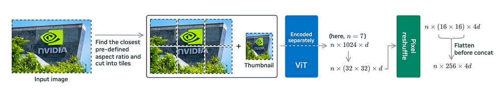
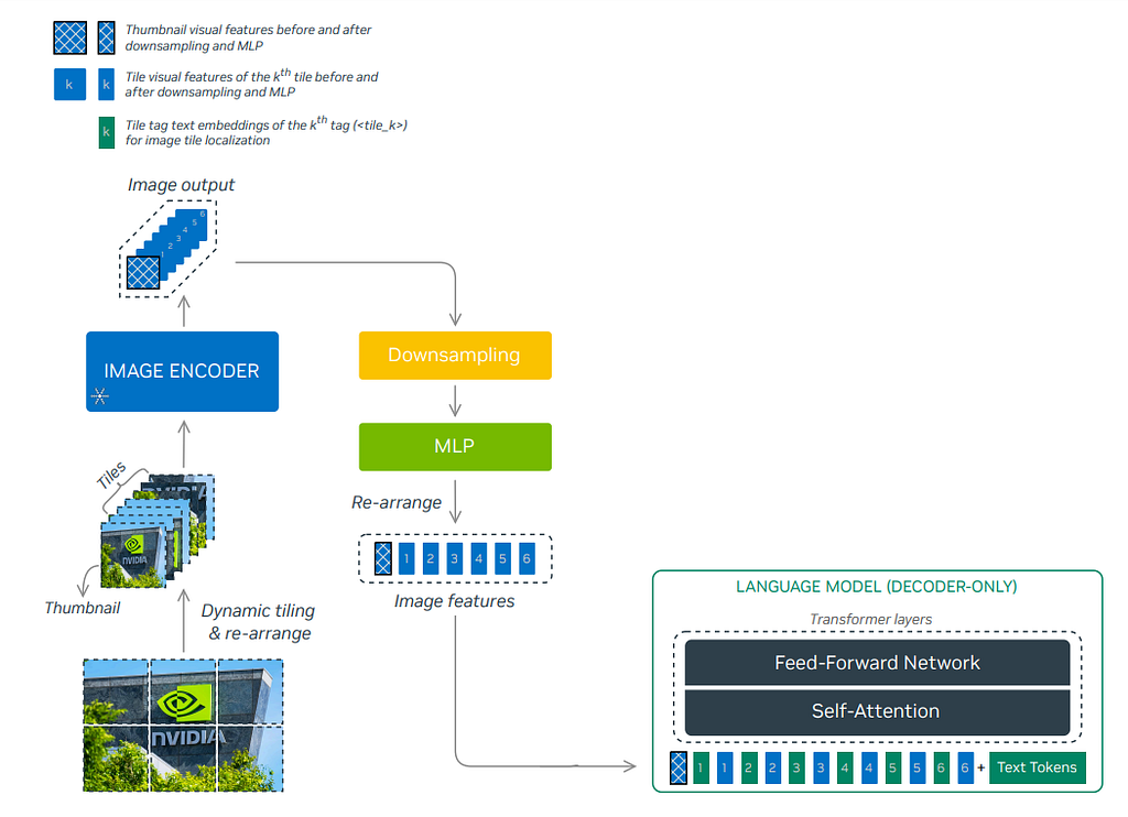
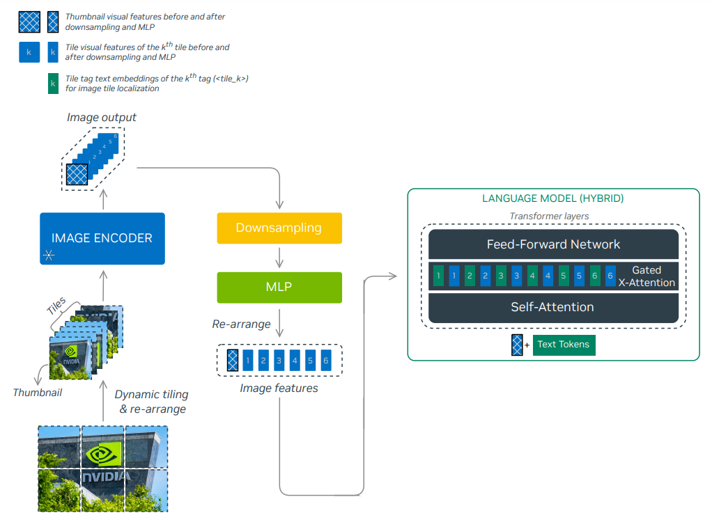
One of the prominent advantages of NVLM models is that they excel in processing OCR-related tasks, which require high-resolution image inputs. NVML adopts the dynamic high-resolution approach proposed in the InternVL 1.5technical report to retain high resolution. The DHR approach first converts a high resolution image into a pre-defined aspect ratio size (also called dynamic aspect ratio matching), before splitting it into non-overlapping 448*448 tiles with an extra thumb-nail image, which can retain better global information.
The image above shows a detailed explanation of the DHR pipeline. An input image is shown on the left, and a list of 6 different pre-defined aspect ratios is searched and matched to the original image shape. Then, the reshaped image is cropped into six non-overlapping tiles of 448*448, with an extra underresolution thumbnail image to capture global information. The sequence of n tiles (n=6+1=7 in this case) is passed into the ViT separately and converted into a sequence of length n with 1024 tokens (448/14*448/14=1024), each of embedding dimension d. To reduce the computational cost, a pixel reshuffle operation is employed to resize the 32*32 patch to 16*16, which reduces the final output token size to 256 with an increased embedding dimension of 4*d.
Decoder-only Models: NVLM-D vs LLaVA
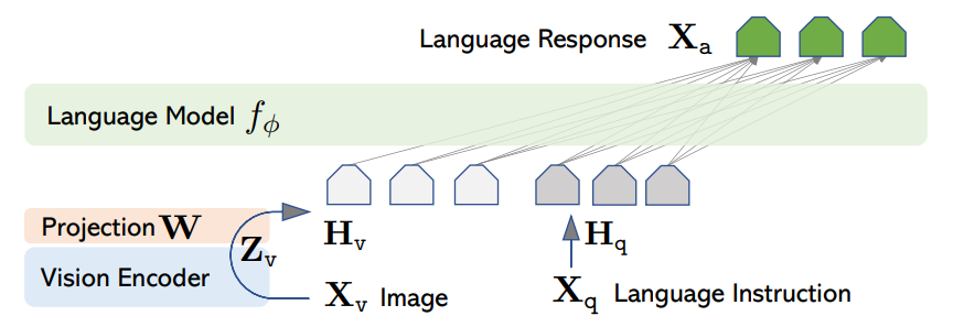
LLaVA is a well-known decoder-based Multi-modal LLM, which takes in the image X_v and uses a pre-trained CLIP encoder ViT-L/14 as vision encoder Z_v, with a trainable linear project layer W to convert into embedding tokens H_v, which can be digested together with other text tokens. The LLaVA architecture is shown below.
In contrast, the NVLM-D architecture takes in encoded tile sequence tokens using the DHR vision encoder and inserts tile tags in between before concatenating with the text tokens for the transformer layer ingestion. The architecture is shown below.
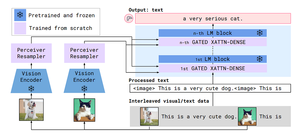
Comparing to LLaVA, the Flamingo model uses a more complicated cross-attention technique, which takes the vision embeddings as keys (K) and values (V), while the text embeddings as queries (Q). Moreover, the vision encoder is a CNN-based model with a Perceiver Resampler, which takes in a sequence of image(s) with temporal positional embedding to train learnable latent query vectors using cross attention. A more detailed discussion of the Perceiver Resampler can be found in my latest article here.
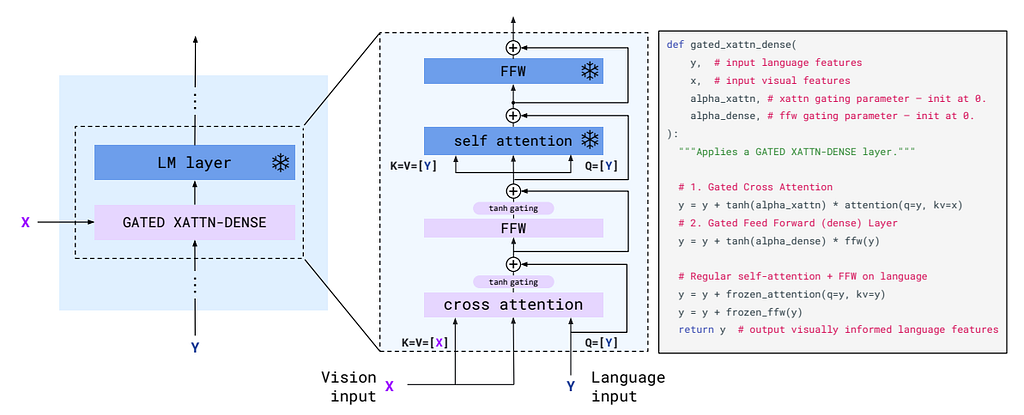
To fuse the vision embedding and text embedding, the Flamingo freezes the pre-trained LLM layers and further adds a trainable gated cross-attention layer in between, which is shown below. The gated attention uses a tanh gating with a learnable alpha parameter after the cross-attention layer and the subsequent linear layer. When the tanh gating is initialized as zero, the only information passed is through the skip connection, so the whole model will still be the original LLM to increase stability.
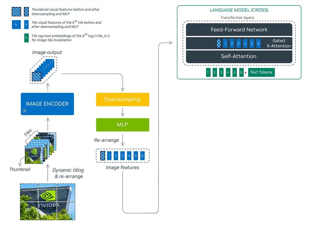
In comparison, the NVLM-X removes the Perceiver Resampler design for the benefit of OCR tasks to keep the more spatial relationship and only uses the DHR encoder output for the gated cross-attention. Unlike the decoder-based model, the NVLM-X concatenates the tile tags to the text tokens before sending them into the gated cross-attention. The whole architecture is shown below.
The hybrid model is a unique design by NVLM. The thumbnail image token is added to the text tokens as input to the self-attention layer, which preserves the benefit of multi-modal reasoning from the decoder-based model. The other image tiles and tile tags are passed into the gated cross-attention layer to capture finer image details while minimizing total model parameters. The detailed architecture is shown below.
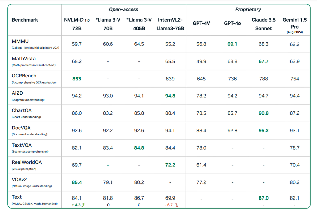
So, how’s the performance of NVLM compared to other state-of-the-art models? The paper lists benchmark performances comparing NVLM-D 72B to other open-source models like Llama-3 V and commercial models like GPT-4o. The NVLM-D achieved above-average performance on most benchmarks and excelled in the OCR and natural image understanding tasks due to the high-resolution image features and the model’s intrinsic multi-modal reasoning ability. Compared to Llama 3-V 70B and InternVL2-Llama3–76B, which have the equivalent amount of parameter numbers, the NVLM-D shows the advantage of having more consistent behaviours on the text-only tasks, the VQA task and the image understanding tasks. The detailed comparison is shown as follows.
NVLM-D performance compared to other open-source and commercial models on public benchmarks. Image source: https://arxiv.org/pdf/2409.11402
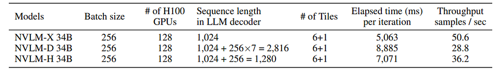
It’s also interesting to note that, although the decoder-based model is very powerful, the training throughput (numbers of sampled trained per second) is much lower than the cross-attention-based model. The paper explains that the decoder-based model takes a much longer sequence length than the cross-attention-based model, which causes a much higher GPU consumption and lower throughput. The detailed training comparison is shown below:
Azure Data Factory (ADF) is a popular tool for moving data at scale, particularly in Enterprise Data Lakes. It is commonly used to ingest and transform data, often starting by copying data from on-premises to Azure Storage. From there, data is moved through different zones following a medallion architecture. ADF is also essential for creating and restoring backups in case of disasters like data corruption, malware, or account deletion.
This implies that ADF is used to move large amounts of data, TBs and sometimes even PBs. It is thus important to optimize copy performance and so to limit throughput time. A common way to improve ADF performance is to parallelize copy activities. However, the parallelization shall happen where most of the data is and this can be challenging when the data lake is skewed.
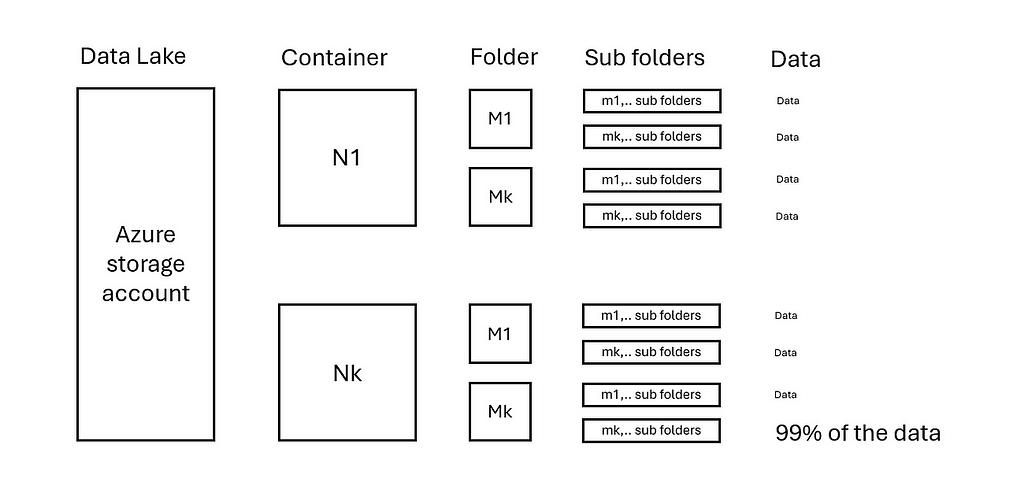
Data Lakes come in all sizes and manners. It is important to understand the data distribution within a data lake to improve copy performance. Consider the following situation:
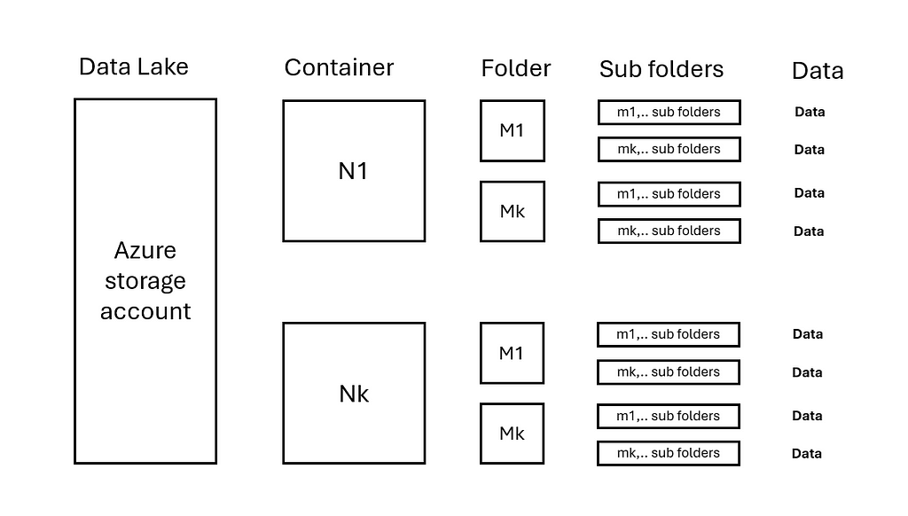
An Azure Storage account has N containers.
Each container contains M folders and m levels of sub folders.
Data is evenly distributed in folders N/M/..
See also image below:
2.1 Data lake with uniformly distributed data — image by author
In this situation, copy activities can be parallelized on each container N. For larger data volumes, performance can be further enhanced by parallelizing on folders M within container N. Subsequently, per copy activity it can be configured how much Data Integration Units (DIU) and copy parallelizationwithin a copy activity is used.
Now consider the following extreme situation that the last folder Nk and Mk has 99% of data, see image below:
2.2 Data lake with skewed distributed data — image by author
This implies that parallelization shall be done on the sub folders in Nk/Mk where the data is. More advanced logic is then needed to pinpoint the exact data locations. An Azure Function, integrated within ADF, can be used to achieve this. In the next chapter a project is deployed and are the parallelization options discussed in more detail.
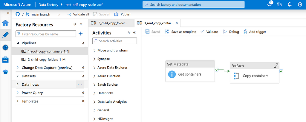
Run the script deploy_adf.ps1. In case ADF is successfully deployed, there are two pipelines deployed:
3.1.1 Data Factory project with root and child pipeline — image by author
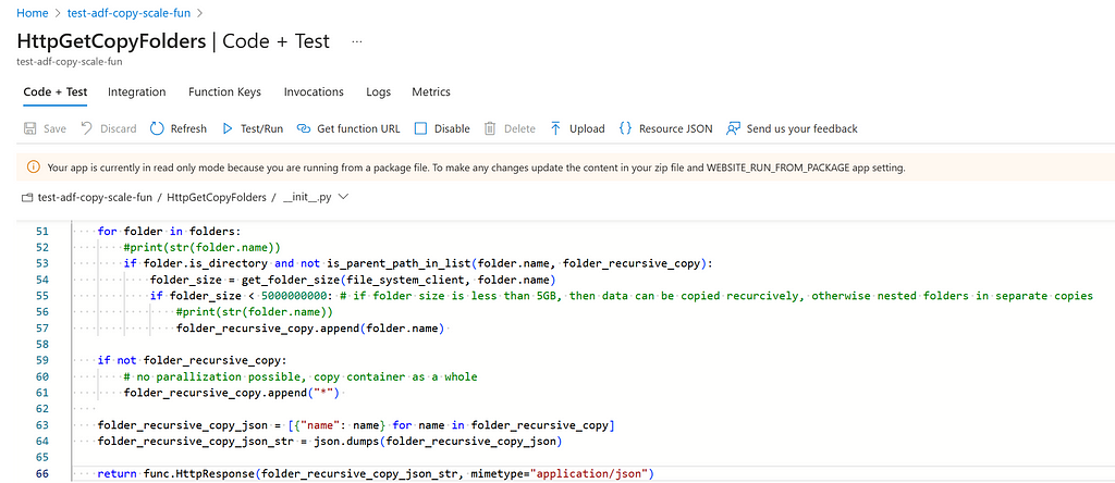
Subsequently, run the script deploy_azurefunction.ps1. In case the Azure Function is successfully deployed, the following code is deployed.
3.1.2 Azure Function to find “pockets of data” such that ADF can better parallelize
To finally run the project, make sure that the system assigned managed identity of the Azure Function and Data Factory can access the storage account where the data is copied from and to.
3.2 Parallelization used in project
After the project is deployed, it can be noticed that the following tooling is deployed to improve the performance using parallelization.
Root pipeline: Root pipeline that lists containers N on storage account and triggers child pipeline for each container.
Child pipeline: Child pipeline that lists folders M in a container and triggers recursive copy activity for each folder.
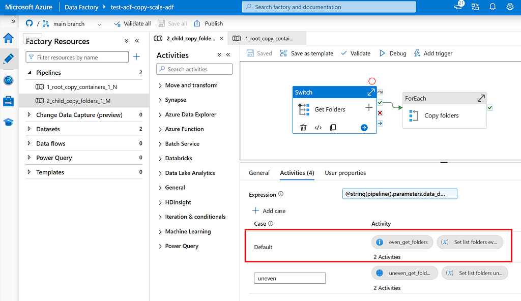
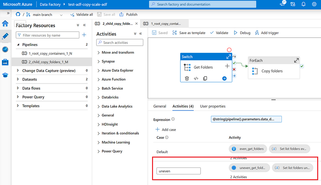
Switch: Child pipeline uses a switch to decide how list folders shall be determined. For case “default” (even), Get Metadata is used, for case “uneven” an Azure Function is used.
Get Metadata: List all root folders M in a given container N.
Azure Function: List all folders and sub folders that contain no more than X GB of data and shall be copied as a whole.
Copy activity: Recursively copy for all data from a given folder.
DIU: Number of Data Integration Units per copy activity.
Copy parallelization: Within a copy activity, number of parallel copy threads that can be started. Each thread can copy a file, maximum of 50 threads.
In the uniformly distributed data lake, data is evenly distributed over N containers and M folders. In this situation, copy activities can just be parallelized on each folder M. This can be done using a Get Meta Data to list folders M, For Each to iterate over folders and copy activity per folder. See also image below.
3.2.1 Child pipeline structure focusing on uniformly distributed data
Using this strategy, this would imply that each copy activity is going to copy an equal amount of data. A total of N*M copy activities will be run.
In the skewed distributed data lake, data is not evenly distributed over N containers and M folders. In this situation, copy activities shall be dynamically determined. This can be done using an Azure Function to list the data heavy folders, then a For Each to iterate over folders and copy activity per folder. See also image below.
3.2.2 Child pipeline structure focusing on skewed distributed data
Using this strategy, copy activities are dynamically scaled in data lake where data can be found and parallelization is thus needed most. Although this solution is more complex than the previous solution since it requires an Azure Function, it allows for copying skewed distributed data.
3.3: Parallelization performance test
To compare the performance of different parallelization options, a simple test is set up as follows:
Two storage accounts and 1 ADF instance using an Azure IR in region westeurope. Data is copied from source to target storage account.
Source storage account contains three containers with 0.72 TB of data each spread over multiple folders and sub folders.
Data is evenly distributed over containers, no skewed data.
Test A: Copy 1 container with 1 copy activity using 32 DIU and 16 threads in copy activity (both set to auto) => 0.72 TB of data is copied, 12m27s copy time, average throughput is 0.99 GB/s
Test B: Copy 1 container with 1 copy activity using 128 DIU and 32 threads in copy activity => 0.72 TB of data is copied, 06m19s copy time, average throughput is 1.95 GB/s.
Test C: Copy 1 container with 1 copy activity using 200 DIU and 50 threads (max) => test aborted due to throttling, no performance gain compared to test B.
Test D: Copy 2 containers with 2 copy activities in parallel using 128 DIU and 32 threads for each copy activity => 1.44 TB of data is copied, 07m00s copy time, average throughput is 3.53 GB/s.
Test E: Copy 3 containers with 3 copy activities in parallel using 128 DIU and 32 threads for each copy activity => 2.17 TB of data is copied, 08m07s copy time, average throughput is 4.56 GB/s. See also screenshot below.
3.3 Test E: Copy throughput of 3 parallel copy activities of 128 DIU and 32 threads, data size is 3*0.72TB
In this, it shall be noticed that ADF does not immediately start copying since there is a startup time. For an Azure IR this is ~10 seconds. This startup time is fixed and its impact on throughput can be neglected for large copies. Also, maximum ingress of a storage account is 60 Gbps (=7.5 GB/s). There cannot be scaled above this number, unless additional capacity is requested on the storage account.
The following takeaways can be drawn from the test:
Significant performance can already be gained by increasing DIU and parallel settings within copy activity.
By running copy pipelines in parallel, performance can be further increased.
In this test, data was uniformly distributed across two containers. If the data had been skewed, with all data from container 1 located in a sub folder of container 2, both copy activities would need to target container 2. This ensures similar performance to Test D.
If the data location is unknown beforehand or deeply nested, an Azure Function would be needed to identify the data pockets to make sure the copy activities run in the right place.
4. Conclusion
Azure Data Factory (ADF) is a popular tool to move data at scale. It is widely used for ingesting, transforming, backing up, and restoring data in Enterprise Data Lakes. Given its role in moving large volumes of data, optimizing copy performance is crucial to minimize throughput time.
In this blog post, we discussed the following parallelization strategies to enhance the performance of data copying to and from Azure Storage.
Within a copy activity, utilize standard Data Integration Units (DIU) and parallelization threads within a copy activity.
Run copy activities in parallel. If data is known to be evenly distributed, standard functionality in ADF can be used to parallelize copy activities across each container (N) and root folder (M).
Run copy activities where the data is. In case this is not known on beforehand or deeply nested, an Azure Function can be leveraged to locate the data. However, incorporating an Azure Function within an ADF pipeline adds complexity and should be avoided when not needed.
Unfortunately, there is no silver bullet solution and it always requires analyses and testing to find the best strategy to improve copy performance for Enterprise Data Lakes. This article aimed to give guidance in choosing the best strategy.
Coding the connectors yourself? Think very carefully
Creating and maintaining a data platform is a hard challenge. Not only do you have to make it scalable and useful, but every architectural decision builds up over time. Data connectors are an essential part of such a platform. Of course, how else are we going to get the data? And building them yourself from scratch gives you full control of how you want them to behave. But beware, with ever-increasing data sources in your platform, that can only mean the following:
Creating large volumes of code for every new connector.
Maintaining complex code for every single data connector.
Functions and definitions between classes may diverge over time, resulting in even more complex maintenance.
Of course, all three can be mitigated with well-defined practices in object-oriented programming. But even still, it will take many hours of coding that could be used in later stages to serve your data consumers faster.
Other options still give you the flexibility to define what data you want to ingest and how with no to very little code involved. With this option, you get:
Connectors with standardized behavior given the extraction methodology: No divergent classes for two connectors that use REST APIs at their core, for instance.
Simple, but powerful user interfaces to build connections between sources and destinations.
Connectors that are maintained by the teams building the tools and the community.
These benefits allow you to build data connections in minutes, instead of hours.
Nevertheless, I am not trying to sell you these tools; if and when you need highly customizable logic for data ingestion, you are going to need to implement it. So, do what is best for your application.
The exercise: Airbyte with ADLS Gen2
Let’s jump right into it. I am using Azure for this tutorial. You can sign up and get $200 worth of services for free to try the platform.
We are going to deploy Airbyte Open Source using an Azure Kubernetes cluster and use Azure Storage (ADLS) Gen 2 for cloud storage.
Creating the infrastructure
First, create the following resources:
Resource group with the name of your choosing.
Azure Kubernetes Services. To avoid significant costs, set a single node pool with one node. However, that node needs enough resources. Otherwise, the Airbyte syncs won’t start. An appropriate node size is Standard_D4s_v3.
Azure Storage Account. While creating git, turn on the hierarchical namespace feature so the storage account becomes ADLS Gen2. Now create a storage container with any name you like.
Production Tip: Why the hierarchical namespace? Object stores by default have a flat storage environment. This has the benefit of infinite scalability, with an important downside. For analytics workloads, this results in additional overhead when reading, modifying, or moving files as the whole container has to be scanned. Enabling this features brings hierarchical directories from filesystems to scalable object storage.
Deploying Airbyte to Kubernetes
You need to install a few things on your shell first:
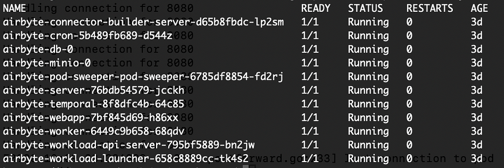
Wait a few minutes until the deployment is completed. Run the following command to check if the pods are running:
kubectl get pods --namespace dev-airbyte
Airbyte pods ready! Screen capture taken by me.
Accessing the Airbyte web app locally
After Airbyte is deployed you can get the container and port, and then run a port forwarding command to map a port in your local machine to the port in the Kubernetes web app pod. This will allow us to access the application using localhost.
export POD_NAME=$(kubectl get pods - namespace dev-airbyte -l "app.kubernetes.io/name=webapp" -o jsonpath="{.items[0].metadata.name}")
export CONTAINER_PORT=$(kubectl get pod - namespace dev-airbyte $POD_NAME -o jsonpath="{.spec.containers[0].ports[0].containerPort}")
kubectl - namespace dev-airbyte port-forward $POD_NAME 8080:$CONTAINER_PORT
echo "Visit http://127.0.0.1:8080 to use your application"
If you go to 127.0.0.1:8080 on your machine, you should see the application. Now, we can start adding data connectors!
Production Tip: Port forwarding works only for your local machine and must be done every time the shell is started. However, for data teams in real scenarios, Kubernetes allows you to expose your application throughout a virtual private network. For that, you will need to switch to Airbyte Self-managed enterprise which provides Single Sign-On with Cloud identity providers like Azure Active Directory to secure your workspace.
Setting up the data source
The provider for the data in this exercise is called Tiingo, which serves very valuable information from the companies in the stock market. They offer a free license that will give you access to the end-of-day prices endpoint for any asset and fundamental analysis for companies in the DOW 30. Be mindful that with the free license, their data are for your eyes only. If you want to share your creations based on Tiingo, you must pay for a commercial license. For now, I will use the free version and guide you through the tutorial without showing their actual stock data to remain compliant with their rules.
Create the account. Then, copy the API key provided to you. We are now ready to set up the source in Airbyte.
Creating a data source in Airbyte
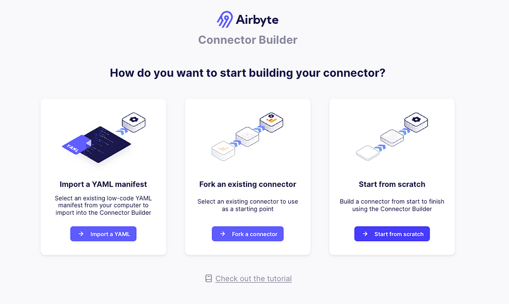
In the Airbyte app, go to Builder > Start from Scratch.
Airbyte connector builder screen. Image captured by me.
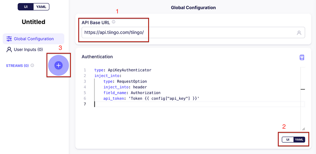
In the API Base URL write https://api.tiingo.com/tiingo/and for the configuration click on the YAML button. Enter the following:
This will allow the API token to be inserted in the header of every request. Now, let’s add your first stream by clicking on the plus icon (+) on the left. See the image below for guidance.
Building the data source. Global Configuration. Image captured by me.
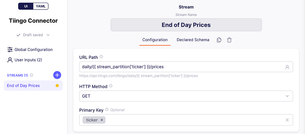
URL and stream partitioning
At the top write End of Day Prices. This will be our stream name and the URL path will be:
daily/{{ stream_partition['ticker'] }}/prices
What is this placeholder between {{}}? These are variables filled by Airbyte at runtime. In this case, Airbyte supports what they call stream partitioning, which allows the connector to make as many requests as the number of values you have on your partition array.
Defining URL path and primary key. Image captured by me.
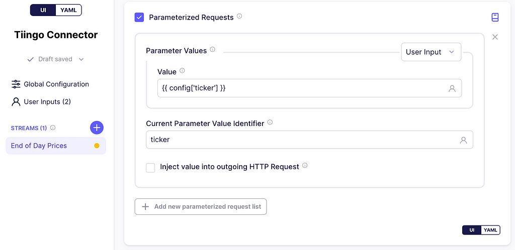
Scroll down to parameterized requests, and check the box. In the parameter values dropdown, click User Input, and on the value textbox enter:
{{ config['tickers_arr'] }}
Notice that the config variable used here is also referenced in the API Key in the global configuration. This variable holds the user inputs. Moreover, the user input tickers_arr will hold an array of stock IDs.
Next, on the Current Parameter Value Identifier textbox enter ticker. This is the key that is added to the stream_partition variable and references a single stock ID from the array tickers_arr for a single HTTP request. Below you can find screenshots of this process.
Defining the parameterized requests. Image captured by me.
We are going to test it with 4 stock tickers:
BA for Boeing Corp
CAT for Caterpillar
CVX for Chevron Corp
KO for Coca-Cola
With the stream partitioning set up, the connector will make 4 requests to the Tiingo server as follows:
Production Tip: Airbyte supports a parent stream, which allows us to get the list for the partitioning using a request to some other endpoint, instead of issuing the array elements ourselves. We are not doing that in this exercise, but you can check it out here.
Incremental Sync
Airbyte supports syncing data in Incremental Append mode i.e.: syncing only new or modified data. This prevents re-fetching data that you have already replicated from a source. If the sync is running for the first time, it is equivalent to a Full Refresh since all data will be considered as new.
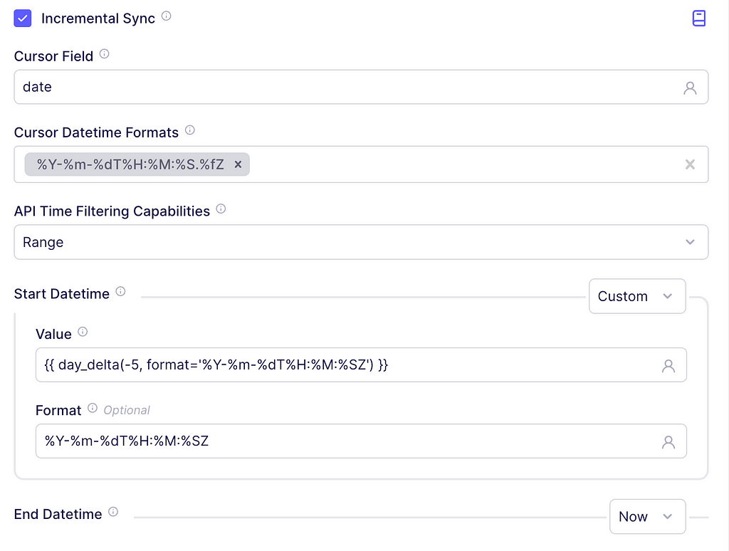
To implement this in our connector, scroll to Incremental Sync and check the box. In the cursor field textbox write date since, according to the documentation, that is the name of the date field indicating when the asset was updated. For the cursor DateTime Formats, enter
%Y-%m-%dT%H:%M:%S.%fZ
This is the output format suggested by the API docs.
In the Start DateTime dropdown click Custom and on the textbox enter the following:
{{ day_delta(-1, format='%Y-%m-%dT%H:%M:%SZ') }}
It will tell Airbyte to insert the date corresponding to yesterday. For the End Datetime leave the dropdown in Now to get data from the start date, up until today. The screenshot below depicts these steps.
Adding Incremental Start Datetime and End Datetime. Image captured by me.
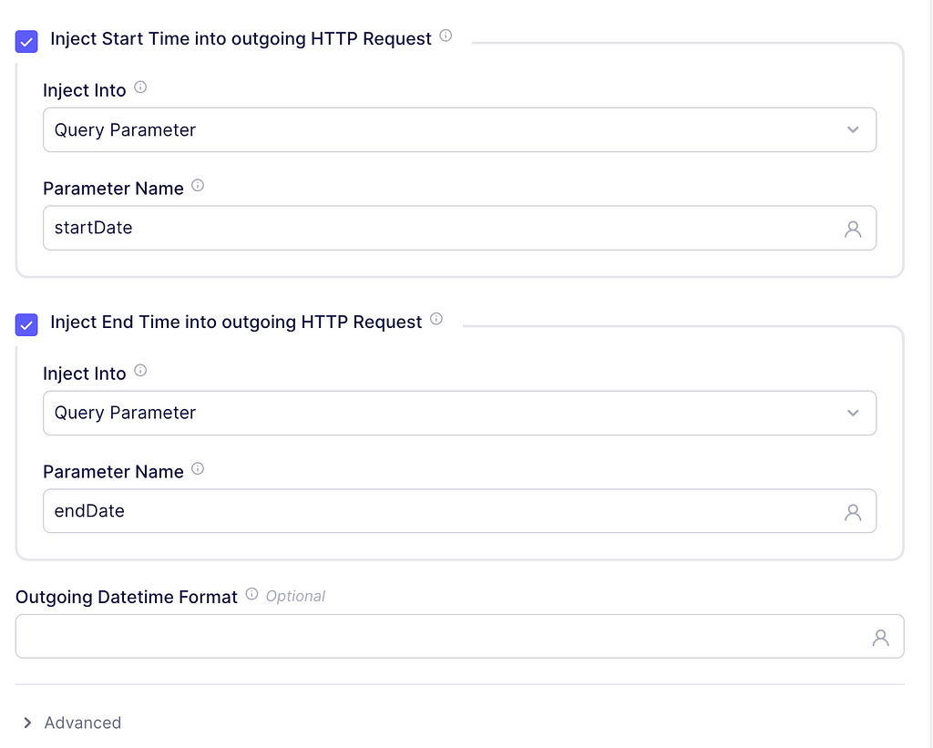
Finally, check the boxes to inject the start and end time into the outgoing HTTP request. The parameter names should be startDate and endDate, respectively. These parameter names come from Tiingo documentation as well. An example request will now look like:
Start and End Time parameters for our incremental loads. Image captured by me.
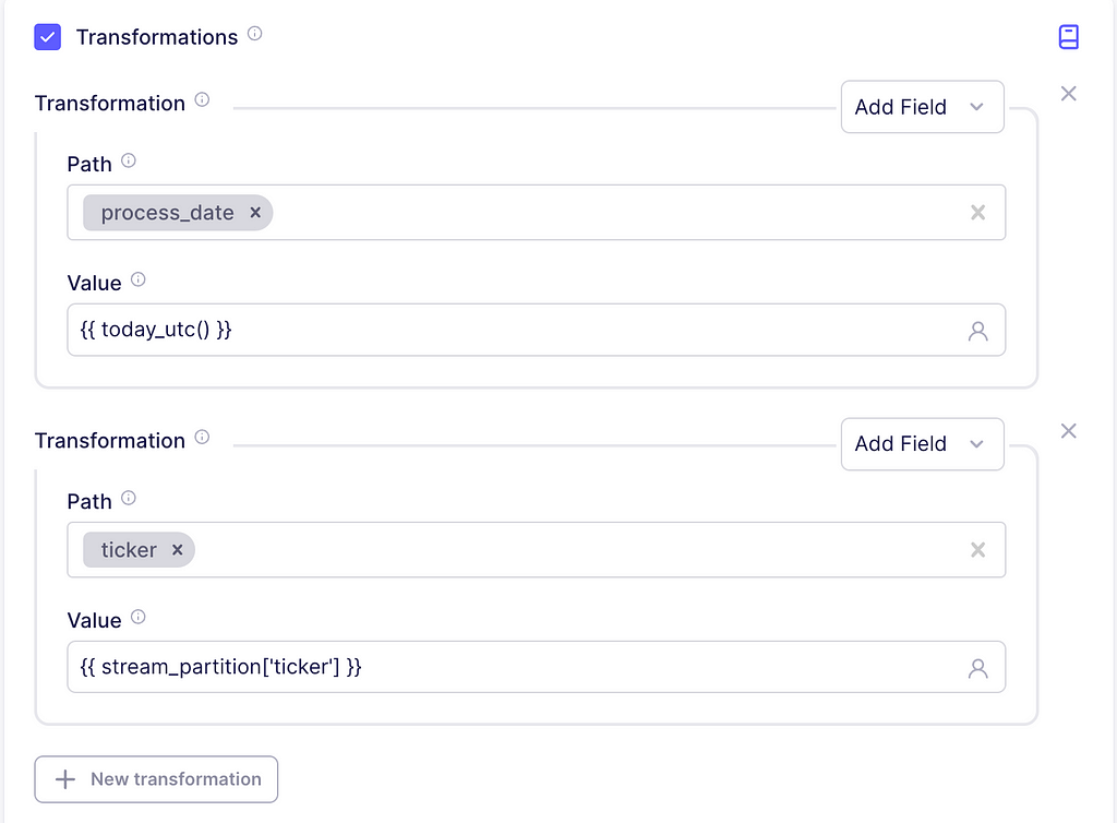
Control Fields
We are going to insert some information to enrich the data. For this, scroll to the transformations section and check the box. Inside the transformation dropdown, click on Add Field. The path is just the column name to be added, write process_date with the value {{ today_utc() }}. This will just indicate the timestamp for which the records were ingested into our system.
Now, according to the documentation, the ticker of the asset is not returned in the response, but we can easily add it using an additional transformation. So, for path, write ticker and the value should be {{ stream_partition[‘ticker’] }}. This will add the ticker value of the current stream partition as a column.
Adding our control fields to the API response. Image captured by me.
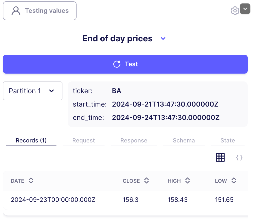
Testing
On the Testing values button, enter the list of tickers. A comma separates each ticker: BA, CAT, CVX, KO.
You should see something similar to the following image.
Notice the two example partitions. These are two separate, parameterized requests that Airbyte performed. You can also get information about the actual content in your request, the generated schema of the data, and state information.
Go to the top right corner and click publish to save this connector. Give it any name you want, I just called it Tiingo Connector.
Connecting Airbyte to the object store
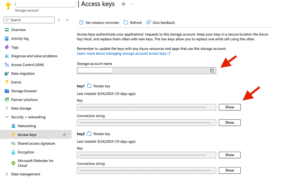
Let’s return to our storage service, go to Security + Networking > Access keys. Copy the account name and one of the access keys. Note: we need the access key, not the connection string.
Getting the access keys for the azure storage account. Image captured by me.
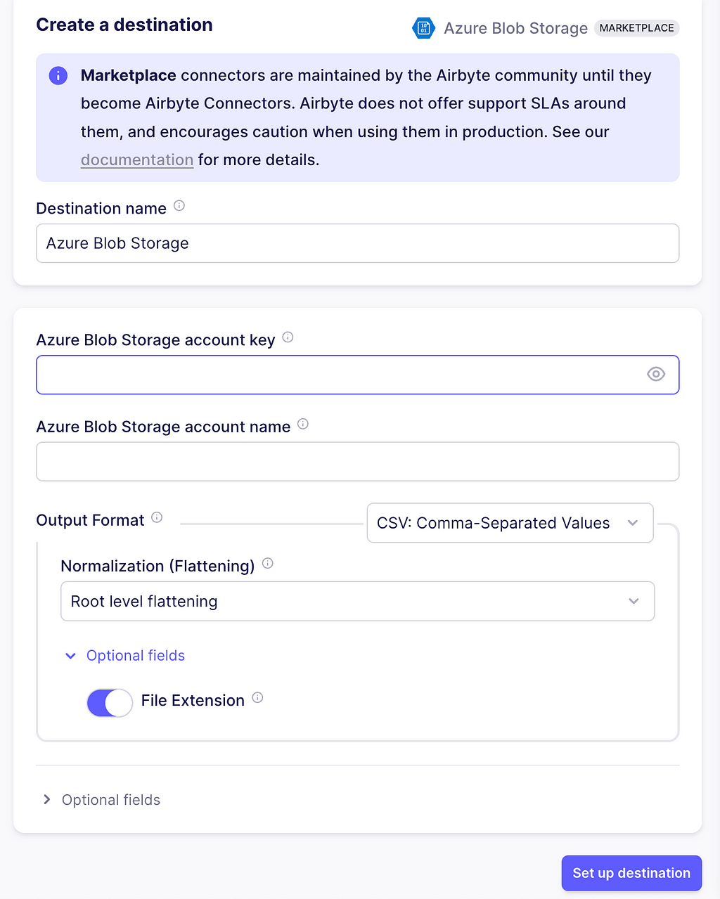
Next, go to your Airbyte app, select Destinations> Marketplace, and click Azure Blob Storage. Enter the account name, account key, and leave the other configurations as in the image. Additionally, in the Optional fields, enter the name of the container you created. Next, click on Set up destination.
Setting up the destination in Airbyte. Image captured by me.
Production Tip: Data assets from your organization need to be secured so that the individuals or teams have access to only the files they need. You can set up role-based access control at the storage account level with the Access Control (IAM) button, and also set Access Control Lists (ACLs) when right clicking folders, containers, or files.
Creating a connection from source to destination
There are four steps to build a connection in Airbyte and it will use the Tiingo Connector and the Azure Storage.
Defining the source
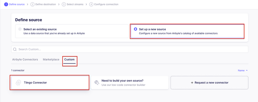
In the Airbyte app, go to connections and create one. The first step is to set up the source. Click Set up a new source. Then, on the Custom tab, select the Tiingo connector we just created.
Creating a source for the connection. Image captured by me.
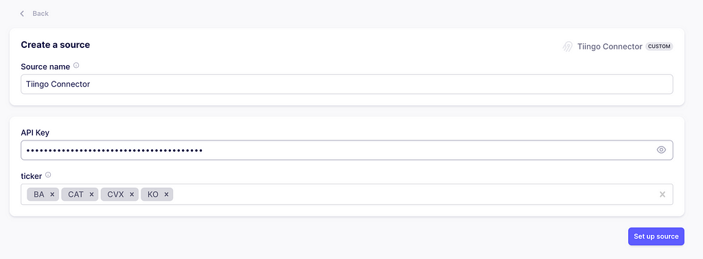
It will prompt you to enter the API Keys and stock tickers. Just copy the ones you used while testing the source. Now click on Set up source. It will test the connector with your configuration.
Adding user inputs for the source. Image captured by me.
Defining the destination
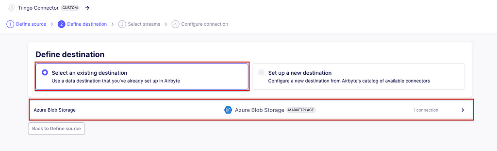
Once it has passed, we will set up the destination, which is the one created in the above section. At this time, Airbyte will also test the destination.
Adding the destination for the connection. Image captured by me.
Defining streams
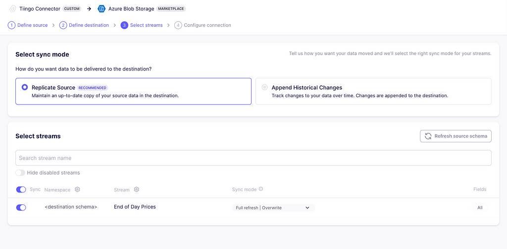
The third step is to select the streams and the sync mode. As we only defined one stream called End of Day Prices, this is the only one available. As for the sync modes, these are the options available for this exercise:
Full Refresh | Overwrite: This mode will retrieve all the data and replace any existing data in the destination.
Full Refresh | Append: This mode will also retrieve all of the data, but it will append the new data to the destination. You must deduplicate or transform your data properly to suit your needs afterward.
Incremental | Append: This mode requests data given the incremental conditions we defined while building the connector. Then, it will append the data to the destination.
You can read more about synch modes here. For now, choose Incremental | Append.
Selecting the streams to ingest. Image captured by me.
Final connection configurations
Here you can define the schedule you want, plus other additional settings. Click finish and sync to prompt your first data extraction and ingestion.
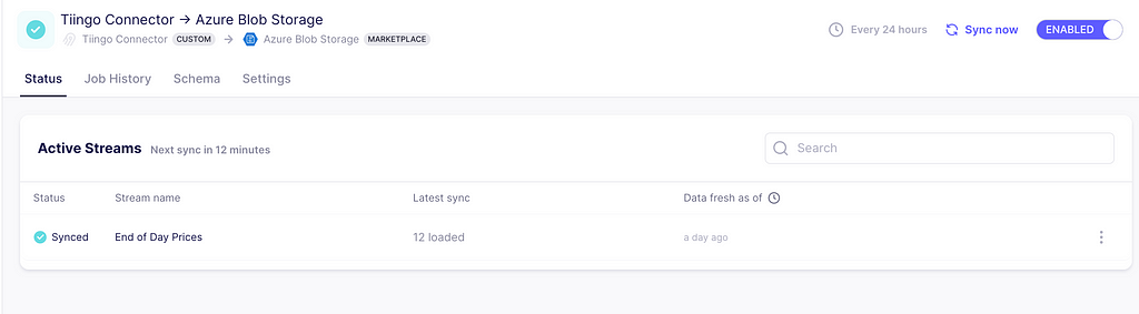
Running the first synching process. Image captured by me.
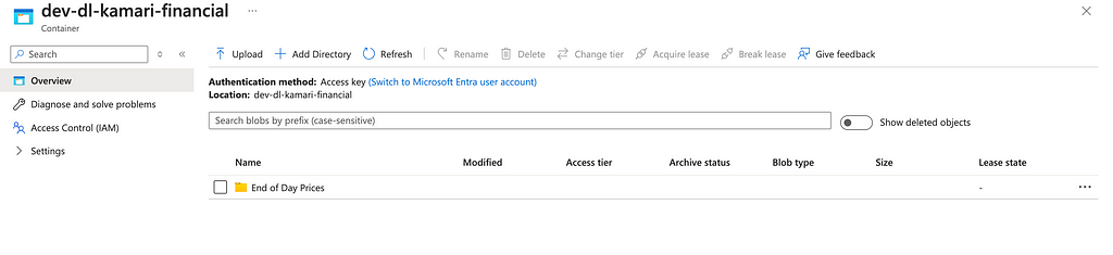
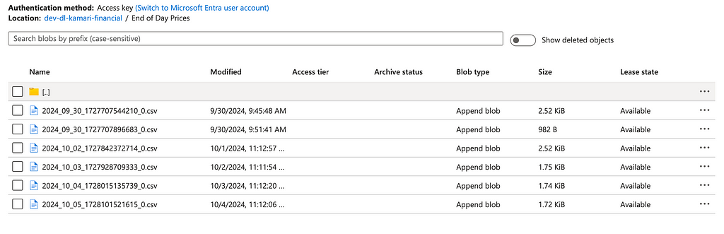
And that’s it! The data is now ingested. Head back to the storage container and you will see a new folder with one CSV file. With the append mode chosen, whenever a sync is triggered, a new file appears in the folder.
A new folder with the name of the stream is created. Image captured by me.Data files as a result of multiple syncs in Airbyte. Image captured by me.
Conclusion
You can clearly see the power of these kinds of tools. In this case, Airbyte allows you to get started with ingesting critical data in a matter of minutes with production-grade connectors, without the need to maintain large amounts of code. In addition, it allows incremental and full refresh modes with append or overwrite capabilities. In this exercise, only the Rest API sources were demonstrated, but there are many other source types, such as traditional databases, data warehouses, object stores, and many other platforms. Finally, it also offers a variety of destinations where your data can land and be analyzed further, greatly speeding up the development process and allowing you to take your products to market faster!
Thank you for reading this article! If you enjoyed it, please give it a clap and share. I do my best to write about the things I learn in the data world as an appreciation for this community that has taught me so much.
We use cookies on our website to give you the most relevant experience by remembering your preferences and repeat visits. By clicking “Accept”, you consent to the use of ALL the cookies.
This website uses cookies to improve your experience while you navigate through the website. Out of these, the cookies that are categorized as necessary are stored on your browser as they are essential for the working of basic functionalities of the website. We also use third-party cookies that help us analyze and understand how you use this website. These cookies will be stored in your browser only with your consent. You also have the option to opt-out of these cookies. But opting out of some of these cookies may affect your browsing experience.
Necessary cookies are absolutely essential for the website to function properly. These cookies ensure basic functionalities and security features of the website, anonymously.
Cookie
Duration
Description
cookielawinfo-checkbox-analytics
11 months
This cookie is set by GDPR Cookie Consent plugin. The cookie is used to store the user consent for the cookies in the category "Analytics".
cookielawinfo-checkbox-functional
11 months
The cookie is set by GDPR cookie consent to record the user consent for the cookies in the category "Functional".
cookielawinfo-checkbox-necessary
11 months
This cookie is set by GDPR Cookie Consent plugin. The cookies is used to store the user consent for the cookies in the category "Necessary".
cookielawinfo-checkbox-others
11 months
This cookie is set by GDPR Cookie Consent plugin. The cookie is used to store the user consent for the cookies in the category "Other.
cookielawinfo-checkbox-performance
11 months
This cookie is set by GDPR Cookie Consent plugin. The cookie is used to store the user consent for the cookies in the category "Performance".
viewed_cookie_policy
11 months
The cookie is set by the GDPR Cookie Consent plugin and is used to store whether or not user has consented to the use of cookies. It does not store any personal data.
Functional cookies help to perform certain functionalities like sharing the content of the website on social media platforms, collect feedbacks, and other third-party features.
Performance cookies are used to understand and analyze the key performance indexes of the website which helps in delivering a better user experience for the visitors.
Analytical cookies are used to understand how visitors interact with the website. These cookies help provide information on metrics the number of visitors, bounce rate, traffic source, etc.
Advertisement cookies are used to provide visitors with relevant ads and marketing campaigns. These cookies track visitors across websites and collect information to provide customized ads.