Category: Artificial Intelligence

  • Linear Discriminant Analysis (LDA)

    Linear Discriminant Analysis (LDA)

    Ingo Nowitzky

    Discover how LDA helps identify critical data features

    Classification of LDA within AI and ML Methods | image by author

    This article aims to explore Linear Discriminant Analysis (LDA), focusing on its core ideas, its mathematical implementation in code, and a practical example from manufacturing.
    I hope you’re on board. Let’s get started!

    Who works with industrial data in practice will be familiar with this situation: The datasets usually have many features, and it is often unclear which of the features are important and which are less. “Important” is a relative term in this context. Often, the goal is to differentiate the datasets from each other, i.e., to classify them. A very typical task is to distinguish good parts from bad parts and to identify the causes (aka features) that lead to the failure of the parts.

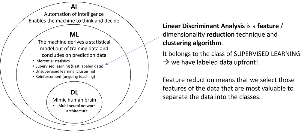
    A commonly used method is the well-known Principal Component Analysis (PCA). While PCA belongs to the unsupervised methods, the less widespread LDA is a supervised method and thus learns from labeled data. Therefore, it is particularly suited for explaining failure patterns from large datasets.

    1. Goal and Principle of LDA

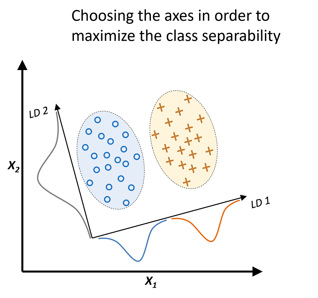
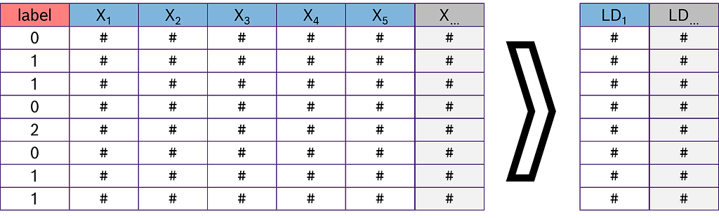
    The goal of LDA is to linearly combine the features of the data so that the labels of the datasets are best separated from each other, and the number of new features is reduced to a predefined count. In AI jargon, this is typically referred to as a projection to a lower-dimensional space.

    Principle of LDA | image modified from Raschka/Mirjalili, 2019

    Excursus: What is dimensionality and what is dimensionality reduction?

    Dimensions and graphical representation | image by author

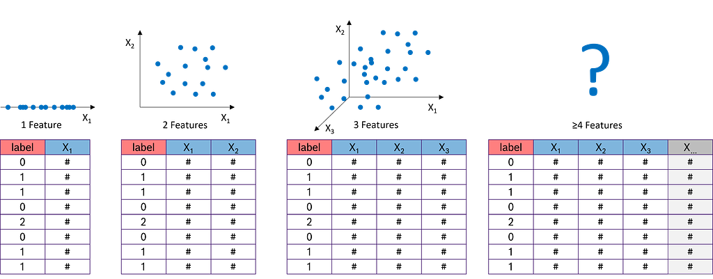
    Dimensionality refers to the number of features in a dataset.
    With just one measurement (or feature), such as the tool temperature from an injection molding machine, we can represent it on a number line. Two features, like temperature and tool pressure, are still manageable: we can easily plot the data on an x-y chart. With three features — temperature, tool pressure, and injection pressure — things get more interesting, but we can still plot the data in a 3D x-y-z chart. However, when we add more features, such as viscosity, electrical conductivity, and others, the complexity increases.

    Dimensionality reduction | image by author

    In practice, datasets often contain hundreds or even thousands of features. This presents a challenge because many machine learning algorithms perform poorly as datasets grow too large. Additionally, the amount of data required increases exponentially with the number of dimensions to achieve statistical significance. This phenomenon is known as the “curse of dimensionality.” These factors make it essential to determine which features are relevant and to eliminate the less meaningful ones early in the data science process.

    2. How does LDA work?

    The process of Linear Discriminant Analysis (LDA) can be broken down into five key steps.

    Step 1: Compute the d-dimensional mean vectors for each of the k classes separately from the dataset.

    Remember that LDA is a supervised machine learning technique, meaning we can utilize the known labels. In the first step, we calculate the mean vectors mean_c for all samples belonging to a specific class c. To do this, we filter the feature matrix by class label and compute the mean for each of the d features. As a result, we obtain k mean vectors (one for each of the k classes), each with a length of d (corresponding to the d features).

    Label vector Y and feature matrix X | image by author

    Step 2: Compute the scatter matrices (between-class scatter matrix and within-class scatter matrix).

    The within-class scatter matrix measures the variation among samples within the same class. To find a subspace with optimal separability, we aim to minimize the values in this matrix. In contrast, the between-class scatter matrix measures the variation between different classes. For optimal separability, we aim to maximize the values in this matrix.
    Intuitively, within-class scatter looks at how compact each class is, whereas between-class scatter examines how far apart different classes are.

    Within-class and between-class scatter matrices | image by author

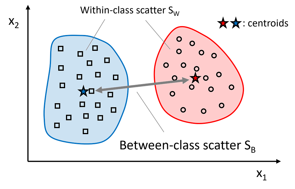
    Let’s start with the within-class scatter matrix S_W. It is calculated as the sum of the scatter matrices S_c for each individual class:

    The between-class scatter matrix S_B is derived from the differences between the class means mean_c and the overall mean of the entire dataset:

    where mean refers to the mean vector calculated over all samples, regardless of their class labels.

    Step 3: Calculate the eigenvectors and eigenvalues for the ratio of S_W​ and S_B​.

    As mentioned, for optimal class separability, we aim to maximize S_B​ and minimize S_W​. We can achieve both by maximizing the ratio S_B/S_W​. In linear algebra terms, this ratio corresponds to the scatter matrix S_W⁻¹ S_B​, which is maximized in the subspace spanned by the eigenvectors with the highest eigenvalues. The eigenvectors define the directions of this subspace, while the eigenvalues represent the magnitude of the distortion. We will select the m eigenvectors associated with the highest eigenvalues.

    Subspace spanned by eigenvectors | image by author

    Step 4: Sort the eigenvectors in descending order of their corresponding eigenvalues, and select the m eigenvectors with the largest eigenvalues to form a d × m-dimensional transformation matrix W.

    Remember, our goal is not only to project the data into a subspace that enhances class separability but also to reduce dimensionality. The eigenvectors will define the axes of our new feature subspace. To decide which eigenvectors to discard for the lower-dimensional subspace, we need to examine their corresponding eigenvalues. In simple terms, the eigenvectors with the smallest eigenvalues contribute the least to class separation, and these are the ones we want to drop. The typical approach is to rank the eigenvalues in descending order and select the top m eigenvectors. m is a freely chosen parameter. The larger m, the less information is lost during the transformation.

    After sorting the eigenpairs by decreasing eigenvalues and selecting the top m pairs, the next step is to construct the d × m-dimensional transformation matrix W. This is done by stacking the m selected eigenvectors horizontally, resulting in the matrix W:

    The first column of W represents the eigenvector corresponding to the highest eigenvalue, the second column represents the eigenvector corresponding to the second highest eigenvalue, and so on.

    Step 5: Use W to project the samples onto the new subspace.

    In the final step, we use the d × m-dimensional transformation matrix W, which we composed from the top m selected eigenvectors, to project our samples onto the new subspace:

    where X is the initial n × d-dimensional feature matrix representing our samples, and Z is the newly transformed n × m-dimensional feature matrix in the new subspace. This means that the selected eigenvectors serve as the “recipes” for transforming the original features into the new features (the Linear Discriminants): The eigenvector with the highest eigenvalue provides the transformation recipe for LD1, the eigenvector with the second highest eigenvalue corresponds to LD2, and so on.

    Projection of X onto the linear discriminants LD

    3. Implementing Linear Discriminant Analysis (LDA) from Scratch

    To demonstrate the theory and mathematics in action, we will program our own LDA from scratch using only numpy.

    import numpy as np


    class LDA_fs:
    """
    Performs a Linear Discriminant Analysis (LDA)

    Methods
    =======
    fit_transform():
    Fits the model to the data X and Y, derives the transformation matrix W
    and projects the feature matrix X onto the m LDA axes
    """

    def __init__(self, m):
    """
    Parameters
    ==========
    m : int
    Number of LDA axes onto which the data will be projected

    Returns
    =======
    None
    """
    self.m = m

    def fit_transform(self, X, Y):
    """
    Parameters
    ==========
    X : array(n_samples, n_features)
    Feature matrix of the dataset
    Y = array(n_samples)
    Label vector of the dataset

    Returns
    =======
    X_transform : New feature matrix projected onto the m LDA axes

    """

    # Get number of features (columns)
    self.n_features = X.shape[1]
    # Get unique class labels
    class_labels = np.unique(Y)
    # Get the overall mean vector (independent of the class labels)
    mean_overall = np.mean(X, axis=0) # Mean of each feature
    # Initialize both scatter matrices with zeros
    SW = np.zeros((self.n_features, self.n_features)) # Within scatter matrix
    SB = np.zeros((self.n_features, self.n_features)) # Between scatter matrix

    # Iterate over all classes and select the corresponding data
    for c in class_labels:
    # Filter X for class c
    X_c = X[Y == c]
    # Calculate the mean vector for class c
    mean_c = np.mean(X_c, axis=0)
    # Calculate within-class scatter for class c
    SW += (X_c - mean_c).T.dot((X_c - mean_c))
    # Number of samples in class c
    n_c = X_c.shape[0]
    # Difference between the overall mean and the mean of class c --> between-class scatter
    mean_diff = (mean_c - mean_overall).reshape(self.n_features, 1)
    SB += n_c * (mean_diff).dot(mean_diff.T)

    # Determine SW^-1 * SB
    A = np.linalg.inv(SW).dot(SB)
    # Get the eigenvalues and eigenvectors of (SW^-1 * SB)
    eigenvalues, eigenvectors = np.linalg.eig(A)
    # Keep only the real parts of eigenvalues and eigenvectors
    eigenvalues = np.real(eigenvalues)
    eigenvectors = np.real(eigenvectors.T)

    # Sort the eigenvalues descending (high to low)
    idxs = np.argsort(np.abs(eigenvalues))[::-1]
    self.eigenvalues = np.abs(eigenvalues[idxs])
    self.eigenvectors = eigenvectors[idxs]
    # Store the first m eigenvectors as transformation matrix W
    self.W = self.eigenvectors[0:self.m]

    # Transform the feature matrix X onto LD axes
    return np.dot(X, self.W.T)

    4. Applying LDA to an Industrial Dataset

    To see LDA in action, we will apply it to a typical task in the production environment. We have data from a simple manufacturing line with only 7 stations. Each of these stations sends a data point (yes, I know, only one data point is highly unrealistic). Unfortunately, our line produces a significant number of defective parts, and we want to find out which stations are responsible for this.

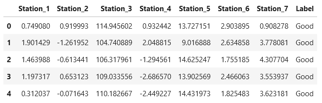
    First, we load the data and take an initial look.

    import pandas as pd

    # URL to Github repository
    url = "https://raw.githubusercontent.com/IngoNowitzky/LDA_Medium/main/production_line_data.csv"

    # Read csv to DataFrame
    data = pd.read_csv(url)

    # Print first 5 lines
    data.head()

    Next, we study the distribution of the data using the .describe() method from Pandas.

    # Show average, min and max of numerical values
    data.describe()

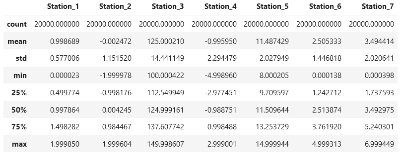
    We see that we have 20,000 data points, and the measurements range from -5 to +150. Hence, we note for later that we need to normalize the dataset: the different magnitudes of the numerical values would otherwise negatively affect the LDA.
    How many good parts and how many bad parts do we have?

    # Count the number of good and bad parts
    label_counts = data['Label'].value_counts()

    # Display the results
    print("Number of Good and Bad Parts:")
    print(label_counts)

    We have 19,031 good parts and 969 defective parts. The fact that the dataset is so imbalanced is an issue for further analysis. Therefore, we select all defective parts and an equal number of randomly chosen good parts for the further processing.

    # Select all bad parts
    bad_parts = data[data['Label'] == 'Bad']

    # Randomly select an equal number of good parts
    good_parts = data[data['Label'] == 'Good'].sample(n=len(bad_parts), random_state=42)

    # Combine both subsets to create a balanced dataset
    balanced_data = pd.concat([bad_parts, good_parts])

    # Shuffle the combined dataset
    balanced_data = balanced_data.sample(frac=1, random_state=42).reset_index(drop=True)

    # Display the number of good and bad parts in the balanced dataset
    print("Number of Good and Bad Parts in the balanced dataset:")
    print(balanced_data['Label'].value_counts())

    Now, let’s apply our LDA from scratch to the balanced dataset. We use the StandardScaler from sklearn to normalize the measurements for each feature to have a mean of 0 and a standard deviation of 1. We choose only one linear discriminant axis (m=1) onto which we project the data. This helps us clearly see which features are most relevant in distinguishing good from bad parts, and we visualize the projected data in a histogram.

    import matplotlib.pyplot as plt
    from sklearn.preprocessing import StandardScaler

    # Separate features and labels
    X = balanced_data.drop(columns=['Label'])
    y = balanced_data['Label']

    # Normalize the features
    scaler = StandardScaler()
    X_scaled = scaler.fit_transform(X)

    # Perform LDA
    lda = LDA_fs(m=1) # Instanciate LDA object with 1 axis
    X_lda = lda.fit_transform(X_scaled, y) # Fit the model and project the data

    # Plot the LDA projection
    plt.figure(figsize=(10, 6))
    plt.hist(X_lda[y == 'Good'], bins=20, alpha=0.7, label='Good', color='green')
    plt.hist(X_lda[y == 'Bad'], bins=20, alpha=0.7, label='Bad', color='red')
    plt.title("LDA Projection of Good and Bad Parts")
    plt.xlabel("LDA Component")
    plt.ylabel("Frequency")
    plt.legend()
    plt.show()

    # Examine feature contributions to the LDA component
    feature_importance = pd.DataFrame({'Feature': X.columns, 'LDA Coefficient': lda.W[0]})
    feature_importance = feature_importance.sort_values(by='LDA Coefficient', ascending=False)

    # Display feature importance
    print("Feature Contributions to LDA Component:")
    print(feature_importance)
    Feature matrix projected to one LD (m=1)
    Feature importance = How much do the stations contribute to class separation?

    The histogram shows that we can separate the good parts from the defective parts very well, with only a small overlap. This is already a positive result and indicates that our LDA was successful.

    The “LDA Coefficients” from the table “Feature Contributions to LDA Components” represent the eigenvector from the first (and only, since m=1) column of our transformation matrix W. They indicate the direction and magnitude with which the normalized measurements from the stations are projected onto the linear discriminant axis. The values in the table are sorted in descending order. We need to read the table from both the top and the bottom simultaneously because the absolute value of the coefficient indicates the significance of each station in separating the classes and, consequently, its contribution to the production of defective parts. The sign indicates whether a lower or higher measurement increases the likelihood of defective parts. Let’s take a closer look at our example:

    The largest absolute value is from Station 4, with a coefficient of -0.672. This means that Station 4 has the strongest influence on part failure. Due to the negative sign, higher positive measurements are projected towards a negative linear discriminant (LD). The histogram shows that a negative LD is associated with good (green) parts. Conversely, low and negative measurements at this station increase the likelihood of part failure.
    The second highest absolute value is from Station 2, with a coefficient of 0.557. Therefore, this station is the second most significant contributor to part failures. The positive sign indicates that high positive measurements are projected towards the positive LD. From the histogram, we know that a high positive LD value is associated with a high likelihood of failure. In other words, high measurements at Station 2 lead to part failures.
    The third highest coefficient comes from Station 7, with a value of -0.486. This makes Station 7 the third largest contributor to part failures. The negative sign again indicates that high positive values at this station lead to a negative LD (which corresponds to good parts). Conversely, low and negative values at this station lead to part failures.
    All other LDA coefficients are an order of magnitude smaller than the three mentioned, the associated stations therefore have no influence on part failure.

    Are the results of our LDA analysis correct? As you may have already guessed, the production dataset is synthetically generated. I labeled all parts as defective where the measurement at Station 2 was greater than 0.5, the value at Station 4 was less than -2.5, and the value at Station 7 was less than 3. It turns out that the LDA hit the mark perfectly!

    # Determine if a sample is a good or bad part based on the conditions
    data['Label'] = np.where(
    (data['Station_2'] > 0.5) & (data['Station_4'] < -2.5) & (data['Station_7'] < 3),
    'Bad',
    'Good'
    )

    5. Conclusion

    Linear Discriminant Analysis (LDA) not only reduces the complexity of datasets but also highlights the key features that drive class separation, making it highly effective for identifying failure causes in production systems. It is a straightforward yet powerful method with practical applications and is readily available in libraries like scikit-learn.

    To achieve optimal results, it is crucial to balance the dataset (ensure a similar number of samples in each class) and normalize it (mean of 0 and standard deviation of 1).
    The next time you work with a large dataset containing class labels and numerous features, why not give LDA a try?


    Linear Discriminant Analysis (LDA) was originally published in Towards Data Science on Medium, where people are continuing the conversation by highlighting and responding to this story.

    Originally appeared here:
    Linear Discriminant Analysis (LDA)

    Go Here to Read this Fast! Linear Discriminant Analysis (LDA)

  • Create a multimodal chatbot tailored to your unique dataset with Amazon Bedrock FMs

    Create a multimodal chatbot tailored to your unique dataset with Amazon Bedrock FMs

    Emmett Goodman

    In this post, we show how to create a multimodal chat assistant on Amazon Web Services (AWS) using Amazon Bedrock models, where users can submit images and questions, and text responses will be sourced from a closed set of proprietary documents.

    Originally appeared here:
    Create a multimodal chatbot tailored to your unique dataset with Amazon Bedrock FMs

    Go Here to Read this Fast! Create a multimodal chatbot tailored to your unique dataset with Amazon Bedrock FMs

  • Design secure generative AI application workflows with Amazon Verified Permissions and Amazon Bedrock Agents

    Design secure generative AI application workflows with Amazon Verified Permissions and Amazon Bedrock Agents

    Ram Vittal

    In this post, we demonstrate how to design fine-grained access controls using Verified Permissions for a generative AI application that uses Amazon Bedrock Agents to answer questions about insurance claims that exist in a claims review system using textual prompts as inputs and outputs.

    Originally appeared here:
    Design secure generative AI application workflows with Amazon Verified Permissions and Amazon Bedrock Agents

    Go Here to Read this Fast! Design secure generative AI application workflows with Amazon Verified Permissions and Amazon Bedrock Agents

  • How to Set Bid Guardrails in PPC Marketing

    How to Set Bid Guardrails in PPC Marketing

    Jose Parreño

    Without controls, bidding algorithms can be quite volatile. Learn how to protect performance through adding guardrails.

    Originally appeared here:
    How to Set Bid Guardrails in PPC Marketing

    Go Here to Read this Fast! How to Set Bid Guardrails in PPC Marketing

  • lintsampler: a new way to quickly get random samples from any distribution

    lintsampler: a new way to quickly get random samples from any distribution

    Aneesh Naik

    lintsampler is a pure Python package that can easily and efficiently generate random samples from any probability distribution.

    Full disclosure: I am one of the authors of lintsampler.

    Why you need lintsampler

    We often find ourselves in situations where we have a probability distribution (PDF) and we need to draw random samples it. For example, we might want to estimate some summary statistics or to create a population of particles for a simulation.

    If the probability distribution is a standard one, such as a uniform distribution or a Gaussian (normal) distribution, then the numpy/scipy ecosystem provides us with some easy ways to draw these samples, via the numpy.random or scipy.stats modules.

    However, out in the wild, we often encounter probability distributions that are not Gaussian. Sometimes, they are very not Gaussian. For example:

    A very non-Gaussian PDF. Contour lines are lines of equal density, separated by equal intervals in log-space. Image by author.

    How would we draw samples from this distribution?

    There are a few widely-used techniques to draw samples from arbitrary distributions like this, such as rejection sampling or Markov chain Monte Carlo (MCMC). These are excellent and reliable methods, with some handy Python implementations. For example, emcee is an MCMC sampler widely used in scientific applications.

    The problem with these existing techniques is that they require a fair amount of setup and tuning. With rejection sampling, one has to choose a proposal distribution, and a poor choice can make the procedure very inefficient. With MCMC one has to worry about whether the samples are converged, which typically requires some post-hoc testing to gauge.

    Enter lintsampler. It’s as easy as:

    from lintsampler import LintSampler
    import numpy as np

    x = np.linspace(xmin, xmax, ngrid)
    y = np.linspace(ymin, ymax, ngrid)
    sampler = LintSampler((x, y), pdf)
    pts = sampler.sample(N=100000)

    In this code snippet, we constructed 1D arrays along each of the two dimensions, then we fed them to the LintSampler object (imported from the lintsampler package) along with a pdf function representing the probability distribution we want to draw samples from. We didn’t spell out the pdf function in this snippet, but there are some fully self-contained examples in the docs.

    Now, pts is an array containing 100000 samples from the PDF. Here they are in a scatter plot:

    Scatter plot of points sampled from the weird PDF above (the latter is represented by the contour lines). Image by author.

    The point of this example was to demonstrate how easy it is to set up and use lintsampler. In certain cases, it is also much faster and more efficient than MCMC and/or rejection sampling. If you’re interested to find out how lintsampler works under the hood, read on. Otherwise, visit the docs, where there are instructions describing how to install and use lintsampler, including example notebooks with 1D, 2D, and 3D use cases, as well as descriptions of some of lintsampler’s additional features: quasi Monte Carlo sampling (a.k.a. low discrepancy sequencing), and sampling on an adaptive tree structure. There is also a paper published in the Journal of Open Source Software (JOSS) describing lintsampler.

    How lintsampler works

    Underlying lintsampler is an algorithm we call linear interpolant sampling. The theory section of the docs gives a more detailed and more mathematical description of how the algorithm works, but here it is in short.

    The example below illustrates what happens under the hood in lintsampler when you feed a PDF and a grid to the LintSampler class. We’ll take an easy example of a 2D Gaussian, but this methodology applies in any number of dimensions, and with much less friendly PDFs.

    • First, the PDF gets evaluated on the grid. In the example below, the grid has uneven spacings, just for fun.
    Left: 2D Gaussian PDF. Right: PDF evaluated on (uneven) grid. Image by author.
    • Having evaluated the PDF on the grid in this way, we can estimate the total probability of each grid cell according to the trapezium rule (i.e., volume of the cell multiplied by the average of its corner densities).
    • Within each grid cell, we can approximate the PDF with the bilinear interpolant between the cell corners:
    Gridded PDF filled in with (bi)linear interpolation. Image by author.
    • This linear approximation to the PDF can then be sampled very efficiently. Drawing a single sample is a two step process, illustrated in the figure below. First, choose a random cell from the probability-weighted list of cells (left-hand panel). Next, sample a point within the cell via inverse transform sampling (right-hand panel).
    Left: same as previous figure, with randomly chosen cell highlighted. Right: Zoom-in of highlighted cell, with sampled point illustrated. Image by author.

    It is worth understanding that the key step here is the linear approximation: we describe this, as well as more details of the inverse transform sampling process, in the lintsampler docs. Approximating the PDF to a linear function within grid each cell means it has a closed, analytic form for its quantile function (i.e., its inverse CDF), which means doing inverse transform sampling essentially boils down to drawing uniform samples and applying an algebraic function to them.

    The main thing the user needs to worry about is getting a decent grid resolution, so that the linear approximation is sufficient. What a good resolution is will vary from use case to use case, as demonstrated in some of the example notebooks in the lintsampler docs.

    Happy sampling!


    lintsampler: a new way to quickly get random samples from any distribution was originally published in Towards Data Science on Medium, where people are continuing the conversation by highlighting and responding to this story.

    Originally appeared here:
    lintsampler: a new way to quickly get random samples from any distribution

    Go Here to Read this Fast! lintsampler: a new way to quickly get random samples from any distribution

  • Bringing Structure to Your Data

    Dorian Drost

    Testing assumptions with path models

    In complicated path models, it might become difficult to find your way. Photo by Deva Darshan on Unsplash

    Data Scientists often collect a multitude of variables and search for relationships between them. During this journey, it is helpful to have assumptions and hypotheses on how exactly variables relate to each other. Does a student’s motivation to study for the next exam influence their grades? Or do good grades lead to motivation to study at all? And what exactly are the behavioral patterns that motivated people show that lead to good grades in the end?

    To give some structure to questions like the aforementioned and to provide a tool to test them empirically, I want to explain path models, also called Structural Equation Models (SEMs) in this article. While in social sciences like psychology path models are commonly used, I feel they are not that prominent in other areas like data science and computer science. Hence I want to give an overview of the main concept of path analysis and introduce semopy, which is a package for applying path analysis in python. Throughout this article, we will analyze artificial data to showcase typical problems that can be solved with path models and introduce the concepts of moderators and mediators. Be aware that this data has been generated for demonstration purposes and may not be realistic in every detail.

    Research question

    Before analysing data, we need to have an idea what we search for. Photo by Ansia Lasa on Unsplash

    If we want to analyze data, we need to have a research question in mind that we want to investigate. For this article, let us investigate school children and the grades they achieve. We might be interested in factors that foster learning and achieving good grades. That could be the amount of fun they have in school, their feeling of belonging to class, their interest in the subject, their number of friends in the class, their relationship with the teacher, their intelligence and much more. So we go into different schools and collect data by handing out questionnaires on the feeling of belonging, the relationship with the teacher, the interest in the topic and the fun the pupils have in school, we conduct an IQ test with the pupils and we ask them how many friends they have. And of course we collect their grades in the exams.

    It all starts with data

    We now have data for all the variables shown here:

    Our next step is to investigate, how exactly the variables influence the grade. We can make different assumptions about the influences and we can verify these assumptions with the data. Let us start with the most trivial case, where we assume that each variable has a direct influence on the grades that is independent of all the other variables. For example, we would assume that higher intelligence leads to a better grade, no matter the interest in the topic or the fun the pupil has in school. A likewise relationship with the grades we would hypothesize for the other variables as well. Visually displayed, this relationship would look like this:

    Model assuming all variables directly influence the variable grades. Image by author.

    Each arrow describes an influence between the variables. We could also formulate this relationship as a weighted sum, like this:

    grades = a*feeling_of_belonging + b*number_of_friends + c*relationship_with_teacher + d*fun_in_school + e*intelligence + f*interest_in_topic

    Here a,b,c,d,e and f are weights that tell us, how strong the influence of the different variables is on our outcome grades. Okay, that is our assumption. Now we want to test this assumption given the data. Let’s say we have a data frame called data, where we have one column for each of the aforementioned variables. Then we can use semopy in python like this:

    import semopy 

    path = """
    grades ~ intelligence + interest_in_topic
    + feeling_of_belonging + relationship_with_teacher
    + fun_in_school + number_of_friends
    """

    m = semopy.Model(path)
    m.fit(data)

    In the last lines, we create a semopy.Model object and fit it with the data. The most interesting part is the variable path before. Here we specify the assumption we just had, namely that the variable grades is a combination of all the other variables. On the left part of the tilde (~) we have the variable that we expect to be dependent on the variables right to the tilde. Note that we didn’t explicitly specify the weights a,b,c,d,e and f. These weights are actually what we want to know, so let us run the following line to get a result:

    m.inspect()
    Results of the assumption that all variables directly influence the variable grade. Image by author.

    The weights a,b,c,d,e and f are what we see in the column Estimate. What information can we extract from this table? First, we see that some weights are bigger and some are smaller. For example, the feeling_of_belonging has the biggest weight (0.40), indicating that it has the strongest influence. Interest_in_topic, for example, has a much lower influence (0.08) and other variables like intelligence and number_of_friends have a weight of (almost) zero.

    Also, take a look at the p-value column. If you are familiar with statistical tests, you may already know how to interpret this. If not, don’t worry. There is a vast pile of literature on how to understand the topic of significance (this is what this column indicates) and I encourage you to deepen your knowledge about it. However, for the moment, we can just say that this column gives us some idea of how likely it is, that an effect we found is just random noise. For example, the influence of number_of_friends on grades is very small (-0.01) and it is very likely (0.42), that it is just a coincidence. Hence we would say there is no effect, although the weight is not exactly zero. The other way round, if the p-value is (close to) zero, we can assume that we indeed found an effect that is not just coincidence.

    Okay, so according to our analysis, there are three variables that have an influence on the grade, that are interest_in_topic (0.08), feeling_of_belonging (0.40) and relationship_with_teacher (0.19). The other variables have no influence. Is this our final answer?

    It is not! Remember, that the calculations performed by semopy were influenced by the assumptions we gave it. We said that we assume all variables to directly influence the grades independent of each other. But what if the actual relationship looks different? There are many other ways variables could influence each other, so let us come up with some different assumptions and thereby explore the concepts of mediators and moderators.

    Mediators

    Mediators can be like billard balls, where the one pushes the other. Photo by Steve Mushero on Unsplash

    Instead of saying that both number_of_friends and feeling_of_belonging influence grades directly, let us think in a different direction. If you don’t have any friends in class, you would not feel a sense of belonging to the class, would you? This feeling of (not) belonging might then influence the grade. So the relationship would rather look like this:

    Model assuming that number_of_friends influences feeling_of_belongig which in turn influences grades. Image by author.

    Note that the direct effect of number_of_friends on grades has vanished but we have an influence of number_of_friends on feeling_of_belonging, which in turn influences grades. We can take this assumption and let semopy test it:

    path = """
    feeling_of_belonging ~ number_of_friends
    grades ~ feeling_of_belonging
    """
    m = semopy.Model(path)
    m.fit(data)

    Here we said that feeling_of_belonging depends on number_of_friends and that grades depends on feeling_of_belonging. You see the output in the following. There is still a weight of 0.40 between feeling_of_belonging and grades, but now we also have a weight of 0.29 between number_of_friends and feeling_of_belonging. Looks like our assumption is valid. The number of friends influences the feeling of belonging and this, in turn, influences the grade.

    Results of the assumption of number_of_friends influencing feeling_of_belonging. Image by author.

    The kind of influence we have modelled here is called a mediator because one variable mediates the influence of another. In other words, number_of_friends does not have a direct influence on grades, but an indirect one, mediated through the feeling_of_belonging.

    Mediations can help us understand the exact ways and processes by which some variables influence each other. Students who have clear goals and ideas of what they want to become are less likely to drop out of high school, but what exactly are the behavioral patterns that lead to performing well in school? Is it learning more? Is it seeking help if one doesn’t understand a topic? These could both be mediators that (partly) explain the influence of clear goals on academic achievement.

    Moderators

    A moderator can be like a valve, that only allows a certain throughput. Photo by Igal Ness on Unsplash

    We just saw that assuming a different relationship between the variables helped describe the data more effectively. Maybe we can do something similar to make sense of the fact that intelligence has no influence on the grade in our data. This is surprising, as we would expect more intelligent pupils to reach higher grades on average, wouldn’t we? However, if a pupil is just not interested in the topic they wouldn’t spend much effort, would they? Maybe there is not a direct influence of intelligence on the grades, but there is a joint force of intelligence and interest. If pupils are interested in the topics, the more intelligent ones will receive higher grades, but if they are not interested, it doesn’t matter, because they don’t spend any effort. We could visualize this relationship like this:

    Model assuming that interest_in_topic moderatues the influence of intelligence on grades. Image by author.

    That is, we assume there is an effect of intelligence on the grades, but this effect is influenced by interest_in_topic. If interest is high, pupils will make use of their cognitive abilities and achieve higher grades, but if interest is low, they will not.

    If we want to test this assumption in semopy, we have to create a new variable that is the product of intelligence and interest_in_topic. Do you see how multiplying the variables reflects the ideas we just had? If interest_in_topic is near zero, the whole product is close to zero, no matter the intelligence. If interest_in_topic is high though, the product will be mainly driven by the high or low intelligence. So, we calculate a new column of our dataframe, call it intelligence_x_interest and feed semopy with our assumed relationship between this variable and the grades:

    path = """
    grades ~ intellgence_x_interest
    """
    m = semopy.Model(path)
    m.fit(data)

    And we find an effect:

    Result of the assumption of the product of intelligence and interest influencing grades. Image by author.

    Previously, intelligence had no effect on grades and interest_in_topic had a very small one (0.08). But if we combine them, we find a very big effect of 0.81. Looks like this combination of both variables describes our data much better.

    This interaction of variables is called moderation. We would say that interest_in_topic moderates the influence of intelligence on grades because the strength of the connection between intelligence and grades depends on the interest. Moderations can be important to understand how relations between variables differ in different circumstances or between different groups of participants. For example, longer experience in a job influences the salary positively, but for men, this influence is even stronger than for women. In this case, gender is the moderator for the effect of work experience on salary.

    Summing up

    If we combine all the previous steps, our new model looks like this:

    Full model with all the previous assumptions. Image by author.
    Results of the full model. Image by author.

    Now we have a more sophisticated and more plausible structure for our data. Note that fun_in_school still has no influence on the grades (hence I gave it a dashed line in the visualization above). Either there is none in the data, or we just did not find the correct interplay with the other variables yet. We might even be missing some interesting variables. Just like intelligence only made sense to look at in combination with interest_in_topic, maybe there is another variable that is required to understand the influence fun_in_school has on the grades. This shows you, that for path analysis, it is important to make sense of your data and have an idea what you want to investigate. It all starts with assumptions which you derive from theory (or sometimes from gut feeling) and which you then test with the data to better understand it.

    This is what path models are about. Let us sum up what we just learned.

    • Path models allow us to test assumptions on how exactly variables influence each other.
    • Mediations appear, if a variable a does not have a direct influence on a variable c, but influences another variable b, which then influences c.
    • We speak of moderations if the influence of a variable a on a variable c becomes stronger or less strong depending on another variable b. This can be modelled by calculating the product of variables.
    • Semopy can be used to test path models with given data in python.

    I hope I have been able to convince you of the usefulness of path models. What I showed you is just the very beginning of it though. Many more sophisticated assumptions can be tested with path models or other models derived from them, that go way beyond the scope of this article.

    References

    You can find semopy here:

    If you want to learn more about path analysis, Wikipedia can be a good entry point:

    I use this book for statistical background (unfortunately, it is available in German only):

    • Eid, M., Gollwitzer, M., & Schmitt, M. (2015). Statistik und Forschungsmethoden.

    This is how the data for this article has been generated:

    import numpy as np
    import pandas as pd

    np.random.seed(42)

    N = 7500

    def norm(x):
    return (x - np.mean(x)) / np.std(x)


    number_of_friends = [int(x) for x in np.random.exponential(2, N)]

    # let's assume the questionairs here had a range from 0 to 5
    relationship_with_teacher = np.random.normal(3.5,1,N)
    relationship_with_teacher = np.clip(relationship_with_teacher, 0,5)
    fun_in_school = np.random.normal(2.5, 2, N)
    fun_in_school = np.clip(fun_in_school, 0,5)

    # let's assume the interest_in_topic questionaire goes from 0 to 10
    interest_in_topic = 10-np.random.exponential(1, N)
    interest_in_topic = np.clip(interest_in_topic, 0, 10)

    intelligence = np.random.normal(100, 15, N)
    # normalize variables
    interest_in_topic = norm(interest_in_topic)
    fun_in_school = norm(fun_in_school)
    intelligence = norm(intelligence)
    relationship_with_teacher = norm(relationship_with_teacher)
    number_of_friends = norm(number_of_friends)

    # create dependend variables
    feeling_of_belonging = np.multiply(0.3, number_of_friends) + np.random.normal(0, 1, N)
    grades = 0.8 * intelligence * interest_in_topic + 0.2 * relationship_with_teacher + 0.4*feeling_of_belonging + np.random.normal(0,0.5,N)

    data = pd.DataFrame({
    "grades":grades,
    "intelligence":intelligence,
    "number_of_friends":number_of_friends,
    "fun_in_school":fun_in_school,
    "feeling_of_belonging": feeling_of_belonging,
    "interest_in_topic":interest_in_topic,
    "intellgence_x_interest" : intelligence * interest_in_topic,
    "relationship_with_teacher":relationship_with_teacher
    })

    Like this article? Follow me to be notified of my future posts.


    Bringing Structure to Your Data was originally published in Towards Data Science on Medium, where people are continuing the conversation by highlighting and responding to this story.

    Originally appeared here:
    Bringing Structure to Your Data

    Go Here to Read this Fast! Bringing Structure to Your Data

  • Nine Rules for Running Rust on Embedded Systems

    Nine Rules for Running Rust on Embedded Systems

    Carl M. Kadie

    Practical Lessons from Porting range-set-blaze to no_std

    Rust Running on Embedded — Source: https://openai.com/dall-e-2/. All other figures from the author.

    Do you want your Rust code to run everywhere — from large servers to web pages, robots, and even watches? In this final article of a three-part series, we’ll see how to use Rust to run on embedded devices using no_std.

    Porting your Rust project to a no_std environment allows you to target microcontrollers and deeply embedded systems, creating highly efficient software for constrained environments. For example, I used the upcoming version of range-set-blaze to create an LED animation sequencer and compositor that runs on a Raspberry Pi Pico:

    Running Rust without the standard library presents unique challenges. Without operating system support, features like file I/O, networking, and sometimes even dynamic memory allocation are unavailable. In this article, we’ll look at practical strategies to overcome these limitations.

    Porting Rust to no_std requires careful steps and choices, and missing any step can lead to failure. We’ll simplify the process by following these nine rules, which we will examine in detail:

    1. Confirm that your project works with WASM WASI and WASM in the Browser.
    2. Use target thumbv7m-none-eabi and cargo tree to identify and fix dependencies incompatible with no_std.
    3. Mark main (non-test) code no_std and alloc. Replace std:: with core:: and alloc::.
    4. Use Cargo features to let your main code use std optionally for file-related (etc.) functions.
    5. Understand why test code always uses the standard library.
    6. Create a simple embedded test project. Run it with QEMU.
    7. In Cargo.toml, add keywords and categories for WASM and no_std.
    8. [Optional] Use preallocated data types to avoid alloc.
    9. Add thumbv7m-none-eabi and QEMU to your CI (continuous integration) tests.

    Aside: These articles are based on a three-hour workshop that I presented at RustConf24 in Montreal. Thanks to the participants of that workshop. A special thanks, also, to the volunteers from the Seattle Rust Meetup who helped test this material. These articles replace an article I wrote last year with updated information.

    As with the first and second articles in this series, before we look at the rules one by one, let’s define our terms.

    • Native: Your home OS (Linux, Windows, macOS)
    • Standard library (std): Provides Rust’s core functionality — Vec, String, file input/output, networking, time.
    • WASM: WebAssembly (WASM) is a binary instruction format that runs in most browsers (and beyond).
    • WASI: WebAssembly System Interface (WASI) allows outside-the-browser WASM to access file I/O, networking (not yet), and time handling.
    • no_std: Instructs a Rust program not to use the full standard library, making it suitable for small, embedded devices or highly resource-constrained environments.
    • alloc: Provides heap memory allocation capabilities (Vec, String, etc.) in no_std environments, essential for dynamically managing memory.

    Based on my experience with range-set-blaze, a data structure project, here are the decisions I recommend, described one at a time. To avoid wishy-washiness, I’ll express them as rules.

    Rule 1: Confirm that your project works with WASM WASI and WASM in the Browser.

    Before porting your Rust code to an embedded environment, ensure it runs successfully in WASM WASI and WASM in the Browser. These environments expose issues related to moving away from the standard library and impose constraints like those of embedded systems. By addressing these challenges early, you’ll be closer to running your project on embedded devices.

    Environments in which we wish to run our code as a Venn diagram of progressively tighter constraints.

    Run the following commands to confirm that your code works in both WASM WASI and WASM in the Browser:

    cargo test --target wasm32-wasip1
    cargo test --target wasm32-unknown-unknown

    If the tests fail or don’t run, revisit the steps from the earlier articles in this series: WASM WASI and WASM in the Browser.

    The WASM WASI article also provides crucial background on understanding Rust targets (Rule 2), conditional compilation (Rule 4), and Cargo features (Rule 6).

    Once you’ve fulfilled these prerequisites, the next step is to see how (and if) we can get our dependencies working on embedded systems.

    Rule 2: Use target thumbv7m-none-eabi and cargo tree to identify and fix dependencies incompatible with no_std.

    To check if your dependencies are compatible with an embedded environment, compile your project for an embedded target. I recommend using the thumbv7m-none-eabi target:

    • thumbv7m — Represents the ARM Cortex-M3 microcontroller, a popular family of embedded processors.
    • none — Indicates that there is no operating system (OS) available. In Rust, this typically means we can’t rely on the standard library (std), so we use no_std. Recall that the standard library provides core functionality like Vec, String, file input/output, networking, and time.
    • eabi — Embedded Application Binary Interface, a standard defining calling conventions, data types, and binary layout for embedded executables.

    Since most embedded processors share the no_std constraint, ensuring compatibility with this target helps ensure compatibility with other embedded targets.

    Install the target and check your project:

    rustup target add thumbv7m-none-eabi
    cargo check --target thumbv7m-none-eabi

    When I did this on range-set-blaze, I encountered errors complaining about dependencies, such as:

    This shows that my project depends on num-traits, which depends on either, ultimately depending on std.

    The error messages can be confusing. To better understand the situation, run this cargo tree command:

    cargo tree --edges no-dev --format "{p} {f}"

    It displays a recursive list of your project’s dependencies and their active Cargo features. For example:

    range-set-blaze v0.1.6 (C:deldirbranchesrustconf24.nostd) 
    ├── gen_ops v0.3.0
    ├── itertools v0.13.0 default,use_alloc,use_std
    │ └── either v1.12.0 use_std
    ├── num-integer v0.1.46 default,std
    │ └── num-traits v0.2.19 default,i128,std
    │ [build-dependencies]
    │ └── autocfg v1.3.0
    └── num-traits v0.2.19 default,i128,std (*)

    We see multiple occurrences of Cargo features named use_std and std, strongly suggesting that:

    • These Cargo features require the standard library.
    • We can turn these Cargo features off.

    Using the techniques explained in the first article, Rule 6, we disable the use_std and std Cargo features. Recall that Cargo features are additive and have defaults. To turn off the default features, we use default-features = false. We then enable the Cargo features we want to keep by specifying, for example, features = [“use_alloc”]. The Cargo.toml now reads:

    [dependencies]
    gen_ops = "0.3.0"
    itertools = { version = "0.13.0", features=["use_alloc"], default-features = false }
    num-integer = { version = "0.1.46", default-features = false }
    num-traits = { version = "0.2.19", features=["i128"], default-features = false }

    Turning off Cargo features will not always be enough to make your dependencies no_std-compatible.

    For example, the popular thiserror crate introduces std into your code and offers no Cargo feature to disable it. However, the community has created no_std alternatives. You can find these alternatives by searching, for example, https://crates.io/search?q=thiserror+no_std.

    In the case of range-set-blaze, a problem remained related to crate gen_ops — a wonderful crate for conveniently defining operators such as + and &. The crate used std but didn’t need to. I identified the required one-line change (using the methods we’ll cover in Rule 3) and submitted a pull request. The maintainer accepted it, and they released an updated version: 0.4.0.

    Sometimes, our project can’t disable std because we need capabilities like file access when running on a full operating system. On embedded systems, however, we’re willing—and indeed must—give up such capabilities. In Rule 4, we’ll see how to make std usage optional by introducing our own Cargo features.

    Using these methods fixed all the dependency errors in range-set-blaze. However, resolving those errors revealed 281 errors in the main code. Progress!

    Rule 3: Mark main (non-test) code no_std and alloc. Replace std:: with core:: and alloc::.

    At the top of your project’s lib.rs (or main.rs) add:

    #![no_std]
    extern crate alloc;

    This means we won’t use the standard library, but we will still allocate memory. For range-set-blaze, this change reduced the error count from 281 to 52.

    Many of the remaining errors are due to using items in std that are available in core or alloc. Since much of std is just a re-export of core and alloc, we can resolve many errors by switching std references to core or alloc. This allows us to keep the essential functionality without relying on the standard library.

    For example, we get an error for each of these lines:

    use std::cmp::max;
    use std::cmp::Ordering;
    use std::collections::BTreeMap;

    Changing std:: to either core:: or (if memory related) alloc:: fixes the errors:

    use core::cmp::max;
    use core::cmp::Ordering;
    use alloc::collections::BTreeMap;

    Some capabilities, such as file access, are std-only—that is, they are defined outside of core and alloc. Fortunately, for range-set-blaze, switching to core and alloc resolved all 52 errors in the main code. However, this fix revealed 89 errors in its test code. Again, progress!

    We’ll address errors in the test code in Rule 5, but first, let’s figure out what to do if we need capabilities like file access when running on a full operating system.

    Rule 4: Use Cargo features to let your main code use std optionally for file-related (etc.) functions.

    If we need two versions of our code — one for running on a full operating system and one for embedded systems — we can use Cargo features (see Rule 6 in the first article). For example, let’s define a feature called foo, which will be the default. We’ll include the function demo_read_ranges_from_file only when foo is enabled.

    In Cargo.toml (preliminary):

    [features]
    default = ["foo"]
    foo = []

    In lib.rs (preliminary):

    #![no_std]
    extern crate alloc;

    // ...

    #[cfg(feature = "foo")]
    pub fn demo_read_ranges_from_file<P, T>(path: P) -> std::io::Result<RangeSetBlaze<T>>
    where
    P: AsRef<std::path::Path>,
    T: FromStr + Integer,
    {
    todo!("This function is not yet implemented.");
    }

    This says to define function demo_read_ranges_from_file only when Cargo feature foo is enabled. We can now check various versions of our code:

    cargo check # enables "foo", the default Cargo features
    cargo check --features foo # also enables "foo"
    cargo check --no-default-features # enables nothing

    Now let’s give our Cargo feature a more meaningful name by renaming foo to std. Our Cargo.toml (intermediate) now looks like:

    [features]
    default = ["std"]
    std = []

    In our lib.rs, we add these lines near the top to bring in the std library when the std Cargo feature is enabled:

    #[cfg(feature = "std")]
    extern crate std;

    So, lib.rs (final) looks like this:

    #![no_std]
    extern crate alloc;

    #[cfg(feature = "std")]
    extern crate std;

    // ...

    #[cfg(feature = "std")]
    pub fn demo_read_ranges_from_file<P, T>(path: P) -> std::io::Result<RangeSetBlaze<T>>
    where
    P: AsRef<std::path::Path>,
    T: FromStr + Integer,
    {
    todo!("This function is not yet implemented.");
    }

    We’d like to make one more change to our Cargo.toml. We want our new Cargo feature to control dependencies and their features. Here is the resulting Cargo.toml (final):

    [features]
    default = ["std"]
    std = ["itertools/use_std", "num-traits/std", "num-integer/std"]

    [dependencies]
    itertools = { version = "0.13.0", features = ["use_alloc"], default-features = false }
    num-integer = { version = "0.1.46", default-features = false }
    num-traits = { version = "0.2.19", features = ["i128"], default-features = false }
    gen_ops = "0.4.0"

    Aside: If you’re confused by the Cargo.toml format for specifying dependencies and features, see my recent article: Nine Rust Cargo.toml Wats and Wat Nots: Master Cargo.toml formatting rules and avoid frustration in Towards Data Science.

    To check that your project compiles both with the standard library (std) and without, use the following commands:

    cargo check # std
    cargo check --no-default-features # no_std

    With cargo check working, you’d think that cargo test would be straight forward. Unfortunately, it’s not. We’ll look at that next.

    Rule 5: Understand why test code always uses the standard library.

    When we compile our project with –no-default-features, it operates in a no_std environment. However, Rust’s testing framework always includes the standard library, even in a no_std project. This is because cargo test requires std; for example, the #[test] attribute and the test harness itself are defined in the standard library.

    As a result, running:

    # DOES NOT TEST `no_std`
    cargo test --no-default-features

    does not actually test the no_std version of your code. Functions from std that are unavailable in a true no_std environment will still be accessible during testing. For instance, the following test will compile and run successfully with –no-default-features, even though it uses std::fs:

    #[test]
    fn test_read_file_metadata() {
    let metadata = std::fs::metadata("./").unwrap();
    assert!(metadata.is_dir());
    }

    Additionally, when testing in std mode, you may need to add explicit imports for features from the standard library. This is because, even though std is available during testing, your project is still compiled as #![no_std], meaning the standard prelude is not automatically in scope. For example, you’ll often need the following imports in your test code:

    #![cfg(test)]
    use std::prelude::v1::*;
    use std::{format, print, println, vec};

    These imports bring in the necessary utilities from the standard library so that they are available during testing.

    To genuinely test your code without the standard library, you’ll need to use alternative methods that do not rely on cargo test. We’ll explore how to run no_std tests in the next rule.

    Rule 6: Create a simple embedded test project. Run it with QEMU.

    You can’t run your regular tests in an embedded environment. However, you can — and should — run at least one embedded test. My philosophy is that even a single test is infinitely better than none. Since “if it compiles, it works” is generally true for no_std projects, one (or a few) well-chosen test can be quite effective.

    To run this test, we use QEMU (Quick Emulator, pronounced “cue-em-you”), which allows us to emulate thumbv7m-none-eabi code on our main operating system (Linux, Windows, or macOS).

    Install QEMU.

    See the QEMU download page for full information:

    Linux/WSL

    • Ubuntu: sudo apt-get install qemu-system
    • Arch: sudo pacman -S qemu-system-arm
    • Fedora: sudo dnf install qemu-system-arm

    Windows

    • Method 1: https://qemu.weilnetz.de/w64. Run the installer (tell Windows that it is OK). Add “C:Program Filesqemu” to your path.
    • Method 2: Install MSYS2 from https://www.msys2.org/. Open MSYS2 UCRT64 terminal. pacman -S mingw-w64-x86_64-qemu. Add C:msys64mingw64bin to your path.

    Mac

    • brew install qemu or sudo port install qemu

    Test installation with:

    qemu-system-arm --version

    Create an embedded subproject.

    Create a subproject for the embedded tests:

    cargo new tests/embedded

    This command generates a new subproject, including the configuration file at tests/embedded/Cargo.toml.

    Aside: This command also modifies your top-level Cargo.toml to add the subproject to your workspace. In Rust, a workspace is a collection of related packages defined in the [workspace] section of the top-level Cargo.toml. All packages in the workspace share a single Cargo.lock file, ensuring consistent dependency versions across the entire workspace.

    Edit tests/embedded/Cargo.toml to look like this, but replace “range-set-blaze” with the name of your top-level project:

    [package]
    name = "embedded"
    version = "0.1.0"
    edition = "2021"

    [dependencies]
    alloc-cortex-m = "0.4.4"
    cortex-m = "0.7.7"
    cortex-m-rt = "0.7.3"
    cortex-m-semihosting = "0.5.0"
    panic-halt = "0.2.0"
    # Change to refer to your top-level project
    range-set-blaze = { path = "../..", default-features = false }

    Update the test code.

    Replace the contents of tests/embedded/src/main.rs with:

    // Based on https://github.com/rust-embedded/cortex-m-quickstart/blob/master/examples/allocator.rs
    // and https://github.com/rust-lang/rust/issues/51540
    #![feature(alloc_error_handler)]
    #![no_main]
    #![no_std]
    extern crate alloc;
    use alloc::string::ToString;
    use alloc_cortex_m::CortexMHeap;
    use core::{alloc::Layout, iter::FromIterator};
    use cortex_m::asm;
    use cortex_m_rt::entry;
    use cortex_m_semihosting::{debug, hprintln};
    use panic_halt as _;
    #[global_allocator]
    static ALLOCATOR: CortexMHeap = CortexMHeap::empty();
    const HEAP_SIZE: usize = 1024; // in bytes
    #[alloc_error_handler]
    fn alloc_error(_layout: Layout) -> ! {
    asm::bkpt();
    loop {}
    }

    #[entry]
    fn main() -> ! {
    unsafe { ALLOCATOR.init(cortex_m_rt::heap_start() as usize, HEAP_SIZE) }

    // Test(s) goes here. Run only under emulation
    use range_set_blaze::RangeSetBlaze;
    let range_set_blaze = RangeSetBlaze::from_iter([100, 103, 101, 102, -3, -4]);
    hprintln!("{:?}", range_set_blaze.to_string());
    if range_set_blaze.to_string() != "-4..=-3, 100..=103" {
    debug::exit(debug::EXIT_FAILURE);
    }

    debug::exit(debug::EXIT_SUCCESS);
    loop {}
    }

    Most of this main.rs code is embedded system boilerplate. The actual test code is:

    use range_set_blaze::RangeSetBlaze;
    let range_set_blaze = RangeSetBlaze::from_iter([100, 103, 101, 102, -3, -4]);
    hprintln!("{:?}", range_set_blaze.to_string());
    if range_set_blaze.to_string() != "-4..=-3, 100..=103" {
    debug::exit(debug::EXIT_FAILURE);
    }

    If the test fails, it returns EXIT_FAILURE; otherwise, it returns EXIT_SUCCESS. We use the hprintln! macro to print messages to the console during emulation. Since this is an embedded system, the code ends in an infinite loop to run continuously.

    Add supporting files.

    Before you can run the test, you must add two files to the subproject: build.rs and memory.x from the Cortex-M quickstart repository:

    Linux/WSL/macOS

    cd tests/embedded
    wget https://raw.githubusercontent.com/rust-embedded/cortex-m-quickstart/master/build.rs
    wget https://raw.githubusercontent.com/rust-embedded/cortex-m-quickstart/master/memory.

    Windows (Powershell)

    cd tests/embedded
    Invoke-WebRequest -Uri 'https://raw.githubusercontent.com/rust-embedded/cortex-m-quickstart/master/build.rs' -OutFile 'build.rs'
    Invoke-WebRequest -Uri 'https://raw.githubusercontent.com/rust-embedded/cortex-m-quickstart/master/memory.x' -OutFile 'memory.x'

    Also, create a tests/embedded/.cargo/config.toml with the following content:

    [target.thumbv7m-none-eabi]
    runner = "qemu-system-arm -cpu cortex-m3 -machine lm3s6965evb -nographic -semihosting-config enable=on,target=native -kernel"

    [build]
    target = "thumbv7m-none-eabi"

    This configuration instructs Cargo to use QEMU to run the embedded code and sets thumbv7m-none-eabi as the default target for the subproject.

    Run the test.

    Run the test with cargo run (not cargo test):

    # Setup
    # Make this subproject 'nightly' to support #![feature(alloc_error_handler)]
    rustup override set nightly
    rustup target add thumbv7m-none-eabi

    # If needed, cd tests/embedded
    cargo run

    You should see log messages, and the process should exit without error. In my case, I see: “-4..=-3, 100..=103”.

    These steps may seem like a significant amount of work just to run one (or a few) tests. However, it’s primarily a one-time effort involving mostly copy and paste. Additionally, it enables running tests in a CI environment (see Rule 9). The alternative — claiming that the code works in a no_std environment without ever actually running it in no_std—risks overlooking critical issues.

    The next rule is much simpler.

    Rule 7: In Cargo.toml, add keywords and categories for WASM and no_std.

    Once your package compiles and passes the additional embedded test, you may want to publish it to crates.io, Rust’s package registry. To let others know that it is compatible with WASM and no_std, add the following keywords and categories to your Cargo.toml file:

    [package]
    # ...
    categories = ["no-std", "wasm", "embedded"] # + others specific to your package
    keywords = ["no_std", "wasm"] # + others specific to your package

    Note that for categories, we use a hyphen in no-std. For keywords, no_std (with an underscore) is more popular than no-std. Your package can have a maximum of five keywords and five categories.

    Here is a list of categories and keywords of possible interest, along with the number of crates using each term:

    Good categories and keywords will help people find your package, but the system is informal. There’s no mechanism to check whether your categories and keywords are accurate, nor are you required to provide them.

    Next, we’ll explore one of the most restricted environments you’re likely to encounter.

    Rule 8: [Optional] Use preallocated data types to avoid alloc.

    My project, range-set-blaze, implements a dynamic data structure that requires memory allocation from the heap (via alloc). But what if your project doesn’t need dynamic memory allocation? In that case, it can run in even more restricted embedded environments—specifically those where all memory is preallocated when the program is loaded.

    The reasons to avoid alloc if you can:

    • Completely deterministic memory usage
    • Reduced risk of runtime failures (often caused by memory fragmentation)
    • Lower power consumption

    There are crates available that can sometimes help you replace dynamic data structures like Vec, String, and HashMap. These alternatives generally require you to specify a maximum size. The table below shows some popular crates for this purpose:

    I recommend the heapless crate because it provides a collection of data structures that work well together.

    Here is an example of code — using heapless — related to an LED display. This code creates a mapping from a byte to a list of integers. We limit the number of items in the map and the length of the integer list to DIGIT_COUNT (in this case, 4).

    use heapless::{LinearMap, Vec};
    // …
    let mut map: LinearMap<u8, Vec<usize, DIGIT_COUNT>, DIGIT_COUNT> = LinearMap::new();
    // …
    let mut vec = Vec::default();
    vec.push(index).unwrap();
    map.insert(*byte, vec).unwrap(); // actually copies

    Full details about creating a no_alloc project are beyond my experience. However, the first step is to remove this line (added in Rule 3) from your lib.rs or main.rs:

    extern crate alloc; // remove this

    Rule 9: Add thumbv7m-none-eabi and QEMU to your CI (continuous integration) tests.

    Your project is now compiling to no_std and passing at least one embedded-specific test. Are you done? Not quite. As I said in the previous two articles:

    If it’s not in CI, it doesn’t exist.

    Recall that continuous integration (CI) is a system that can automatically run tests every time you update your code. I use GitHub Actions as my CI platform. Here’s the configuration I added to .github/workflows/ci.yml to test my project on embedded platforms:

    test_thumbv7m_none_eabi:
    name: Setup and Check Embedded
    runs-on: ubuntu-latest
    steps:
    - name: Checkout
    uses: actions/checkout@v4
    - name: Set up Rust
    uses: dtolnay/rust-toolchain@master
    with:
    toolchain: stable
    target: thumbv7m-none-eabi
    - name: Install check stable and nightly
    run: |
    cargo check --target thumbv7m-none-eabi --no-default-features
    rustup override set nightly
    rustup target add thumbv7m-none-eabi
    cargo check --target thumbv7m-none-eabi --no-default-features
    sudo apt-get update && sudo apt-get install qemu qemu-system-arm
    - name: Test Embedded (in nightly)
    timeout-minutes: 1
    run: |
    cd tests/embedded
    cargo run

    By testing embedded and no_std with CI, I can be sure that my code will continue to support embedded platforms in the future.

    So, there you have it — nine rules for porting your Rust code to embedded. To see a snapshot of the whole range-set-blaze project after applying all nine rules, see this branch on Github.

    Here is what surprised me about porting to embedded:

    The Bad:

    • We cannot run our existing tests on embedded systems. Instead, we must create a new subproject and write (a few) new tests.
    • Many popular libraries rely on std, so finding or adapting dependencies that work with no_std can be challenging.

    The Good:

    • The Rust saying that “if it compiles, it works” holds true for embedded development. This gives us confidence in our code’s correctness without requiring extensive new tests.
    • Although no_std removes our immediate access to the standard library, many items continue to be available via core and alloc.
    • Thanks to emulation, you can develop for embedded systems without hardware.

    Thank you for joining me on this journey from WASI to WebAssembly in the browser and, finally, to embedded development. Rust has continued to impress me with its ability to run efficiently and safely across environments. As you explore these different domains, I hope you find Rust’s flexibility and power as compelling as I do. Whether you’re working on cloud servers, browsers, or microcontrollers, the tools we’ve discussed will help you tackle the challenges ahead with confidence.

    Interested in future articles? Please follow me on Medium. I write about Rust and Python, scientific programming, machine learning, and statistics. I tend to write about one article per month.


    Nine Rules for Running Rust on Embedded Systems was originally published in Towards Data Science on Medium, where people are continuing the conversation by highlighting and responding to this story.

    Originally appeared here:
    Nine Rules for Running Rust on Embedded Systems

    Go Here to Read this Fast! Nine Rules for Running Rust on Embedded Systems