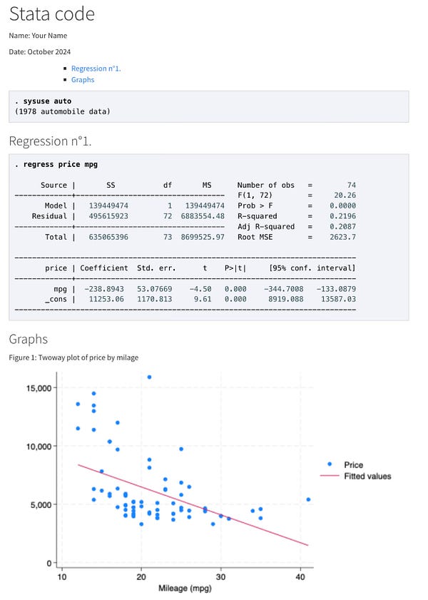
Create a shareable HTML document with your code, outputs, and graphs
Originally appeared here:
How to Export a Stata “Notebook” to HTML
Go Here to Read this Fast! How to Export a Stata “Notebook” to HTML

Create a shareable HTML document with your code, outputs, and graphs
Originally appeared here:
How to Export a Stata “Notebook” to HTML
Go Here to Read this Fast! How to Export a Stata “Notebook” to HTML


What is a Methodologist?
Traditionally, methodologists are those who study research methods, both qualitative and quantitative. Modern day methodologists (methodologist-analysts, methodologist-scientists, and methodologist-engineers) are the wielders of multiple approaches to complex problems. They are also conversant in the tools and technologies available for implementation, though often work best alongside true specialists in these areas (such as cloud architects, software developers, or data engineers).
I’ve written previously about the creative and systematic work involved in analytic methodology as a discipline. With the right personality and the proper technical or analytical exposure, the methodologist can be the most impactful technical role in an organization.
So, when your organization is hurting for data engineers, data scientists, and software engineers, why would you hire a methodologist? Better yet, who would even self-identify as a methodologist? (I would argue this guy is.)
A methodologist is someone who…
We’ve heard that innovation occurs at the intersection of disciplines, or the medici effect, credited to Frans Johansson. Methodologists solution at the intersection of disciplines. They serve as the connective tissue across operational barriers of an organization; the nodes with the highest betweenness centrality within the graph of conceptual thought.
Unfortunately, it is tricky to say with much fidelity where one can find methodologists. They are often buried in esoteric higher education programs, or deeply embedded in their industries. Ultimately, methodologists require broad analytical and/or technical exposure, but the title itself speaks more to a mindset than a resume, likely better identified in a culture fit interview than a technical one.
Looking to Build a Methodologist Resume?
Building a methodology mindset is all about acquiring a personal diversity of thought and skill. Conceptual diversity and analytical breadth is developed in a variety of ways, from formal education programs and bootcamp courses, to on-the-job experience, and extensive reading and conversation. “Applied” academic programs tend to produce better methodologists than theoretical ones as they are more focused on practical application of solutions. For example, my degrees are (loosely) in: linguistics (BA), analytics (MS), and simulation (PhD).
Linguistics hails from the liberal arts, and gave me broad exposure to anthropology, notions of culture and individual versus collective, grouping, subgrouping, and transmission. It equally filled my technical brain with ideas of formalized structure for seemingly unstructured things (i.e., speech) which conceptually translates directly to working on data problems. Linguistics even provided me my first contact with coding in computational linguistics.
To my degrees in analytics and simulation respectively, the former provided broad reach across many methods and their applications (i.e., geospatial modeling, time series analysis, cognitive thinking strategies, social network analysis, gamification, statistics). The latter took me deeply into a very specific field (agent-based modeling and simulation), one that intersected well with my professional work as a data scientist and solution architect which, in its own right, provided much on-the-job learning.
Meanwhile, through reading both fiction and technical articles, attending meetups and salons in the D.C. area, and interfacing with professors on esoteric topics at every turn, my personal interests grew in the directions of graph analytics, the evolution of complex societies, sociocultural history, sustainable agriculture and nutrition, videogame design, and advanced data visualization and storytelling. The background of the methodologist is not unlike the childhoods of exceptional people — exposed, challenged, and enculturated through a variety of means.
The biggest piece of advice I can offer to those aspiring to develop a methodologist resume is to find concrete opportunities (formal education programs, apprenticeships, bootcamps, meetups, salons, online communities, one-on-one conversations and mentorship) that tangentially relate to a cornerstone field of study or profession.
Then get good at the parlay.
For example, I studied analytics and was able to parlay that formal analytic training into on-the-job learning of AI implementation when broad applications of machine learning (ML) came to my industry. This, paired with a Project Management Professional (PMP) certification, earned me the title of technical program manager of AI implementation programs. Given this, I should have pursued a Ph.D. in ML or Deep Learning, but instead chose computational social science (CSS). This took my new technical knowledge and applied it to the domain of analysis where my journey started: linguistics and sociocultural study. ML is highly relevant in the field of CSS, but the simulation is the target of study, not the ML algorithm itself.
These pursuits are examples of expanding into areas tangentially related to my main focus area at the time — from a Master’s degree to a profession, from a profession to a Ph.D. These tangential explorations serve to expand one’s knowledge base while connecting to an individual’s cornerstone skills or domains. It is this increased connectivity — not too unlike a graph — that makes a methodologist.
Are you a methodologist? I am frequently asked by companies looking for talent with US Government security clearances how to best recruit you. What are you looking for in your next project or opportunity?
Why You Should Be Hiring Methodologists was originally published in Towards Data Science on Medium, where people are continuing the conversation by highlighting and responding to this story.
Originally appeared here:
Why You Should Be Hiring Methodologists
Go Here to Read this Fast! Why You Should Be Hiring Methodologists
A beginner’s guide to the architecture, Python implementation, and a glimpse into the future
Originally appeared here:
Autoencoders: An Ultimate Guide for Data Scientists
Go Here to Read this Fast! Autoencoders: An Ultimate Guide for Data Scientists


Originally appeared here:
Using Amazon Q Business with AWS HealthScribe to gain insights from patient consultations

In this post, we take a look at one of my latest papers and open-source software: the GraphMuse Python library.
But before we dive in, let me introduce you to some basics of symbolic music processing.
And the story goes…
Symbolic music processing mainly refers to extracting information from musical scores. The term symbolic refers to the symbols present in any form of musical score or notation. A musical score can contain a variety of elements other than notes. Such elements may include time signature, key signature, articulation markings, dynamic markings, and many others. Music scores can exist in many formats such as MIDI, MusicXML, MEI, Kern, ABC, and others.
In recent years, Graph Neural Networks (GNNs) have become increasingly popular and have seen success in many domains from biology networks to recommender systems to music analysis. In the music analysis field, GNNs have been used to solve tasks such as harmonic analysis, phrase segmentation, and voice separation.
The idea is simple: every note in a score is a vertex in the graph and edges are defined by the temporal relations between the notes as shown in the figure below.
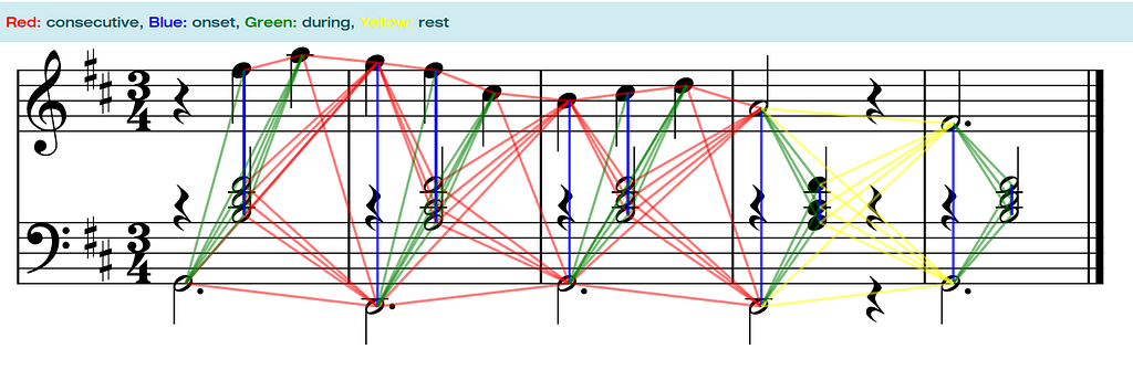
The edges are separated into 4 categories:
This minimal modeling of the graph guarantees that a score will be continuously connected from start to finish without any disconnected subgraphs.
GraphMuse is a Python Library for training and applying deep graph models for music analysis on musical scores.
GraphMuse contains loaders, models, and utils for symbolic music processing with GNNs. It is built on top of PyTorch and PyTorch Geometric for more flexibility and interoperability.
PyTorch is an open-source machine learning library that enables efficient deep learning model building and supports GPU acceleration. PyTorch Geometric is a library built upon PyTorch to easily write and train Graph Neural Networks (GNNs) for a wide range of applications.
Finally, GraphMuse provides functionalities to transform musical scores into graphs. Graph creation is implemented in C code with Python bindings to speedup the graph building, up to x300 faster than the previous numpy-based implementation.
Graphs have been frequently used to analyze and represent music. To cite a few examples, the Tonnetz, Schenkerian analysis, and treelike form analysis are some notable mentions. The advantage of graphs is that they can capture both the hierarchical and the sequential nature of music with the same representation simply by the design of the edges.
Graph-based symbolic music processing using GNNs came about in 2021 with a performance generation model from the score. Since then many graph models have been introduced with some being the state-of-the-art for music analysis tasks up to the date of this post.
So, now that I argued for the necessity of graphs let’s face the complexities of designing and training graph models for symbolic music.
The main complexity of graphs and of course, music is that musical pieces are not always of the same length and the graphs that are created from them are not the same size either. Their size might vary considerably: for example, a Bach chorale might have only 200 notes whereas a Beethoven sonata can have well over 5000. In our graphs, the number of notes corresponds directly to the number of vertices in each score graph.
Training efficiently and fast on score graphs is not a trivial task and would require a sampling method that can maximize the computational resources in terms of both memory and time without deteriorating the performance of the model and sometimes even improving it.
In the training process, sampling involves combining graphs from different scores to create a new graph, often referred to as a “batch” in computer science. Each batch is then fed into the GNN model, where a loss is calculated. This loss is used to backpropagate and update the model’s parameters. This single iteration is called a training step. To optimize the model, this process is repeated many times until the training converges and ideally the model performs optimally.
This all sounds complicated but do not despair because GraphMuse can handle this part for you!!

The general graph processing/training pipeline for symbolic music scores within GraphMuse involves the following steps:
Note that target nodes may include all or a subset of batch nodes depending on the sampling strategy.
Now that the process is graphically explained let’s take a closer look at how GraphMuse handles sampling notes from each score.

Sampling process per score.
To maximize the computational resources (i.e. memory) the above process is repeated for many scores at once to create one batch. Using this process, GraphMuse asserts that every sampled segment is going to have the same size of target notes. Every sampled segment can be combined to a new graph which will be of size at most #_scores x #_target_notes. This new graph constitutes the batch for the current training step.
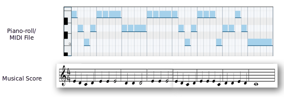
For the hands-on part let’s try to use GraphMuse and use a model for pitch spelling. The pitch spelling task is about inferring the note name and accidentals when they are absent from the score. An example of this application is when we have a quantized midi and want to create a score such as the example in the figure below:
Before installing GraphMuse you will need to install PyTorch and PyTorch Geometric. Check out the appropriate version for your system here and here.
After this step, to install GraphMuse open your preferred terminal and type:
pip install graphmuse
After installation, let’s read a MIDI file from a URL and create the score graph with GraphMuse.
import graphmuse as gm

midi_url_raw = "https://github.com/CPJKU/partitura/raw/refs/heads/main/tests/data/midi/bach_midi_score.mid"
graph = gm.load_midi_to_graph(midi_url_raw)
The underlying process reads the file with Partitura and then feeds it through GraphMuse.
To train our model to handle Pitch Spelling, we first need a dataset of musical scores where the pitch spelling has already been annotated. For this, we’ll be using the ASAP Dataset (licenced under CC BY-NC-SA 4.0), which will serve as the foundation for our model’s learning. To get the ASAP Dataset you can download it using git or directly from github:
git clone https://github.com/cpjku/asap-dataset.git
The ASAP dataset includes scores and performances of various classical piano pieces. For our use-case we will use only the scores which end in .musicxml.
As we load this dataset, we’ll need two essential utilities: one to encode pitch spelling and another to handle key signature information, both of which will be converted into numerical labels. Fortunately, these utilities are available within the pre-built pitch spelling model in GraphMuse. Let’s begin by importing all the necessary packages and loading the first score to get started.
import graphmuse as gm
import partitura as pt
import os
import torch
import numpy as np

# Directory containing the dataset, change this to the location of your dataset
dataset_dir = "/your/path/to/the/asap-dataset"

# Find all the score files in the dataset (they are all named 'xml_score.musicxml')
score_files = [os.path.join(dp, f) for dp, dn, filenames in os.walk(dataset_dir) for f in filenames if f == 'xml_score.musicxml']

# Use the first 30 scores, change this number to use more or less scores
score_files = score_files[:30]

# probe the first score file
score = pt.load_score(score_files[0])
# Extract features and note array
features, f_names = gm.utils.get_score_features(score)
na = score.note_array(include_pitch_spelling=True, include_key_signature=True)
# Create a graph from the score features
graph = gm.create_score_graph(features, score.note_array())

# Get input feature size and metadata from the first graph
in_feats = graph["note"].x.shape[1]
metadata = graph.metadata()

# Create a model for pitch spelling prediction
model = gm.nn.models.PitchSpellingGNN(
    in_feats=in_feats, n_hidden=128, out_feats_enc=64, n_layers=2, metadata=metadata, add_seq=True
)

# Create encoders for pitch and key signature labels
pe = model.pitch_label_encoder
ke = model.key_label_encoder
Next, we’ll load the remaining score files from the dataset to continue preparing our data for model training.
# Initialize lists to store graphs and encoders
graphs = [graph]

# Process each score file
for score_file in score_files[1:]:
    # Load the score
    score = pt.load_score(score_file)

    # Extract features and note array
    features, f_names = gm.utils.get_score_features(score)
    na = score.note_array(include_pitch_spelling=True, include_key_signature=True)

    # Encode pitch and key signature labels
    labels_pitch = pe.encode(na)
    labels_key = ke.encode(na)

    # Create a graph from the score features
    graph = gm.create_score_graph(features, score.note_array())

    # Add encoded labels to the graph
    graph["note"].y_pitch = torch.from_numpy(labels_pitch).long()
    graph["note"].y_key = torch.from_numpy(labels_key).long()

    # Append the graph to the list
    graphs.append(graph)
Once the graph structures are ready, we can move on to creating the data loader, which is conveniently provided by GraphMuse. At this stage, we’ll also define standard training components like the loss function and optimizer to guide the learning process.
# Create a DataLoader to sample subgraphs from the graphs
loader = gm.loader.MuseNeighborLoader(graphs, subgraph_size=100, batch_size=16, num_neighbors=[3, 3])

# Define loss functions for pitch and key prediction
loss_pitch = torch.nn.CrossEntropyLoss()
loss_key = torch.nn.CrossEntropyLoss()

# Define the optimizer
optimizer = torch.optim.Adam(model.parameters(), lr=0.001)
Let me comment a bit more on the gm.loader.MuseNeighborLoader.
This is the core dataloader in GraphMuse and it contains the sampling that was explained in the previous section. subgraph_size refers to the number of target nodes per input graph, batch_size is the number of sampled graphs per batch, and finally, num_neighbors refers to the number of neighbors sampled per sampled node in each layer.
With everything in place, we are finally ready to train the model. So, let’s dive in and start the training process!
# Train the model for 5 epochs
for epoch in range(5):
    loss = 0
    i = 0
    for batch in loader:
        # Zero the gradients
        optimizer.zero_grad()

        # Get neighbor masks for nodes and edges for more efficient training
        neighbor_mask_node = {k: batch[k].neighbor_mask for k in batch.node_types}
        neighbor_mask_edge = {k: batch[k].neighbor_mask for k in batch.edge_types}

        # Forward pass through the model
        pred_pitch, pred_key = model(
            batch.x_dict, batch.edge_index_dict, neighbor_mask_node, neighbor_mask_edge,
            batch["note"].batch[batch["note"].neighbor_mask == 0]
        )

        # Compute loss for pitch and key prediction
        loss_pitch_val = loss_pitch(pred_pitch, batch["note"].y_pitch[batch["note"].neighbor_mask == 0])
        loss_key_val = loss_key(pred_key, batch["note"].y_key[batch["note"].neighbor_mask == 0])

        # Total loss
        loss_val = loss_pitch_val + loss_key_val

        # Backward pass and optimization
        loss_val.backward()
        optimizer.step()

        # Accumulate loss
        loss += loss_val.item()
        i += 1

    # Print average loss for the epoch
    print(f"Epoch {epoch} Loss {loss / i}")
Hopefully, we’ll soon see the loss function decreasing, a positive sign that our model is effectively learning how to perform pitch spelling. Fingers crossed!

GraphMuse is a framework that tries to make the training and deployment of graph models for symbolic music processing easier.
For those who want to retrain, deploy, or finetune previous state-of-the-art models for symbolic music analysis, GraphMuse contains some of the necessary components to re-build and re-train your model faster and more efficiently.
GraphMuse retains its flexibility through its simplicity, for those who want to prototype, innovate, and design new models. It aims to provide a simple set of utilities rather than including complex chained pipelines that can block the innovation process.
For those who want to learn, visualize, and get hands-on experience, GraphMuse is good to get you started. It offers an easy introduction to basic functions and pipelines with a few lines of code. GraphMuse is also linked with MusGViz, which allows graphs and scores to be easily visualized together.
We cannot talk about the positive aspects of any project without discussing the negative ones as well.
GraphMuse is a newborn project and in its current state, it is pretty simple. It is focused on covering the essential parts of graph learning rather than being a holistic framework that covers all possibilities. Therefore it still focuses a lot on user-based implementation on many parts of the aforementioned pipeline.
Like every open-source project in development GraphMuse needs help to grow. So please, if you find bugs or want more features do not hesitate to report, request, or contribute to the GraphMuse GitHub project.
Last but not least, GraphMuse uses C libraries such as torch-sparse and torch-scatter and has its own C-bindings to accelerate graph creation therefore installation is not always straightforward. The windows installation is more challenging judging from our user testing and user interaction reports, although not impossible (I am running it on Windows myself).
Future plans include:
GraphMuse is a Python library that makes working with music graphs a little bit easier. It focuses on the training aspect of graph-based models for music but aims to retain flexibility when research-based projects require it.
If you would like to support the development and future growth of GraphMuse please star the repo here .
Happy graph coding !!!
GitHub – manoskary/graphmuse: A Graph Deep Learning Library for Music.
[all images are by the author]
GraphMuse: A Python Library for Symbolic Music Graph Processing was originally published in Towards Data Science on Medium, where people are continuing the conversation by highlighting and responding to this story.
Originally appeared here:
GraphMuse: A Python Library for Symbolic Music Graph Processing
Go Here to Read this Fast! GraphMuse: A Python Library for Symbolic Music Graph Processing

Large language models (LLMs) have a knowledge cutoff date and cannot answer queries to specific data not present in their knowledge base. For instance, LLMs cannot answer queries about data regarding a company’s meeting minutes from the last year. Similarly, LLMs are prone to hallucinate and provide plausible-looking wrong answers.
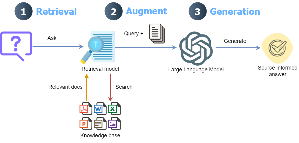
To overcome this issue, Retrieval Augment Generation (RAG) solutions are becoming increasingly popular. The main idea of an RAG is to integrate external documents into LLMs and guide its behavior to answer questions only from the external knowledge base. This is done by chunking the document(s) into smaller chunks, computing each chunk’s embeddings (numerical representations), and storing the embeddings as an index in a specialized vector database.
The process of matching the user’s query with the small chunks in the vector database usually works well; however, it has the following issues:
In response to these issues, Anthropic recently introduced a method to add context to each chunk which showed significant performance improvement over naive RAG. After splitting a document into chunks, this method first assigns a brief context to each chunk by sending the chunk to the LLM along with the entire document as a context. Subsequently, the chunks appended by the context are saved to the vector database. They further combined the contextual chunking with best match using the bm25 retriever that searches documents using the BM25 method, and a re-ranker model that assigns raking scores to each retrieved chunk based on its relevance.
Despite significant performance improvements, Anthropic demonstrated the applicability of these methods only to text. A rich source of information in many documents is images (graphs, figures) and complex tables. If we parse only text from documents, we will not be able to get insights into other modalities in the documents. The documents containing images and complex tables require efficient parsing methods which entails not only properly extracting them from the documents, but also understanding them.
Assigning context to each chunk in the document using Anthropic’s latest model (claude-3–5-sonnet-20240620) could involve high cost in the case of large documents, as it involves sending the whole document with each chunk. Although Claude’s prompt caching technique can significantly reduce this cost by caching frequently used context between API calls, the cost is still much higher than OpenAI’s cost-efficient models such as gpt-4o-mini.
This article discusses an extension of the Anthropic’s methods as follows:
After the Anthropic blog post on contextual retrieval, I found a partial implementation with OpenAI at this GitHub link. However, it uses traditional chunking and LlamaParse without the recently introduced premium mode. I found Llamaparse’s premium mode to be significantly efficient in extracting different structures in the document.
Anthropic’s contextual retrieval implementation can also be found on GitHub which uses LlamaIndex abstraction; however, it does not implement multimodal parsing. At the time of writing this article, a more recent implementation came from LlamaIndex that uses multimodal parsing with contextual retrieval. This implementation uses Anthropic’s LLM (claude-3–5-sonnet-2024062) and Voyage’s embedding model (voyage-3). However, they do not explore best search 25 and re-ranking as mentioned in Anthropic’s blog post.
The contextual retrieval implementation discussed in this article is a low-cost, multimodal RAG solution with improved retrieval performance with BM25 search and re-ranking. The performance of this contextual retrieval-based, multimodal RAG (CMRAG) is also compared with a basic RAG and LlamaIndex’s implementation of contextual retrieval. Some functions were re-used with required modifications from these links: 1, 2, 3, 4.
The code of this implementation is available on GitHub.
The overall approach used in this article to implement the CMRAG is depicted as follows:
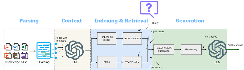
Let’s delve into the step-by-step implementation of CMRAG.
The following libraries need to be installed for running the code discussed in this article.
!pip install llama-index ipython cohere rank-bm25 pydantic nest-asyncio python-dotenv openai llama-parse
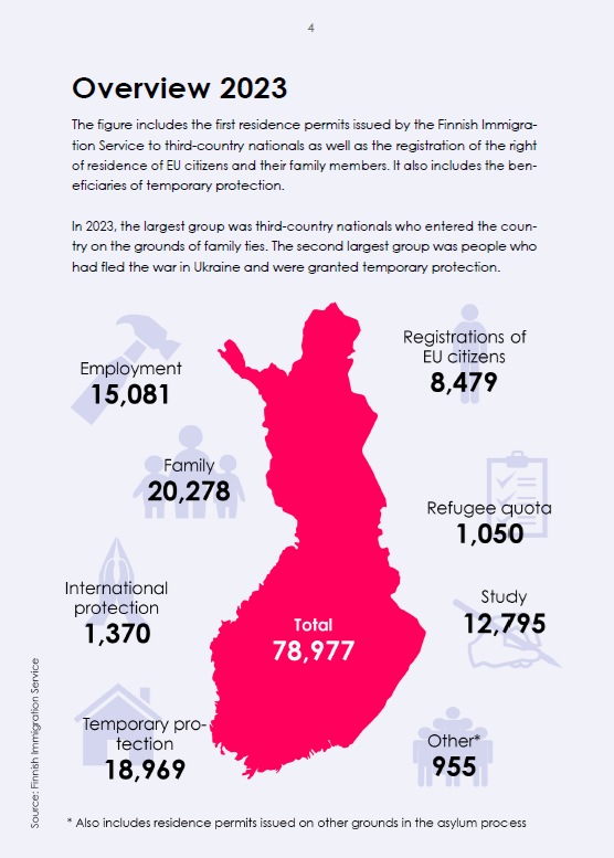
All libraries to be imported to run the whole code are mentioned in the GitHub notebook. For this article, I used Key Figures on Immigration in Finland (licensed under CC By 4.0, re-use allowed) which contains several graphs, images, and text data.
LlamaParse offers multimodal parsing using a vendor multimodal model (such as gpt-4o) to handle document extraction.
parser = LlamaParse(
  use_vendor_multimodal_model=True
  vendor_multimodal_model_name="openai-gpt-4o"
  vendor_multimodal_api_key=sk-proj-xxxxxx
)
In this mode, a screenshot of every page of a document is taken, which is then sent to the multimodal model with instructions to extract as markdown. The markdown result of each page is consolidated into the final output.
The recent LlamaParse Premium mode offers advanced multimodal document parsing, extracting text, tables, and images into well-structured markdown while significantly reducing missing content and hallucinations. It can be used by creating a free account at Llama Cloud Platform and obtaining an API key. The free plan offers to parse 1,000 pages per day.
LlamaParse premium mode is used as follows:
from llama_parse import LlamaParse
import os

# Function to read all files from a specified directory
def read_docs(data_dir) -> List[str]:
    files = []
    for f in os.listdir(data_dir):
        fname = os.path.join(data_dir, f)
        if os.path.isfile(fname):
            files.append(fname)
    return files

parser = LlamaParse(
    result_type="markdown",
    premium_mode=True,
    api_key=os.getenv("LLAMA_CLOUD_API_KEY")
)

files = read_docs(data_dir = DATA_DIR)
We start with reading a document from a specified directory, parse the document using the parser’s get_json_result() method, and get image dictionaries using the parser’s get_images() method. Subsequently, the nodes are extracted and sent to the LLM to assign context based on the overall document using the retrieve_nodes() method. Parsing of this document (60 pages), including getting image dictionaries, took 5 minutes and 34 seconds(a one-time process).
print("Parsing...")
json_results = parser.get_json_result(files)
print("Getting image dictionaries...")
images = parser.get_images(json_results, download_path=image_dir)
print("Retrieving nodes...")
json_results[0]["pages"][3]
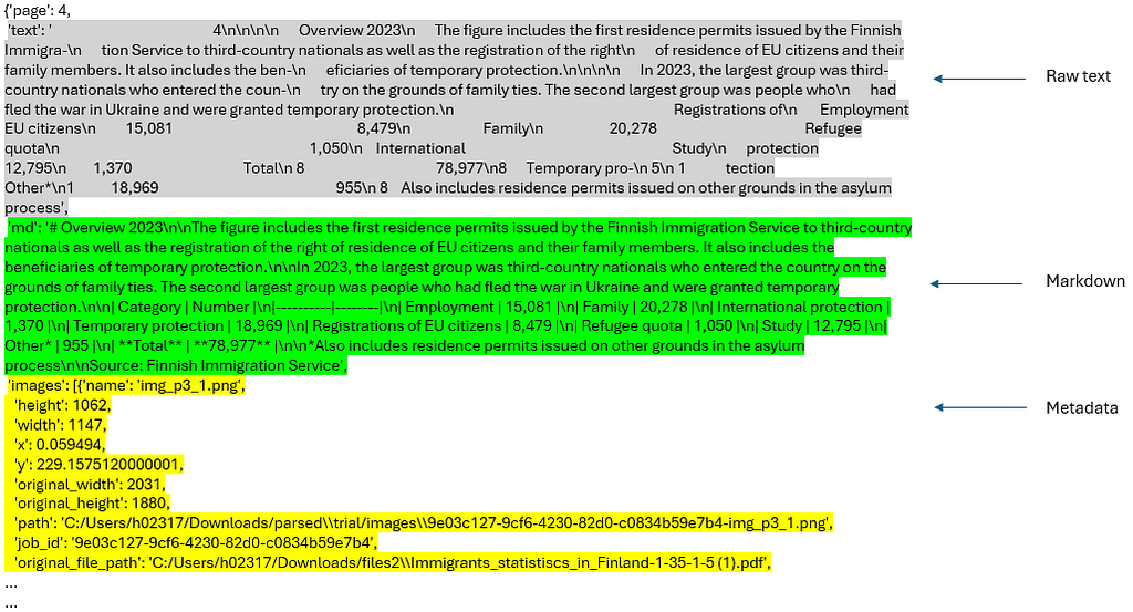
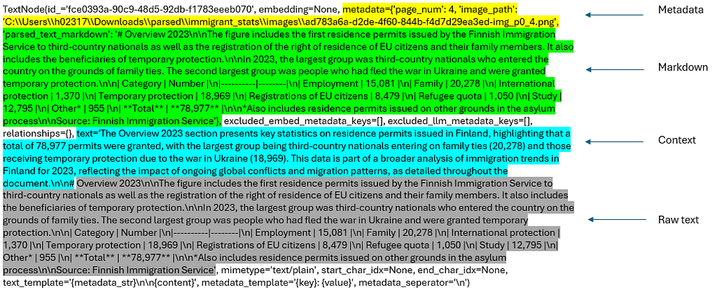
Individual nodes and the associated images (screenshots) are extracted by retrieve_nodes() function from the parsed josn_results. Each node is sent to _assign_context() function along with all the nodes (doc variable in the below code). The _assign_context() function uses a prompt template CONTEXT_PROMPT_TMPL (adopted and modified from this source) to add a concise context to each node. This way, we integrate metadata, markdown text, context, and raw text into the node.
The following code shows the implementation of retrieve_nodes() function. The two helper functions, _get_sorted_image_files() and get_img_page_number(), get sorted image files by page and the page number of images, respectively. The overall aim is not to rely solely on the raw text as the simple RAGs do to generate the final answer, but to consider metadata, markdown text, context, and raw text, as well as the whole images (screenshots) of the retrieved nodes (image links in the node’s metadata) to generate the final response.
# Function to get page number of images using regex on file names
def get_img_page_number(file_name):
    match = re.search(r"-page-(d+).jpg$", str(file_name))
    if match:
        return int(match.group(1))
    return 0

# Function to get image files sorted by page
def _get_sorted_image_files(image_dir):
    raw_files = [f for f in list(Path(image_dir).iterdir()) if f.is_file()]
    sorted_files = sorted(raw_files, key=get_img_page_number)
    return sorted_files

# Context prompt template for contextual chunking
CONTEXT_PROMPT_TMPL = """
You are an AI assistant specializing in document analysis. Your task is to provide brief, relevant context for a chunk of text from the given document.
Here is the document:
<document>
{document}
</document>

Here is the chunk we want to situate within the whole document:
<chunk>
{chunk}
</chunk>

Provide a concise context (2-3 sentences) for this chunk, considering the following guidelines:
1. Identify the main topic or concept discussed in the chunk.
2. Mention any relevant information or comparisons from the broader document context.
3. If applicable, note how this information relates to the overall theme or purpose of the document.
4. Include any key figures, dates, or percentages that provide important context.
5. Do not use phrases like "This chunk discusses" or "This section provides". Instead, directly state the context.

Please give a short succinct context to situate this chunk within the overall document to improve search retrieval of the chunk.
Answer only with the succinct context and nothing else.

Context:
"""

CONTEXT_PROMPT = PromptTemplate(CONTEXT_PROMPT_TMPL)

# Function to generate context for each chunk
def _assign_context(document: str, chunk: str, llm) -> str:
    prompt = CONTEXT_PROMPT.format(document=document, chunk=chunk)
    response = llm.complete(prompt)
    context = response.text.strip()
    return context

# Function to create text nodes with context
def retrieve_nodes(json_results, image_dir, llm) -> List[TextNode]:
    nodes = []
    for result in json_results:
        json_dicts = result["pages"]
        document_name = result["file_path"].split('/')[-1]
        docs = [doc["md"] for doc in json_dicts]  # Extract text
        image_files = _get_sorted_image_files(image_dir)  # Extract images
        # Join all docs to create the full document text
        document_text = "nn".join(docs)
        for idx, doc in enumerate(docs):
            # Generate context for each chunk (page)
            context = _assign_context(document_text, doc, llm)
            # Combine context with the original chunk
            contextualized_content = f"{context}nn{doc}"
            # Create the text node with the contextualized content
            chunk_metadata = {"page_num": idx + 1}
            chunk_metadata["image_path"] = str(image_files[idx])
            chunk_metadata["parsed_text_markdown"] = docs[idx]

            node = TextNode(
                text=contextualized_content,
                metadata=chunk_metadata,
            )
            nodes.append(node)
    return nodes
# Get text nodes
text_node_with_context = retrieve_nodes(json_results, image_dir, llm)First page of the report (image by author)First page of the report (image by author)
Here is the depiction of a node corresponding to the first page of the report.
All the nodes with metadata, raw text, markdown text, and context information are then indexed into a vector database. BM25 indices for the nodes are created and saved in a pickle file for query inference. The processed nodes are also saved for later use (text_node_with_context.pkl).
    # Create the vector store index
    index = VectorStoreIndex(text_node_with_context, embed_model=embed_model)
    index.storage_context.persist(persist_dir=output_dir)
    # Build BM25 index
    documents = [node.text for node in text_node_with_context]
    tokenized_documents = [doc.split() for doc in documents]
    bm25 = BM25Okapi(tokenized_documents)
    # Save bm25 and text_node_with_context
    with open(os.path.join(output_dir, 'tokenized_documents.pkl'), 'wb') as f:
        pickle.dump(tokenized_documents, f)
    with open(os.path.join(output_dir, 'text_node_with_context.pkl'), 'wb') as f:
        pickle.dump(text_node_with_context, f)
We can now initialize a query engine to ask queries using the following pipeline. But before that, the following prompt is set to guide the behavior of the LLM to generate the final response. A multimodal LLM (gpt-4o-mini) is initialized to generate the final response. This prompt can be adjusted as needed.
# Define the QA prompt template
RAG_PROMPT = """
Below we give parsed text from documents in two different formats, as well as the image.

---------------------
{context_str}
---------------------
Given the context information and not prior knowledge, answer the query. Generate the answer by analyzing parsed markdown, raw text and the related
image. Especially, carefully analyze the images to look for the required information.
Format the answer in proper format as deems suitable (bulleted lists, sections/sub-sections, tables, etc.)
Give the page's number and the document name where you find the response based on the Context.

Query: {query_str}
Answer: """

PROMPT = PromptTemplate(RAG_PROMPT)

# Initialize the multimodal LLM
MM_LLM = OpenAIMultiModal(model="gpt-4o-mini", temperature=0.0, max_tokens=16000)
The following QueryEngine class implements the above-mentioned workflow. The number of nodes in BM25 search (top_n_bm25) and the number of re-ranked results (top_n) by the re-ranker can be adjusted as required. The BM25 search and re-ranking can be selected or de-selected by toggling the best_match_25 and re_ranking variables in the GitHub code.
Here is the overall workflow implemented by QueryEngine class.
# DeFfine the QueryEngine integrating all methods
class QueryEngine(CustomQueryEngine):
    # Public fields
    qa_prompt: PromptTemplate
    multi_modal_llm: OpenAIMultiModal
    node_postprocessors: Optional[List[BaseNodePostprocessor]] = None

    # Private attributes using PrivateAttr
    _bm25: BM25Okapi = PrivateAttr()
    _llm: OpenAI = PrivateAttr()
    _text_node_with_context: List[TextNode] = PrivateAttr()
    _vector_index: VectorStoreIndex = PrivateAttr()

    def __init__(
        self,
        qa_prompt: PromptTemplate,
        bm25: BM25Okapi,
        multi_modal_llm: OpenAIMultiModal,
        vector_index: VectorStoreIndex,
        node_postprocessors: Optional[List[BaseNodePostprocessor]] = None,
        llm: OpenAI = None,
        text_node_with_context: List[TextNode] = None,
    ):
        super().__init__(
            qa_prompt=qa_prompt,
            retriever=None,
            multi_modal_llm=multi_modal_llm,
            node_postprocessors=node_postprocessors
        )
        self._bm25 = bm25
        self._llm = llm
        self._text_node_with_context = text_node_with_context
        self._vector_index = vector_index

    def custom_query(self, query_str: str):
        # Prepare the query bundle
        query_bundle = QueryBundle(query_str)

        bm25_nodes = []
        if best_match_25 == 1:  # if BM25 search is selected
            # Retrieve nodes using BM25
            query_tokens = query_str.split()
            bm25_scores = self._bm25.get_scores(query_tokens)
            top_n_bm25 = 5  # Adjust the number of top nodes to retrieve
            # Get indices of top BM25 scores
            top_indices_bm25 = bm25_scores.argsort()[-top_n_bm25:][::-1]
            bm25_nodes = [self._text_node_with_context[i] for i in top_indices_bm25]
            logging.info(f"BM25 nodes retrieved: {len(bm25_nodes)}")
        else:
            logging.info("BM25 not selected.")

        # Retrieve nodes using vector-based retrieval from the vector store
        vector_retriever = self._vector_index.as_query_engine().retriever
        vector_nodes_with_scores = vector_retriever.retrieve(query_bundle)
        # Specify the number of top vectors you want
        top_n_vectors = 5  # Adjust this value as needed
        # Get only the top 'n' nodes
        top_vector_nodes_with_scores = vector_nodes_with_scores[:top_n_vectors]
        vector_nodes = [node.node for node in top_vector_nodes_with_scores]
        logging.info(f"Vector nodes retrieved: {len(vector_nodes)}")

        # Combine nodes and remove duplicates
        all_nodes = vector_nodes + bm25_nodes
        unique_nodes_dict = {node.node_id: node for node in all_nodes}
        unique_nodes = list(unique_nodes_dict.values())
        logging.info(f"Unique nodes after deduplication: {len(unique_nodes)}")

        nodes = unique_nodes

        if re_ranking == 1:  # if re-ranking is selected
            # Apply Cohere Re-ranking to rerank the combined results
            documents = [node.get_content() for node in nodes]
            max_retries = 3
            for attempt in range(max_retries):
                try:
                    reranked = cohere_client.rerank(
                        model="rerank-english-v2.0",
                        query=query_str,
                        documents=documents,
                        top_n=3  # top-3 re-ranked nodes
                    )
                    break
                except CohereError as e:
                    if attempt < max_retries - 1:
                        logging.warning(f"Error occurred: {str(e)}. Waiting for 60 seconds before retry {attempt + 1}/{max_retries}")
                        time.sleep(60)  # Wait before retrying
                    else:
                        logging.error("Error occurred. Max retries reached. Proceeding without re-ranking.")
                        reranked = None
                        break

            if reranked:
                reranked_indices = [result.index for result in reranked.results]
                nodes = [nodes[i] for i in reranked_indices]
            else:
                nodes = nodes[:3]  # Fallback to top 3 nodes
            logging.info(f"Nodes after re-ranking: {len(nodes)}")
        else:
            logging.info("Re-ranking not selected.")

        # Limit and filter node content for context string
        max_context_length = 16000  # Adjust as required
        current_length = 0
        filtered_nodes = []

        # Initialize tokenizer
        from transformers import GPT2TokenizerFast
        tokenizer = GPT2TokenizerFast.from_pretrained("gpt2")

        for node in nodes:
            content = node.get_content(metadata_mode=MetadataMode.LLM).strip()
            node_length = len(tokenizer.encode(content))
            logging.info(f"Node ID: {node.node_id}, Content Length (tokens): {node_length}")
            if not content:
                logging.warning(f"Node ID: {node.node_id} has empty content. Skipping.")
                continue
            if current_length + node_length <= max_context_length:
                filtered_nodes.append(node)
                current_length += node_length
            else:
                logging.info(f"Reached max context length with Node ID: {node.node_id}")
                break
        logging.info(f"Filtered nodes for context: {len(filtered_nodes)}")

        # Create context string
        ctx_str = "nn".join(
            [n.get_content(metadata_mode=MetadataMode.LLM).strip() for n in filtered_nodes]
        )

        # Create image nodes from the images associated with the nodes
        image_nodes = []
        for n in filtered_nodes:
            if "image_path" in n.metadata:
                image_nodes.append(
                    NodeWithScore(node=ImageNode(image_path=n.metadata["image_path"]))
                )
            else:
                logging.warning(f"Node ID: {n.node_id} lacks 'image_path' metadata.")
        logging.info(f"Image nodes created: {len(image_nodes)}")

        # Prepare prompt for the LLM
        fmt_prompt = self.qa_prompt.format(context_str=ctx_str, query_str=query_str)

        # Use the multimodal LLM to interpret images and generate a response
        llm_response = self.multi_modal_llm.complete(
            prompt=fmt_prompt,
            image_documents=[image_node.node for image_node in image_nodes],
            max_tokens=16000
        )

        logging.info(f"LLM response generated.")

        # Return the final response
        return Response(
            response=str(llm_response),
            source_nodes=filtered_nodes,
            metadata={
                "text_node_with_context": self._text_node_with_context,
                "image_nodes": image_nodes,
            },
        )

# Initialize the query engine with BM25, Cohere Re-ranking, and Query Expansion
query_engine = QueryEngine(
    qa_prompt=PROMPT,
    bm25=bm25,
    multi_modal_llm=MM_LLM,
    vector_index=index,
    node_postprocessors=[],
    llm=llm,
    text_node_with_context=text_node_with_context
)
print("All done")
An advantage of using OpenAI models, especially gpt-4o-mini, is much lower cost for context assignment and query inference running, as well as much smaller context assignment time. While the basic tiers of both OpenAI and Anthropic do quickly hit the maximum rate limit of API calls, retry time in Anthropic’s basic tier vary and could be too long. Context assignment process for only first 20 pages of this document with claude-3–5-sonnet-20240620 took approximately 170 seconds with prompt caching and costed 20 cents (input + output tokens). Whereas, gpt-4o-mini is roughly 20x cheaper compared to Claude 3.5 Sonnet for input tokens and roughly 25x cheaper for output tokens. OpenAI claims to implement prompt caching for repetitive content which works automatically for all API calls.
In comparison, the context assignment to nodes in this entire document (60 pages) through gpt-4o-mini completed in approximately 193 seconds without any retry request.
After implementing the QueryEngine class, we can run the query inference as follows:
original_query = """What are the top countries to whose citizens the Finnish Immigration Service issued the highest number of first residence permits in 2023?
Which of these countries received the highest number of first residence permits?"""
response = query_engine.query(original_query)
display(Markdown(str(response)))
Here is the markdown response to this query.

The pages cited in the query response are the following.

Now let’s compare the performance of gpt-4o-mini based RAG (LlamaParse premium + context retrieval + BM25 + re-ranking) with Claude based RAG (LlamaParse premium + context retrieval). I also implemented a simple, baseline RAG which can be found in GitHub’s notebook. Here are the three RAGs to be compared.
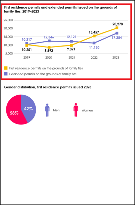
For the sake of simplicity, we refer to these RAGs as RAG0, RAG1, and RAG2, respectively. Here are three pages from the report from where I asked three questions (1 question from each page) to each RAG. The areas highlighted by the red rectangles show the ground truth or the place from where the right answer should come from.


Here are the responses to the three RAGs to each question.
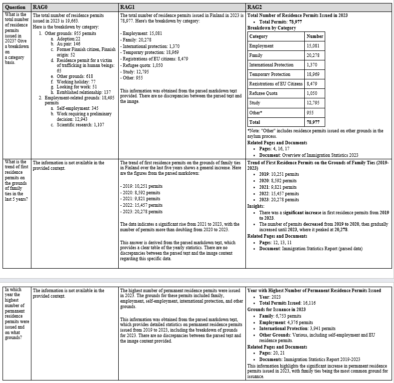
It can be seen that RAG2 performs very well. For the first question, RAG0 provides a wrong answer because the question was asked from an image. Both RAG1 and RAG2 provided the right answer to this question. For the other two questions, RAG0 could not provide any answer. Whereas, both RAG1 and RAG2, provided right answers to these questions.
Overall, RAG2’s performance was equal or even better than RAG1 in many cases due to the integration of BM25, re-ranking, and better prompting. It provides a cost-effective solution to a contextual, multimodal RAG. A possible integration in this pipeline could be hypothetical document embedding (hyde) or query extension. Similarly, open-source embedding models (such as all-MiniLM-L6-v2) and/or light-weight LLMs (such as gemma2 or phi-3-small) could also be explored to make it more cost effective.
If you like the article, please clap the article and follow me on Medium and/or LinkedIn
For the full code reference, please take a look at my repo:
GitHub – umairalipathan1980/Multimodal-contextual-RAG: Multimodal contextual RAG
Integrating Multimodal Data into a Large Language Model was originally published in Towards Data Science on Medium, where people are continuing the conversation by highlighting and responding to this story.
Originally appeared here:
Integrating Multimodal Data into a Large Language Model
Go Here to Read this Fast! Integrating Multimodal Data into a Large Language Model
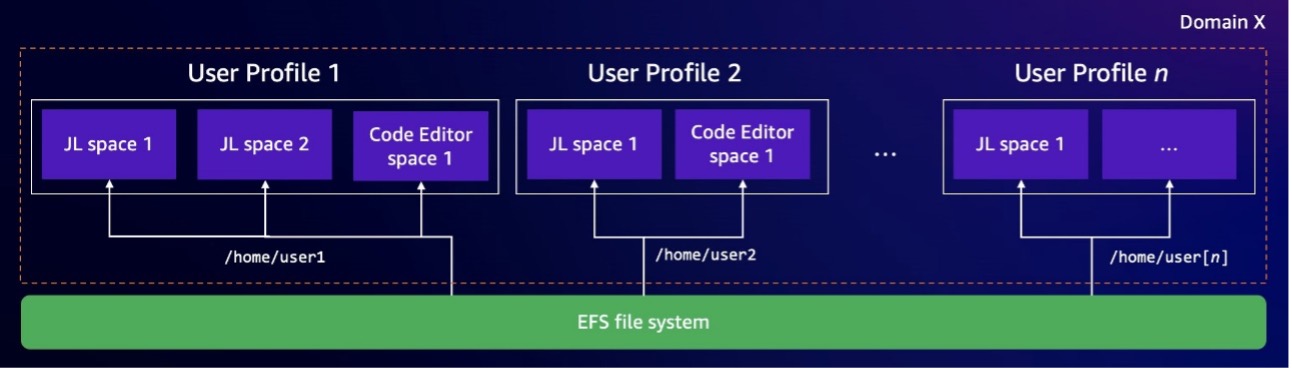

Originally appeared here:
Use Amazon SageMaker Studio with a custom file system in Amazon EFS
Go Here to Read this Fast! Use Amazon SageMaker Studio with a custom file system in Amazon EFS

Originally appeared here:
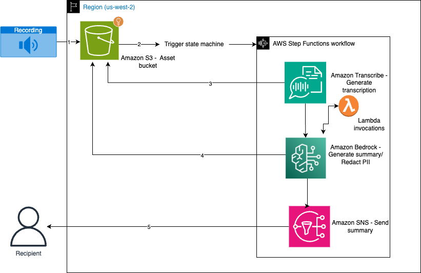
Summarize call transcriptions securely with Amazon Transcribe and Amazon Bedrock Guardrails
Feeling inspired to write your first TDS post? We’re always open to contributions from new authors.
Whether you’re fresh out of your degree or bootcamp, or looking to transition into a data science role from a different field, the various paths towards landing your first (or second, or third) job cross an ever-shifting terrain. The necessary skill sets continue to evolve, new tools and technologies pop up on a daily basis, and the job market itself has become more competitive in recent years. What’s an aspiring data scientist to do?
Well, a good first step would be to read this week’s highlights, which tackle these perennial questions with up-to-date insights and actionable advice. From finding your footing as a freelancer to ensuring you successfully market your existing knowledge and experience, these articles offer concrete roadmaps grounded in their authors’ own professional journeys. Enjoy your reading!
Ready to expand your horizons beyond the current job market and its challenges? We hope so—here are some of our best recent articles, on topics ranging from the 2024 Physics Nobel Prize to partitioning algorithms and AI product development.
Thank you for supporting the work of our authors! As we mentioned above, we love publishing articles from new authors, so if you’ve recently written an interesting project walkthrough, tutorial, or theoretical reflection on any of our core topics, don’t hesitate to share it with us.
Until the next Variable,
TDS Team
What Does It Take to Get Your Foot in the Door as a Data Scientist? was originally published in Towards Data Science on Medium, where people are continuing the conversation by highlighting and responding to this story.
Originally appeared here:
What Does It Take to Get Your Foot in the Door as a Data Scientist?
Go Here to Read this Fast! What Does It Take to Get Your Foot in the Door as a Data Scientist?

I recently had the opportunity to provide analysis on an interesting project, and I had more to say than could be included in that single piece, so today I’m going to discuss some more of my thoughts about it.
The approach the researchers took with this project involved providing a series of prompts to different generative AI image generation tools: Stable Diffusion, Midjourney, YandexART, and ERNIE-ViLG (by Baidu). The prompts were particularly framed around different generations — Baby Boomers, Gen X, Millennials, and Gen Z, and requested images of these groups in different contexts, such as “with family”, “on vacation”, or “at work”.
While the results were very interesting, and perhaps revealed some insights about visual representation, I think we should also take note of what this cannot tell us, or what the limitations are. I’m going to divide up my discussion into the aesthetics (what the pictures look like) and representation (what is actually shown in the images), with a few side tracks into how these images come to exist in the first place, because that’s really important to both topics.
Before I start, though, a quick overview of these image generator models. They’re created by taking giant datasets of images (photographs, artwork, etc) paired with short text descriptions, and the goal is to get the model to learn the relationships between words and the appearance of the images, such that when given a word the model can create an image that matches, more or less. There’s a lot more detail under the hood, and the models (like other generative AI) have a built in degree of randomness that allows for variations and surprises.
When you use one of these hosted models, you give a text prompt and an image is returned. However, it’s important to note that your prompt is not the ONLY thing the model gets. There are also built in instructions, which I call pre-prompting instructions sometimes, and these can have an effect on what the output is. Examples might be telling the model to refuse to create certain kinds of offensive images, or to reject prompts using offensive language.
An important framing point here is that the training data, those big sets of images that are paired with text blurbs, is what the model is trying to replicate. So, we should ask more questions about the training data, and where it comes from. To train models like these, the volume of image data required is extraordinary. Midjourney was trained on https://laion.ai/, whose larger dataset has 5 billion image-text pairs across multiple languages, and we can assume the other models had similar volumes of content. This means that engineers can’t be TOO picky about which images are used for training, because they basically need everything they can get their hands on.
Ok, so where do we get images? How are they generated? Well, we create our own and post them on social media by the bucketload, so that’s necessarily going to be a chunk of it. (It’s also easy to get a hold of, from these platforms.) Media and advertising also create tons of images, from movies to commercials to magazines and beyond. Many other images are never going to be accessible to these models, like your grandma’s photo album that no one has digitized, but the ones that are available to train are largely from these two buckets: independent/individual creators and media/ads.
So, what do you actually get when you use one of these models?
One thing you’ll notice if you try out these different image generators is the stylistic distinctions between them, and the internal consistency of styles. I think this is really fascinating, because they feel like they almost have personalities! Midjourney is dark and moody, with shadowy elements, while Stable Diffusion is bright and hyper-saturated, with very high contrast. ERNIE-ViLG seems to lean towards a cartoonish style, also with very high contrast and textures appearing rubbery or highly filtered. YandexART has washed out coloring, with often featureless or very blurred backgrounds and the appearance of spotlighting (it reminds me of a family photo taken at a department store in some cases). A number of different elements may be responsible for each model’s trademark style.
As I’ve mentioned, pre-prompting instructions are applied in addition to whatever input the user gives. These may indicate specific aesthetic components that the outputs should always have, such as stylistic choices like the color tones, brightness, and contrast, or they may instruct the model not to follow objectionable instructions, among other things. This forms a way for the model provider to implement some limits and guardrails on the tool, preventing abuse, but can also create aesthetic continuity.
The process of fine tuning with reinforcement learning may also affect style, where human observers are making judgments about the outputs that are provided back to the model for learning. The human observers will have been trained and given instructions about what kinds of features of the output images to approve of/accept and which kinds should be rejected or down-scored, and this may involve giving higher ratings to certain kinds of visuals.
The type of training data also has an impact. We know some of the massive datasets that are employed for training the models, but there is probably more we don’t know, so we have to infer from what the models produce. If the model is producing high-contrast, brightly colored images, there’s a good chance the training data included a lot of images with those characteristics.
As we analyze the outputs of the different models, however, it’s important to keep in mind that these styles are probably a combination of pre-prompting instructions, the training data, and the human fine tuning.
Beyond the visual appeal/style of the images, what’s actually in them?
What the models will have the capability to do is going to be limited by the reality of how they’re trained. These models are trained on images from the past — some the very recent past, but some much further back. For example, consider: as we move forward in time, younger generations will have images of their entire lives online, but for older groups, images from their youth or young adulthood are not available digitally in large quantities (or high quality) for training data, so we may never see them presented by these models as young people. It’s very visible in this project: For Gen Z and Millennials, in this data we see that the models struggle to “age” the subjects in the output appropriately to the actual age ranges of the generation today. Both groups seem to look more or less the same age in most cases, with Gen Z sometimes shown (in prompts related to schooling, for example) as actual children. In contrast, Boomers and Gen X are shown primarily in middle age or old age, because the training data that exists is unlikely to have scanned copies of photographs from their younger years, from the 1960s-1990s. This makes perfect sense if you think in the context of the training data.
[A]s we move forward in time, younger generations will have images of their entire lives online, but for older groups, images from their youth or young adulthood are not available digitally for training data, so we may never see them presented by these models as young people.
With this in mind, I’d argue that what we can get from these images, if we investigate them, is some impression of A. how different age groups present themselves in imagery, particularly selfies for the younger sets, and B. how media representation looks for these groups. (It’s hard to break these apart sometimes, because media and youth culture are so dialectical.)
The training data didn’t come out of nowhere — human beings chose to create, share, label, and curate the images, so those people’s choices are coloring everything about them. The models are getting the image of these generations that someone has chosen to portray, and in all cases these portrayals have a reason and intention behind it.
A teen or twentysomething taking a selfie and posting it online (so that it is accessible to become training data for these models) probably took ten, or twenty, or fifty before choosing which one to post to Instagram. At the same time, a professional photographer choosing a model to shoot for an ad campaign has many considerations in play, including the product, the audience, the brand identity, and more. Because professional advertising isn’t free of racism, sexism, ageism, or any of the other -isms, these images won’t be either, and as a result, the image output of these models comes with that same baggage. Looking at the images, you can see many more phenotypes resembling people of color among Millennial and Gen Z for certain models (Midjourney and Yandex in particular), but hardly any of those phenotypes among Gen X and Boomers in the same models. This may be at least partly because advertisers targeting certain groups choose representation of race and ethnicity (as well as age) among models that they believe will appeal to them and be relatable, and they’re presupposing that Boomers and Gen X are more likely to purchase if the models are older and white. These are the images that get created, and then end up in the training data, so that’s what the models learn to produce.
The point I want to make is that these are not free of influence from culture and society — whether that influence is good or bad. The training data came from human creations, so the model is bringing along all the social baggage that those humans had.
The point I want to make is that these are not free of influence from culture and society — whether that influence is good or bad. The training data came from human creations, so the model is bringing along all the social baggage that those humans had.
Because of this reality, I think that asking whether we can learn about generations from the images that models produce is kind of the wrong question, or at least a misguided premise. We might incidentally learn something about the people whose creations are in the training set, which may include selfies, but we’re much more likely to learn about the broader society, in the form of people taking pictures of others as well as themselves, the media, and commercialism. Some (or even a lot) of what we’re getting, especially for the older groups who don’t contribute as much self-generated visual media online, is at best perceptions of that group from advertising and media, which we know has inherent flaws.
Is there anything to be gained about generational understanding from these images? Perhaps. I’d say that this project can potentially help us see how generational identities are being filtered through media, although I wonder if it is the most convenient or easy way to do that analysis. After all, we could go to the source — although the aggregation that these models conduct may be academically interesting. It also may be more useful for younger generations, because more of the training data is self-produced, but even then I still think we should remember that we imbue our own biases and agendas into the images we put out into the world about ourselves.
As an aside, there is a knee-jerk impulse among some commentators to demand some sort of whitewashing of the things that models like this create— that’s how we get models that will create images of Nazi soldiers of various racial and ethnic appearances. As I’ve written before, this is largely a way to avoid dealing with the realities about our society that models feed back to us. We don’t like the way the mirror looks, so we paint over the glass instead of considering our own face.
Of course, that’s not completely true either — all of our norms and culture are not going to be represented in the model’s output, only that which we commit to images and feed in to the training data. We’re seeing some slice of our society, but not the whole thing in a truly warts-and-all fashion. So, we must set our expectations realistically based on what these models are and how they are created. We are not getting a pristine picture of our lives in these models, because the photos we take (and the ones we don’t take, or don’t share), and the images media creates and disseminates, are not free of bias or objective. It’s the same reason we shouldn’t judge ourselves and our lives against the images our friends post on Instagram — that’s not a complete and accurate picture of their life either. Unless we implement a massive campaign of photography and image labeling that pursues accuracy and equal representation, for use in training data, we are not going to be able to change the way this system works.
Getting to spend time with these ideas has been really interesting for me, and I hope the analysis is helpful for those of you who use these kinds of models regularly. There are lots of issues with using generative AI image generating models, from the environmental to the economic, but I think understanding what they are (and aren’t) and what they really do is critical if you choose to use the models in your day to day.
Read more from me at www.stephaniekirmer.com.
https://www.theverge.com/2024/2/21/24079371/google-ai-gemini-generative-inaccurate-historical
The project: https://bit.ly/genaiSK
A Critical Look at AI Image Generation was originally published in Towards Data Science on Medium, where people are continuing the conversation by highlighting and responding to this story.
Originally appeared here:
A Critical Look at AI Image Generation
Go Here to Read this Fast! A Critical Look at AI Image Generation