In this post, we learn how SnapLogic’s Agent Creator leverages Amazon Bedrock to provide a low-code platform that enables enterprises to quickly develop and deploy powerful generative AI applications without deep technical expertise.
In this post, we discuss how Classworks uses Amazon Bedrock and Anthropic’s Claude Sonnet to deliver next-generation differentiated learning with Wittly.
In this post, we demonstrate how to use Amazon Bedrock to create synthetic data, fine-tune a BAAI General Embeddings (BGE) model, and deploy it using Amazon SageMaker.
In this post, we show you how to unlock powerful post-call analytics and visualizations, empowering your organization to make data-driven decisions and drive continuous improvement.
In this post, we demonstrate how to deploy a contextual AI assistant. We build a solution which provides users with a familiar and convenient interface using Amazon Bedrock Knowledge Bases, Amazon Lex, and Amazon Connect, with WhatsApp as the channel.
When developing a machine learning project in an industry, data scientists and ML engineers are often the primary roles highlighted. However, in reality, it takes a village to deliver the product. In a previous article, we discussed the steps involved in developing a fraud prediction product using machine learning. In this article, we will explore the various roles in such a project and how each contributes to its success. Disclaimer: Not all projects will necessarily have teams or individuals with the exact titles listed below; depending on the company structure, one person may wear multiple hats and fulfill several roles. Here, I outline the structure based on my experience of working on different fraud prediction projects with ML/AI.
Project Manager
The project manager’s role is both critical and challenging. They are responsible for the project’s plan and its execution. At the beginning of the project, they help define the plan and set deadlines based on stakeholders’ requests and the technical team’s capacities. Throughout the project, they constantly monitor progress. If the actual state of tasks or deliveries deviates from the plan, they need to raise a flag and coordinate with the teams. As a result, they spend most of their time communicating with different teams, higher-level managers, and business stakeholders. Two major challenges in their job are:
Interdependency between Technical Teams: This makes the role challenging because the outputs from one team (e.g., data engineers ingesting the data) serve as inputs to another team (e.g., data scientists consuming the data). Any delay or change in the first step impacts the second step. Project managers, though not typically super technical, need to be aware of these changes and ensure proper communication between teams.
Competing Business Priorities: Business stakeholders often change their priorities, or there may be competing priorities across different teams that need to be aligned. Project managers must navigate these changes and align the various teams to keep the project on track.
By effectively managing these challenges, project managers play a pivotal role in the successful delivery of machine learning projects.
Fraud analyst
Fraud analysts’ domain expertise and knowledge are crucial for the development and evaluation of fraud prediction models. From the beginning of the project, they provide insights into active fraud trends, common fraudulent scenarios, and red flags, as well as exceptions or “green flags.” Data scientists incorporate this knowledge during the feature creation/engineering phase. Once the model is running in production, constant monitoring is required to maintain or improve performance. At this stage, fraud analysts are essential in identifying the model’s true or false positives. This identification can result from a thorough investigation of the customer’s history or by contacting the customer for confirmation. The feedback from fraud analysts is integral to the feedback loop process.
High level management (chief officers of compliance, strategy, marketing, etc.)
High-level managers and C-level executives play a crucial role in the success of ML/AI fraud projects. Their support is essential for removing obstacles and building consensus on the project’s strategic direction. Therefore, they need to be regularly updated about the project’s progress. So that they can support championing investments in necessary teams, tools, and processes based on the project’s specific requirements and ensure appropriate resources are allocated. Additionally, they are responsible for holding internal and external parties accountable for data privacy and compliance with industry standards. By fostering a culture of accountability and providing clear leadership, they help ensure that the project meets its goals and integrates smoothly with the organization’s overall strategy. Their involvement is vital for addressing any regulatory concerns, managing risk, and driving the project toward successful implementation and long-term sustainability.
Data Engineers
Data engineers provide the data needed for us (data scientists) to build models, which is an essential step in any ML project. They are responsible for designing and maintaining data pipelines, whether for real-time data streams or batch processes in data warehouses. Involved from the project’s inception, data engineers identify data requirements, sources, processing needs, and SLA requirements for data accessibility.
They build pipelines to collect, transform, and store data from various sources, essentially handling the ETL process. They also manage and maintain these pipelines, addressing scalability requirements, monitoring data quality, optimizing queries and processes to improve latency, and reducing costs.
Data scientists
On paper, data scientists create machine learning algorithms to predict various types of information for the business. In reality, we wear many different hats throughout the day. We start by identifying the business problem, understanding the data and available resources, and defining a solution, translating it into technical requirements.
Data scientists collaborate closely with data engineers and MLOps engineers to implement solutions. We also work with business stakeholders to communicate results and receive feedback. Model evaluation is another critical responsibility, which involves selecting proper metrics to assess the model’s performance, continuously monitoring and reporting on it, and watching for any decay in performance.
The process of continuous improvement is central to a data scientist’s role, to ensure that models remain accurate and relevant over time.
Mlops Engineers
Once data engineers and data scientists build the data pipelines and model, it’s time to put the model into production. MLOps engineers play a crucial role in this phase by bridging the gap between development and operations. In the context of fraud prediction, timing is critical since the business needs to prevent fraud before it happens, necessitating a pipeline process that runs in less than a second. Therefore, Mlops engineers ensure that models are seamlessly integrated into production environments, maintaining reliability and scalability. MLOps engineers design and manage the infrastructure needed for model deployment, implement continuous integration and continuous deployment (CI/CD) pipelines, and monitor model performance in real-time. They also handle version control, automate testing, and manage model retraining processes to keep models up-to-date. By addressing these operational challenges, MLOps engineers enable the smooth and efficient deployment of machine learning models, ensuring they deliver consistent and valuable outcomes for the business.
Last word!
We talked about the roles I have identified in my working experience. These roles interact differently depending on the stage of the project and each specific company. In my experience, in the begining of the project, fraud analysts, high level managers and data scientists work together to define the strategy and requirements. Data scientist’s play a significant role in identifying the business problem. They collaborate with Mlops and Engineering to translate it into a technical solution. Data engineers need to come along to discuss required pipeline developments. One common challenge is when there is a disconnect between these teams and it just emerges at the time of execution. This can impact timelines and the quality of the deliverable. Therefore the more integrity between these teams, the smoother will be the implementation and delivery.
Comment below about the roles in your company. How are things different in your experience?
The universal principle of knowledge distillation, model compression, and rule extraction
Figure 1. This and other images were created by the author with the help of recraft.ai
Machine learning (ML) model training typically follows a familiar pipeline: start with data collection, clean and prepare it, then move on to model fitting. But what if we could take this process further? Just as some insects undergo dramatic transformations before reaching maturity, ML models can evolve in a similar way (see Hinton et al. [1]) — what I will call the ML metamorphosis. This process involves chaining different models together, resulting in a final model that achieves significantly better quality than if it had been trained directly from the start.
Here’s how it works:
Start with some initial knowledge, Data 1.
Train an ML model, Model A (say, a neural network), on this data.
Generate new data, Data 2, using Model A.
Finally, use Data 2 to fit your target model, Model B.
Figure 2. An illustration of the ML metamorphosis
You may already be familiar with this concept from knowledge distillation, where a smaller neural network replaces a larger one. But ML metamorphosis goes beyond this, and neither the initial model (Model A) nor the final one (Model B) need be neural networks at all.
Example: ML metamorphosis on the MNIST Dataset
Imagine you’re tasked with training a multi-class decision tree on the MNIST dataset of handwritten digit images, but only 1,000 images are labelled. You could train the tree directly on this limited data, but the accuracy would be capped at around 0.67. Not great, right? Alternatively, you could use ML metamorphosis to improve your results.
But before we dive into the solution, let’s take a quick look at the techniques and research behind this approach.
1. Knowledge distillation (2015)
Even if you haven’t used knowledge distillation, you’ve probably seen it in action. For example, Meta suggests distilling its Llama 3.2 model to adapt it to specific tasks [2]. Or take DistilBERT — a distilled version of BERT [3]— or the DMD framework, which distills Stable Diffusion to speed up image generation by a factor of 30 [4].
At its core, knowledge distillation transfers knowledge from a large, complex model (the teacher) to a smaller, more efficient model (the student). The process involves creating a transfer set that includes both the original training data and additional data (either original or synthesized) pseudo-labeled by the teacher model. The pseudo-labels are known as soft labels — derived from the probabilities predicted by the teacher across multiple classes. These soft labels provide richer information than hard labels (simple class indicators) because they reflect the teacher’s confidence and capture subtle similarities between classes. For instance, they might show that a particular “1” is more similar to a “7” than to a “5.”
By training on this enriched transfer set, the student model can effectively mimic the teacher’s performance while being much lighter, faster, and easier to use.
The student model obtained in this way is more accurate than it would have been if it had been trained solely on the original training set.
2. Model compression (2007)
Model compression [5] is often seen as a precursor to knowledge distillation, but there are important differences. Unlike knowledge distillation, model compression doesn’t seem to use soft labels, despite some claims in the literature [1,6]. I haven’t found any evidence that soft labels are part of the process. In fact, the method in the original paper doesn’t even rely on artificial neural networks (ANNs) as Model A. Instead, it uses an ensemble of models — such as SVMs, decision trees, random forests, and others.
Model compression works by approximating the feature distribution p(x) to create a transfer set. This set is then labelled by Model A, which provides the conditional distribution p(y∣x). The key innovation in the original work is a technique called MUNGE to approximate p(x). As with knowledge distillation, the goal is to train a smaller, more efficient Model B that retains the performance of the larger Model A.
As in knowledge distillation, the compressed model trained in this way can often outperform a similar model trained directly on the original data, thanks to the rich information embedded in the transfer set [5].
Often, “model compression” is used more broadly to refer to any technique that reduces the size of Model A [7,8]. This includes methods like knowledge distillation but also techniques that don’t rely on a transfer set, such as pruning, quantization, or low-rank approximation for neural networks.
3. Rule extraction (1995)
When the problem isn’t computational complexity or memory, but the opacity of a model’s decision-making, pedagogical rule extraction offers a solution [9]. In this approach, a simpler, more interpretable model (Model B) is trained to replicate the behavior of the opaque teacher model (Model A), with the goal of deriving a set of human-readable rules. The process typically starts by feeding unlabelled examples — often randomly generated — into Model A, which labels them to create a transfer set. This transfer set is then used to train the transparent student model. For example, in a classification task, the student model might be a decision tree that outputs rules such as: “If feature X1 is above threshold T1 and feature X2 is below threshold T2, then classify as positive”.
The main goal of pedagogical rule extraction is to closely mimic the teacher model’s behavior, with fidelity — the accuracy of the student model relative to the teacher model — serving as the primary quality measure.
Interestingly, research has shown that transparent models created through this method can sometimes reach higher accuracy than similar models trained directly on the original data used to build Model A [10,11].
Pedagogical rule extraction belongs to a broader family of techniques known as “global” model explanation methods, which also include decompositional and eclectic rule extraction. See [12] for more details.
4. Simulations as Model A
Model A doesn’t have to be an ML model — it could just as easily be a computer simulation of an economic or physical process, such as the simulation of airflow around an airplane wing. In this case, Data 1 consists of the differential or difference equations that define the process. For any given input, the simulation makes predictions by solving these equations numerically. However, when these simulations become computationally expensive, a faster alternative is needed: a surrogate model (Model B), which can accelerate tasks like optimization [13]. When the goal is to identify important regions in the input space, such as zones of system stability, an interpretable Model B is developed through a process known as scenario discovery [14]. To generate the transfer set (Data 2) for both surrogate modelling and scenario discovery, Model A is run on a diverse set of inputs.
Back to our MNIST example
In an insightful article on TDS [15], Niklas von Moers shows how semi-supervised learning can improve the performance of a convolutional neural network (CNN) on the same input data. This result fits into the first stage of the ML metamorphosis pipeline, where Model A is a trained CNN classifier. The transfer set, Data 2, then contains the originally labelled 1,000 training examples plus about 55,000 examples pseudo-labelled by Model A with high confidence predictions. I now train our target Model B, a decision tree classifier, on Data 2 and achieve an accuracy of 0.86 — much higher than 0.67 when training on the labelled part of Data 1 alone. This means that chaining the decision tree to the CNN solution reduces error rate of the decision tree from 0.33 to 0.14. Quite an improvement, wouldn’t you say?
For the full experimental code, check out the GitHub repository.
Conclusion
In summary, ML metamorphosis isn’t always necessary — especially if accuracy is your only concern and there’s no need for interpretability, faster inference, or reduced storage requirements. But in other cases, chaining models may yield significantly better results than training the target model directly on the original data.
Figure 2: For easy reference, here’s the illustration again
For a classification task, the process involves:
Data 1: The original, fully or partially labeled data.
Model A: A model trained on Data 1.
Data 2: A transfer set that includes pseudo-labeled data.
Model B: The final model, designed to meet additional requirements, such as interpretability or efficiency.
So why don’t we always use ML metamorphosis? The challenge often lies in finding the right transfer set, Data 2 [9]. But that’s a topic for another story.
[5] Buciluǎ, Cristian, Rich Caruana, and Alexandru Niculescu-Mizil. “Model compression.” Proceedings of the 12th ACM SIGKDD international conference on Knowledge discovery and data mining. 2006.
A quick and dirty answer is often more helpful than a fancy model
Image by author (adapted from Midjourney)
On July 16, 1945, during the first nuclear bomb test conducted at Los Alamos, physicist Enrico Fermi dropped small pieces of paper and observed how far they moved when the blast wave reached him.
Based on this, he estimated the approximate magnitude of the yield of the bomb. No fancy equipment or rigorous measurements; just some directional data and logical reasoning.
About 40 seconds after the explosion the air blast reached me. I tried to estimate its strength by dropping from about six feet small pieces of paper before, during and after the passage of the blast wave. […] I estimated to correspond to the blast that would be produced by then thousand tons of T.N.T. — Enrico Fermi
This estimate turned out to be remarkably accurate considering how it was produced.
We’re forced to do quick-and-dirty approximations all the time. Sometimes we don’t have the data we need for a rigorous analysis, other times we simply have very little time to provide an answer.
Unfortunately, estimates didn’t come naturally to me. As a recovering perfectionist, I wanted to make my analyses as robust as possible. If I’m wrong and I took a quick-and-dirty approach, wouldn’t that make me look careless or incapable?
But over time, I realized that making a model more and more complex rarely leads to better decisions.
Why?
Most decisions don’t require a hyper-accurate analysis; being in the right ballpark is sufficient
The more complex you make the model, the more assumptions you layer on top of each other. Errors compound, and it becomes harder to make sense of the whole thing
Napkin math, back-of-the-envelope calculations: Whatever you want to call it, it’s how management consultants and BizOps folks cut through complexity and get to robust recommendations quickly.
And all they need is structured thinking and a spreadsheet.
My goal with this article is to make this incredibly useful technique accessible to everyone.
In this article, I will cover:
How to figure out how accurate your analysis needs to be
How to create estimates that are “accurate enough”
How to get people comfortable with your estimates
Let’s get into it.
Part 1: How accurate do you need to be?
Most decisions businesses make don’t require a high-precision analysis.
We’re typically trying to figure out one of four things:
Scenario 1: Can we clear a minimum bar?
Often, we only need to know if something is going to be better / larger / more profitable than X.
For example, large corporations are only interested in working on things that can move the needle on their top or bottom line. Meta does over $100B in annual revenue, so any new initiative that doesn’t have the potential to grow to a multi-billion $ business eventually is not going to get much attention.
Once you start putting together a simple back-of-the-envelope calculation, you’ll quickly realize whether your projections land in the tens of millions, hundreds of millions, or billions.
If your initial estimate is way below the bar, there is no point in refining it; the exact answer doesn’t matter at that point.
Other examples:
VCs trying to understand if the market opportunity for a startup is big enough to grow into a unicorn
You’re considering joining an early-stage company and are trying to understand if it can ever grow into its high valuation (e.g. AI or autonomous driving companies)
For example, let’s say the CMO is considering attending a big industry conference last minute. He is asking whether the team will be able to pull together all the necessary pieces (e.g. a booth, supporting Marketing campaigns etc.) in time and within a budget of $X million .
To give the CMO an answer, it’s not that important by when exactly you’ll have all of this ready, or how much exactly this will cost. At the moment, he just needs to know whether it’s possible so that he can secure a slot for your company at the conference.
The key here is to use very conservative assumptions. If you can meet the timeline and budget even if things don’t go smoothly, you can confidently give green light (and then work on a more detailed, realistic plan).
Other examples:
Your manager wants to know if you have bandwidth to take on another project
You are setting a Service Level Agreement (SLA) with a customer (e.g. for customer support response times)
Scenario 3: How do we stack-rank things?
Sometimes, you’re just trying to understand if thing A is better than thing B; you don’t necessarily need to know exactly how good thing A is.
For example, let’s say you’re trying to allocate Engineering resources across different initiatives. What matters more than the exact impact of each project is the relative ranking.
As a result, your focus should be on making sure that the assumptions you’re making are accurate on a relative level (e.g. is Eng effort for initiative A higher or lower than for initiative B) and the methodology is consistent to allow for a fair comparison.
Other examples:
You’re trying to decide which country you should expand into next
You want to understand which Marketing channel you should allocate additional funds to
Scenario 4: What’s our (best) estimate?
Of course, there are cases where the actual number of your estimate matters.
For example, if you are asked to forecast the expected support ticket volume so that the Customer Support team can staff accordingly, your estimate will be used as a direct input to the staffing calculation.
In these cases, you need to understand 1) how sensitive the decision is to your analysis, and 2) whether it’s better if your estimate is too high or too low.
Sensitivity: Sticking with the staffing example, you might find that a support agent can solve 50 tickets per day. So it doesn’t matter if your estimate is off by a bunch of tickets; only once you’re off by 50 tickets or more, the team would have to staff one agent more or less.
Too high or too low: It matters in which direction your estimate is wrong. In the above example, being understaffed or overstaffed has different costs to the business. Check out my previous post on the cost of being wrong for a deep dive on this.
Part 2: How to create estimates that are “accurate enough”
You know how accurate you need to be — great. But how do you actually create your estimate?
You can follow these steps to make your estimate as robust as possible while minimizing the amount of time you spend on it:
Step 1: Building a structure
Let’s say you work at Netflix and want to figure out how much money you could make from adding games to the platform (if you monetized them through ads).
How do you structure your estimate?
The first step is to decompose the metric into a driver tree, and the second step is to segment.
Developing a driver tree
At the top of your driver tree you have “Games revenue per day”. But how do you break out the driver tree further?
There are two key considerations:
1. Pick metrics you can find data for.
For example, the games industry uses standardized metrics to report on monetization, and if you deviate from them, you might have trouble finding benchmarks (more on benchmarks below).
2. Pick metrics that minimize confounding factors.
For example, you could break revenue into “# of users” and “Average revenue per user”. The problem is that this doesn’t consider how much time users spend in the game.
To address this issue, we could split revenue out into “Hours played” and “$ per hour played” instead; this ensures that any difference in engagement between your games and “traditional” games does not affect the results.
You can then break out each metric further, e.g.:
“$ per hour played” could be calculated as “# ad impressions per hour” times “$ per ad impression”
“Hours played” could be broken out into “Daily Active Users (DAU)” and “Hours per DAU”
However, adding more detail is not always beneficial (more on that below).
Segmentation
In order to get a useful estimate, you need to consider the key dimensions that affect how much revenue you’ll be able to generate.
For example, Netflix is active in dozens of countries with vastly different monetization potential and to account for this, you can split the analysis by region.
Which dimensions are helpful in getting a more accurate estimate depends on the exact use case, but here are a few common ones to consider:
Geography
User demographics (age, device, etc.)
Revenue stream (e.g. ads vs. subscriptions vs. transactions)
“Okay, great, but how do I know when segmentation makes sense?”
There are two conditions that need to be true for a segmentation to be useful:
The segments are verydifferent (e.g. revenue per user in APAC is multiple times less than in the US)
You have enough information to make informed assumptions for each segment
You also need to make sure the segmentation is worth the effort. In practice, you’ll often find that only one or two metrics are materially different between segments.
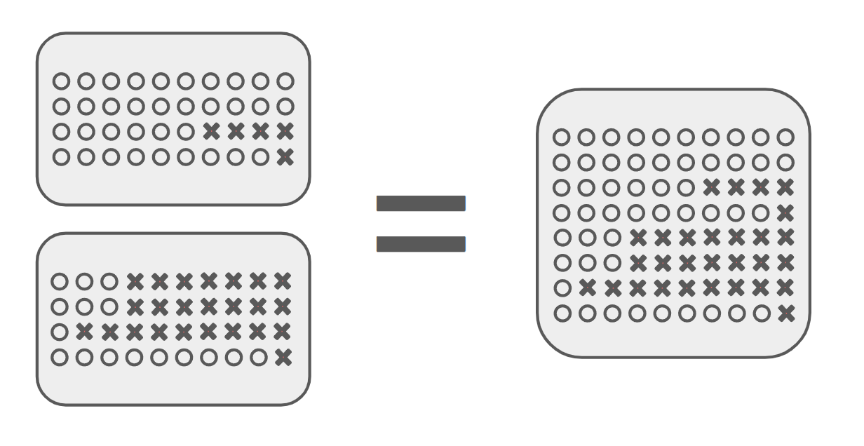
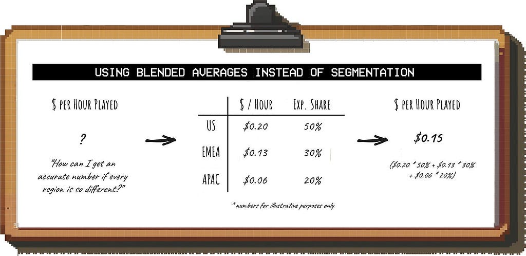
Here’s what you can do in that case to get a quick-and-dirty answer:
Instead of creating multiple separate estimates, you can calculate a blended average for the metric that has the biggest variance across segments.
So if you expect “$ per hour played” to vary substantially across regions, you 1) make an assumption for this metric for each region (e.g. by getting benchmarks, see below) and 2) estimate what the country mix will be:
Image by author
You then use that number for your estimate, eliminating the need to segment.
How detailed should you get?
If you have solid data to base your assumptions on, adding more detail to your analysis can improve the accuracy of your estimate; but only up to a point.
Besides increasing the effort required for the analysis, adding more detail can result in false precision.
Image by author
So what falls into the “too much detail” bucket? For the sake of a quick and dirty estimation, this would include things like:
Segmenting by device type (Smart TV vs. Android vs. iOS)
Considering different engagement levels by day of week
Splitting out CPMs by industry
Modeling the impact of individual games
etc.
Adding this level of detail would increase the number of assumptions exponentially without necessarily making the estimate more accurate.
Step 2: Putting numbers against each metric
Now that you have the inputs to your estimate laid out, it’s time to start putting numbers against them.
Internal data
If you ran an experiment (e.g. you rolled out a prototype for “Netflix games” to some users) and you have results you can use for your estimate, great. But a lot of the time, that’s not the case.
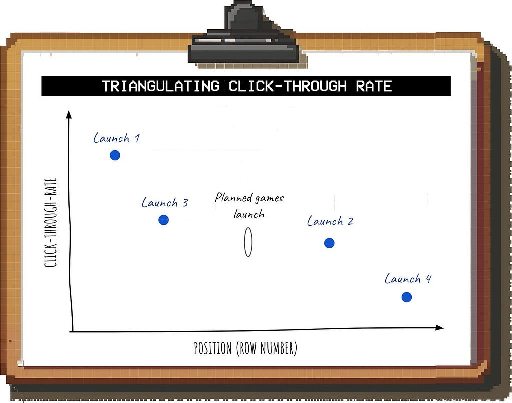
In this case, you have to get creative. For example, let’s say that to estimate our DAU for games, we want to understand how many Netflix users might see and click on the games module in their feed.
To do this, you can compare it against other launches with similar entry points:
What other new additions to the home screen did you launch recently?
How did their performance differ depending on their location (e.g. the first “row” at the top of the screen vs. “below the fold” where you have to scroll to find it)?
Based on the last few launches, you can then triangulate the expected click-through-rate for games:
Image by author
These kind of relationships are often close enough to linear (within a reasonable range) so that this type of approximation yields useful results.
Once you get some actual data from an experiment or the launch, you can refine your assumptions.
External benchmarks
External benchmarks (e.g. industry reports, data vendors) can be helpful to get the right ballpark for a number if internal data is unavailable.
There are a few key considerations:
Pick the closest comparison. For example, casual games on Netflix are closer to mobile games than PC or console games, so pick benchmarks accordingly
Make sure your metric definitions are aligned. Just because a metric in an external report sounds similar doesn’t mean it’s identical to your metric. For example, many companies define “Daily Active Users” differently.
Choose reputable, transparent sources. If you search for benchmarks, you will come across a lot of different sources. Always try to find an original source that uses (and discloses!) a solid methodology (e.g. actual data from a platform rather than surveys). Bonus points if the report is updated regularly so that you can refresh your estimate in the future if necessary.
Deciding on a number
After looking at internal and external data from different sources, you will likely have a range of numbers to choose from for each metric.
Take a look at how wide the range is;this will show you which inputs move the needle on the answer the most.
For example, you might find that the CPM benchmarks from different reports are very similar, but there is a very wide range for how much time users might spend playing your games on a daily basis.
In this case, your focus should be on fine-tuning the “hours played” assumption:
If there is a minimum amount of revenue the business wants to see to invest in games, see if you can reach that level with the most conservative assumption
If there is no minimum threshold, try to use sanity checks to determine a realistic level.
For example, you could compare the play time you’re projecting for games against the total time users currently spend on Netflix.
Even if some of the time is incremental, it’s unrealistic that more than, say, 5% — 10% of the total time is spent on games (most of the users came to Netflix for video content, and there are better gaming offerings out there, after all).
Part 3: How to get people comfortable with your estimates
If you’re doing a quick-and-dirty estimate, people don’t expect it to be perfectly accurate.
However, they still want to understand what it would take for the numbers to be so different that they would lead to a different decision or recommendation.
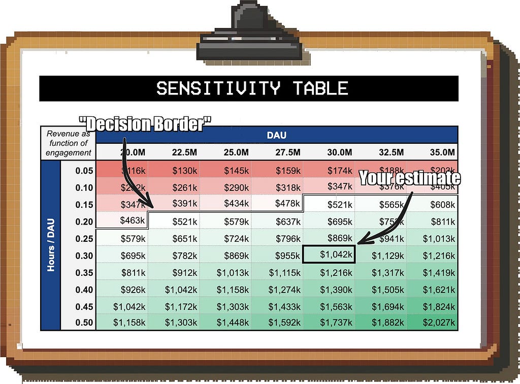
A good way to visualize this is a sensitivity table.
Let’s say the business wants to reach at least $500k in ad revenue per day to even think about launching games. How likely are you to reach this?
On the X and Y axis of the table, you put the two input metrics that you feel least sure about (e.g. “Daily Active Users (DAU)” and “Time Spent per DAU”); the values in the table represent the number you’re estimating (in this case, “Games revenue per day”).
Image by author
You can then compare your best estimate against the minimum requirement of the business; for example, if you’re estimating 30M DAU and 0.3 hours of play time per DAU, you have a comfortable buffer to be wrong on either assumption.
Closing thoughts
While it’s called napkin math, three lines scribbled on a cocktail napkin are rarely enough for a solid estimate.
However, you also don’t need a full-blown 20-tab model to get a directional answer; and often, that directional answer is all you need to move forward.
Once you get comfortable with rough estimates, they allow you move faster than others who are still stuck in analysis paralysis. And with the time you save, you can tackle another project — or go home and do something else.
For more hands-on analytics advice, consider following me here on Medium, on LinkedIn or on Substack.
We use cookies on our website to give you the most relevant experience by remembering your preferences and repeat visits. By clicking “Accept”, you consent to the use of ALL the cookies.
This website uses cookies to improve your experience while you navigate through the website. Out of these, the cookies that are categorized as necessary are stored on your browser as they are essential for the working of basic functionalities of the website. We also use third-party cookies that help us analyze and understand how you use this website. These cookies will be stored in your browser only with your consent. You also have the option to opt-out of these cookies. But opting out of some of these cookies may affect your browsing experience.
Necessary cookies are absolutely essential for the website to function properly. These cookies ensure basic functionalities and security features of the website, anonymously.
Cookie
Duration
Description
cookielawinfo-checkbox-analytics
11 months
This cookie is set by GDPR Cookie Consent plugin. The cookie is used to store the user consent for the cookies in the category "Analytics".
cookielawinfo-checkbox-functional
11 months
The cookie is set by GDPR cookie consent to record the user consent for the cookies in the category "Functional".
cookielawinfo-checkbox-necessary
11 months
This cookie is set by GDPR Cookie Consent plugin. The cookies is used to store the user consent for the cookies in the category "Necessary".
cookielawinfo-checkbox-others
11 months
This cookie is set by GDPR Cookie Consent plugin. The cookie is used to store the user consent for the cookies in the category "Other.
cookielawinfo-checkbox-performance
11 months
This cookie is set by GDPR Cookie Consent plugin. The cookie is used to store the user consent for the cookies in the category "Performance".
viewed_cookie_policy
11 months
The cookie is set by the GDPR Cookie Consent plugin and is used to store whether or not user has consented to the use of cookies. It does not store any personal data.
Functional cookies help to perform certain functionalities like sharing the content of the website on social media platforms, collect feedbacks, and other third-party features.
Performance cookies are used to understand and analyze the key performance indexes of the website which helps in delivering a better user experience for the visitors.
Analytical cookies are used to understand how visitors interact with the website. These cookies help provide information on metrics the number of visitors, bounce rate, traffic source, etc.
Advertisement cookies are used to provide visitors with relevant ads and marketing campaigns. These cookies track visitors across websites and collect information to provide customized ads.