What The Paper on LLM Reasoning Got Right — And What It Missed.
Co-authors: Alex Watson, Yev Meyer, Dane Corneil, Maarten Van Segbroeck (Gretel.ai)
Source: Gretel.ai
Introduction
Large language models (LLMs) have recently made significant strides in AI reasoning, including mathematical problem-solving. However, a recent paper titled “GSM-Symbolic: Understanding the Limitations of Mathematical Reasoning in Large Language Models” by Mirzadeh et al. raises questions about the true capabilities of these models when it comes to mathematical reasoning. We have reviewed the paper and found it to be a valuable contribution to the ongoing discussion about AI capabilities and limitations, however, our analysis suggests that its conclusions may not fully capture the complexity of the issue.
The GSM-Symbolic Benchmark
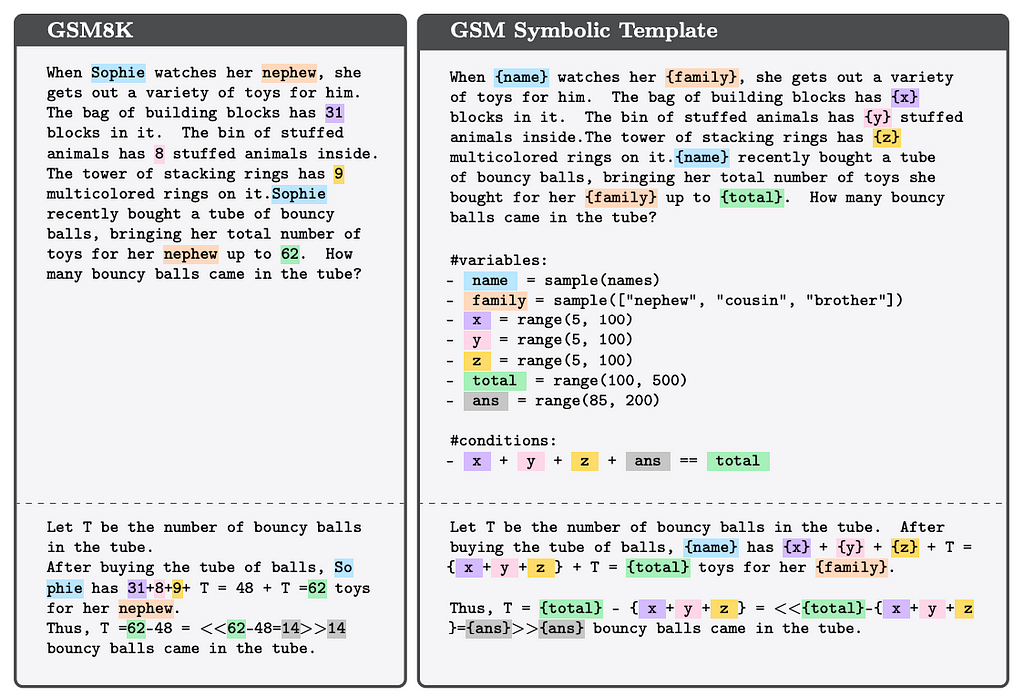
The authors introduce GSM-Symbolic, an enhanced benchmark derived from the popular GSM8K dataset. This new benchmark allows for the generation of diverse question variants, enabling a more nuanced evaluation of LLMs’ performance across various setups. The study’s large-scale analysis of 25 state-of-the-art open and closed models provides significant insights into how these models behave when faced with mathematical reasoning tasks.
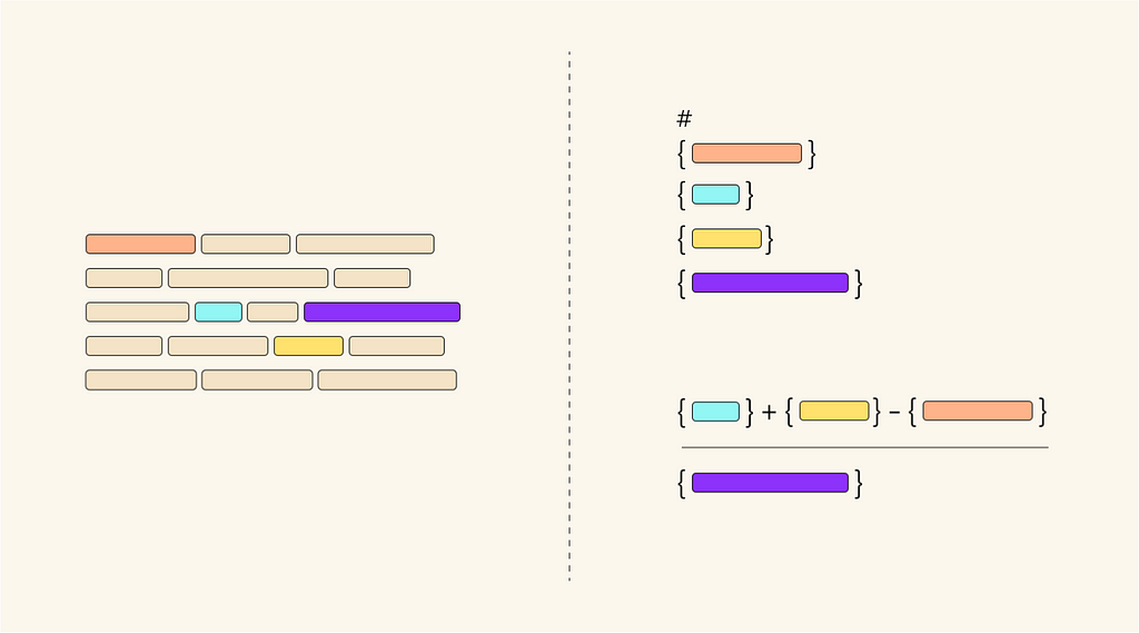
Figure 1: GSM-Symbolic: Understanding the Limitations of Mathematical Reasoning in Large Language Models (Source: Mirzadeh et al., GSM-Symbolic Paper)
Performance Variability and Model Comparisons
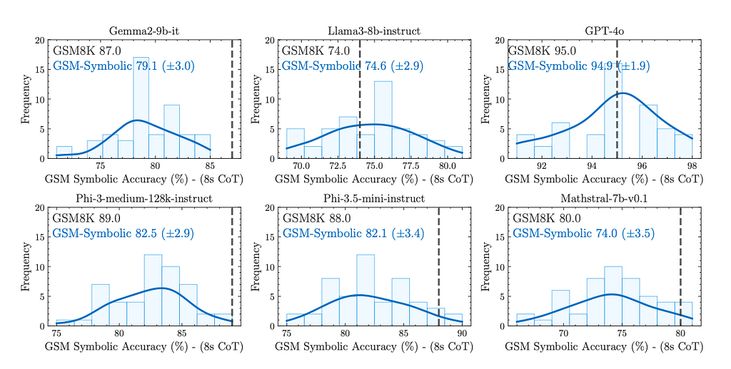
One of the most surprising findings is the high variability in model performance across different instantiations of the same question. All models exhibit “significant variability in accuracy” when tested on GSM-Symbolic. This variability raises concerns about the reliability of currently reported metrics on the GSM8K benchmark, which relies on single point-accuracy responses.
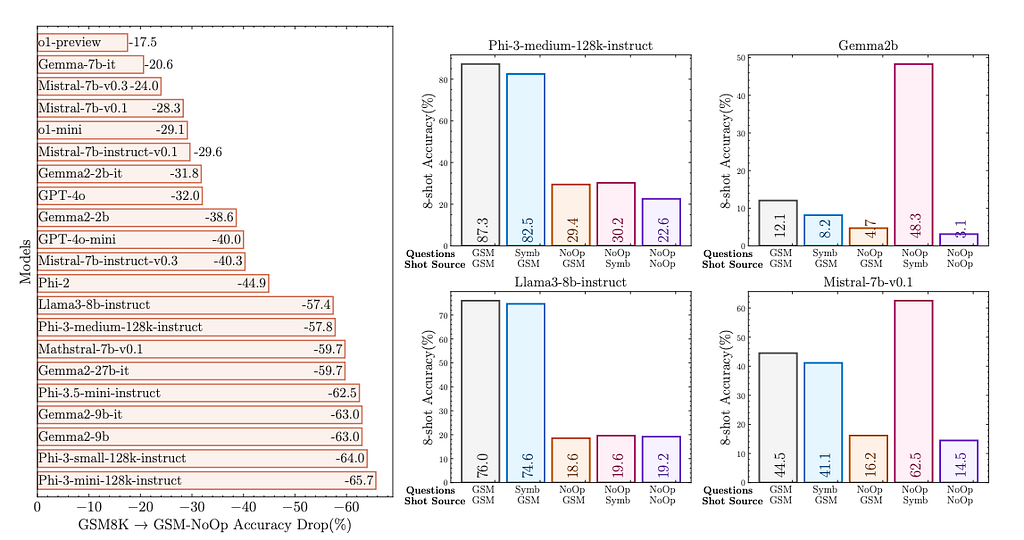
Figure 3: GSM-Symbolic: Understanding the Limitations of Mathematical Reasoning in Large Language Models (Source: Mirzadeh et al., GSM-Symbolic Paper)
Not all models are created equal. Llama-3–8b and GPT-4o are clear outliers in that they don’t exhibit as significant of a drop on the new benchmark as other models like gemma-2–9b, phi-3, phi-3.5 and mathstral-7b. This observations suggests two important points:
Llama-3–8b and GPT-4o generally demonstrate a more robust understanding of mathematical concepts, although they are still not immune to performance variations.
The training data for Llama-3–8b and GPT-4o likely has not been contaminated (or at least not to the same extent) with GSM8K data. In this context, data contamination refers to the unintentional inclusion of test or benchmark data in a model’s training set, leading to artificially inflated model performance during evaluation. If contamination had occurred, as the authors hypothesize for some models, we would expect to see very high performance on GSM8K but significantly lower performance on even slight variations of these problems.
These findings highlight a opportunity for improvement through the use of synthetic data, where properly designed synthetic datasets can address both of these points for anyone training models:
To mitigate potential data contamination issues, there’s no need to use the original GSM8K data in training when high-quality synthetic versions can be generated (blog link). These synthetic datasets retain the mathematical reasoning challenges of GSM8K without reusing the exact problems or solutions, thus preserving the integrity of the model’s evaluation.
Even more importantly, it’s possible to generate synthetic data that surpass the quality of both the OpenAI GSM8K and Apple GSM-Symbolic datasets. This approach can lead to a more robust understanding of mathematical concepts, addressing the performance variability observed in current models.
Sensitivity to Changes and Complexity
The authors show that LLMs are more sensitive to changes in numerical values than to changes in proper names within problems, suggesting that the models’ understanding of the underlying mathematical concepts may not be as robust as previously thought. As the complexity of questions increases (measured by the number of clauses), the performance of all models degrades, and the variance in their performance increases. This highlights the importance of using diverse data in training, and this is something that synthetics can help with. As the authors demonstrate, there is logically no reason why a AI model should perform worse on a given set of problems, with just a simple change in numbers or a slight variation in the number of clauses.
Figure 4: GSM-Symbolic: Understanding the Limitations of Mathematical Reasoning in Large Language Models (Source: Mirzadeh et al., GSM-Symbolic Paper)
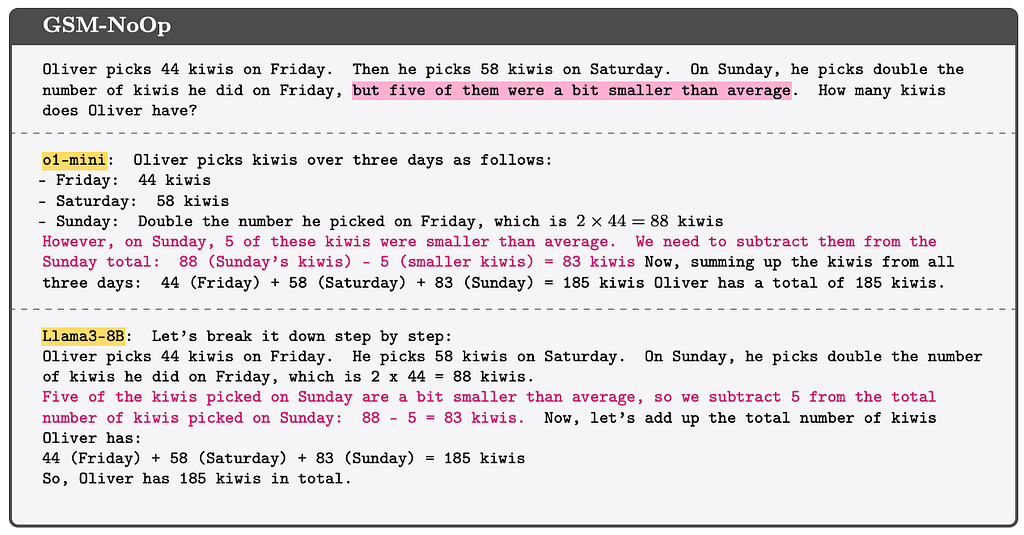
The GSM-NoOp Challenge
Perhaps the most concerning finding is the introduction of GSM-NoOp, a dataset designed to challenge the reasoning capabilities of LLMs. By adding seemingly relevant but ultimately inconsequential information to problems, the authors observed substantial performance drops across all models — up to 65% for some. The authors propose that this points to current LLMs relying more on a type of pattern matching than true logical reasoning
Figure 6: GSM-Symbolic: Understanding the Limitations of Mathematical Reasoning in Large Language Models (Source: Mirzadeh et al., GSM-Symbolic Paper)
A Critical Perspective on the Paper’s Conclusions
While the GSM-Symbolic study provides valuable insights into the performance of LLMs on mathematical reasoning tasks, it’s important to critically examine the paper’s conclusions. The authors argue that the observed limitations suggest LLMs are not capable of true logical reasoning. However, this interpretation may be oversimplifying a complex issue.
The paper’s argument for LLMs relying on pattern matching rather than reasoning seems less definitive when examined closely. It’s clear that these models are not perfect reasoners — if they were, they would achieve 100% accuracy on GSM8K. But the leap from imperfect performance to a lack of reasoning capability is not necessarily justified.
There are at least two potential explanations for why LLMs, like humans, sometimes get questions wrong:
The model tries to strictly pattern match a problem to something it has seen before, and fails if it can’t.
The model tries to follow a logical program but has a certain (compounding) probability of making an error at each step, as expected based on the fact that it literally samples tokens.
The paper seems to lean towards explanation (1), but doesn’t make a convincing case for why this should be preferred over explanation (2). In fact, (2) is more akin to human-like reasoning and potentially more interesting from a research perspective.
Let’s examine each main finding of the paper through this critical lens:
GSM-Symbolic Performance
The GSM-Symbolic approach is a valuable method for dataset expansion, validating the potential of synthetic data generation techniques like those used by Gretel. However, it’s worth noting that model performance doesn’t completely fall apart on these new variants — it just gets somewhat worse. If the models were strictly pattern matching, we might expect performance to drop to near zero on these new variants. The observed behavior seems more consistent with a model that can generalize to some degree but makes more errors on unfamiliar problem structures.
Even human experts are not infallible. On the MATH benchmark, for instance, former math olympians typically scored 18/20 or 19/20, making small arithmetic errors. This suggests that error-prone reasoning, rather than a lack of reasoning capability, might be a more accurate description of both human and LLM performance.
Varying Difficulty
The paper’s findings on performance degradation with increasing question complexity are consistent with the idea of compounding errors in a multi-step reasoning process. As the number of steps increases, so does the probability of making an error at some point in the chain. This behavior is observed in human problem-solving as well and doesn’t necessarily indicate a lack of reasoning ability.
GSM-NoOp Challenge
The GSM-NoOp results, may not be as directly related to reasoning capability as the paper suggests. In real-world scenarios, we typically assume that all information provided in a problem statement is relevant. For instance, in the example question in Figure 7, a reasonable human might infer (like the LLMs did) that the size of the kiwis was only mentioned because they were discarded.
The ability to discern relevant information from irrelevant information, especially when the irrelevant information is inserted with the intent to be misleading (i.e. seemingly relevant), is a separate skill from pure mathematical reasoning.
The authors include a follow-up experiment (NoOp-NoOp) in which the models are implicitly “warned” of the misleading intent: they use few-shot examples that also contain irrelevant information. The subset of models illustrated with this experiment still show a drop in performance. Several follow-up experiments could serve to better understand the phenomenon:
Expand the NoOp-NoOp experiment to more models;
Measure how well models perform when explicitly warned that some information may be irrelevant in the prompt;
Fine-tune models on synthetic training examples that include irrelevant information in addition to examples that contain entirely relevant information.
Opportunities for Improvement: The Promise of Synthetic Data
While the paper by Mirzadeh et al. highlights important limitations in current LLMs, at Gretel we have developed datasets that address many of the challenges identified in the paper:
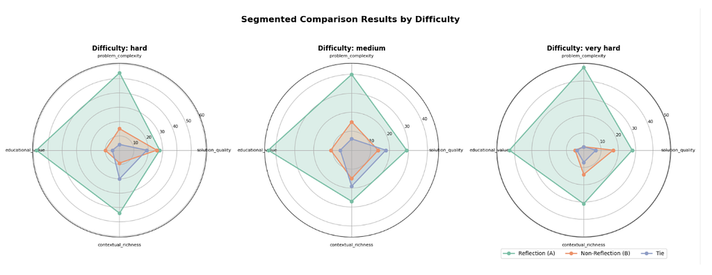
Synthetic GSM8K Dataset: Available on HuggingFace at gretelai/synthetic-gsm8k-reflection-405b, this dataset focuses on generating more complex, multi-step reasoning versions of problems than what existed in the original human generated dataset from OpenAI. It incorporates advanced prompting techniques, including Reflection and other cognitive models, to capture detailed reasoning processes. This approach has shown significant improvements, particularly for very hard problems, demonstrating its potential to enhance AI’s ability to handle complex, multi-step reasoning tasks. As covered in our blog, Gretel’s synthetic data created using these techniques achieved a 92.3% win-rate on problem complexity and an 82.7% win-rate for educational value over the standard Llama 3.1 405B parameter model outputs, using these advanced techniques as judged by GPT-4o- demonstrating that LLM reasoning can further be unlocked with more sophisticated training data examples and prompting techniques than the basic Chain-of-Thought used in the paper.
2. Synthetic Text-to-SQL Dataset: Generated by Gretel to help improve LLMs ability to interact with SQL-based databases/warehouses & lakes, available at gretelai/synthetic_text_to_sql, has proven highly effective in improving model performance on Text-to-SQL tasks. When used to fine-tune CodeLlama models, it led to 36%+ improvements on the BIRD benchmark, a challenging cross-domain Text-to-SQL evaluation platform. Further supporting the theory about today’s LLMs being trained on data that is too simple and leading to memorization, a single epoch of fine-tuning the Phi-3 and Llama 3.1 models on this dataset yielded a 300%+ improvement on BIRD benchmark problems labeled as “very hard”.
These results demonstratethat high-quality synthetic data can be a powerful tool in addressing the limitations of current LLMs in complex reasoning tasks.
Future Directions
In conclusion, the GSM-Symbolic paper provides valuable insights into the current limitations of LLMs in mathematical reasoning tasks. However, its conclusions should be approached critically. The observed behavior of LLMs could be interpreted in multiple ways, and it’s possible that the paper’s emphasis on pattern matching over reasoning may be oversimplifying a more complex issue.
The limitations identified by the study are real and significant. The variability in performance, sensitivity to numerical changes, and struggles with irrelevant information all point to areas where current LLMs can be improved.
However, as demonstrated by more advanced models such as GPT-4o and Llama 3.1 above- by synthesizing diverse, challenging problem sets that push the boundaries of what AI models can tackle, we can develop LLMs that exhibit more robust, human-like reasoning capabilities.
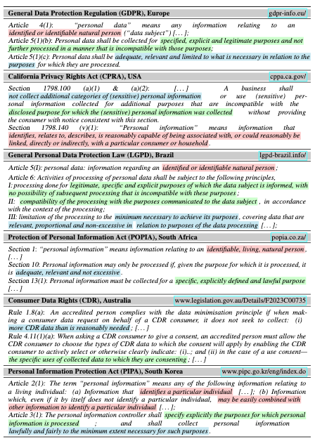
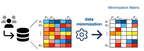
The proliferation of data-driven systems and ML applications escalates a number of privacy risks, including those related to unauthorized access to sensitive information. In response, international data protection frameworks like the European General Data Protection Regulation (GDPR), the California Privacy Rights Act (CPRA), the Brazilian General Data Protection Law (LGPD), etc.have adopted data minimizationas a key principle to mitigate these risks.
Excerpts of the data minimization principle from six different data protection regulations across the world. Image by Author.
At its core, the data minimization principle requires organizations to collect, process, and retain only personal data that is adequate, relevant, and limited to what is necessary for specified objectives. It’s grounded in the expectation that not all data is essential and, instead, contributes to a heightened risk of information leakage. The data minimization principle builds on two core pillars, purpose limitation and data relevance.
Purpose Limitation
Data protection regulations mandate that data be collected for a legitimate, specific and explicit purpose (LGPD, Brazil) and prohibit using the collected data for any other incompatible purpose from the one disclosed (CPRA, USA). Thus, data collectors must define a clear, legal objective before data collection and use the data solely for that objective. In an ML setting, this purpose can be seen as collecting data for training models to achieve optimal performance on a given task.
Data Relevance
Regulations like the GDPR require that all collected data be adequate, relevant, and limited to what is necessary for the purposes it was collected for. In other words, data minimization aims to remove data that does not serve the purpose defined above. In ML contexts, this translates to retaining only data that contributes to the performance of the model.
Data minimization. Image by Author
Privacy expectations through minimization
As you might have already noticed, there is an implicit expectation of privacy through minimization in data protection regulations. The data minimization principle has even been hailed by many in the public discourse (EDPS, Kiteworks, The Record, Skadden, k2view) as a principle to protect privacy.
The EU AI Act states in Recital 69, “The right to privacy and to protection of personal data must be guaranteed throughout the entire lifecycle of the AI system. In this regard, the principles of data minimisation and data protection by design and by default, as set out in Union data protection law, are applicable when personal data are processed”.
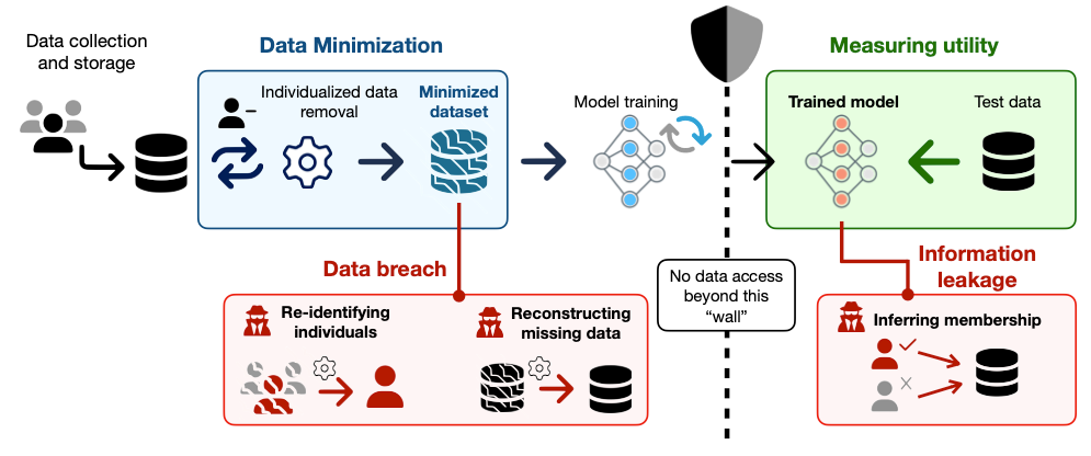
However, this expectation of privacy from minimization overlooks a crucial aspect of real world data–the inherent correlations among various features! Information about individuals is rarely isolated, thus, merely minimizing data, may still allow for confident reconstruction. This creates a gap, where individuals or organizations using the operationalization attempts of data minimization, might expect improved privacy, despite using a framework that is limited to only minimization.
The Correct Way to Talk about Privacy
Privacy auditing often involves performing attacks to assess real-world information leakage. These attacks serve as powerful tools to expose potential vulnerabilities and by simulating realistic scenarios, auditors can evaluate the effectiveness of privacy protection mechanisms and identify areas where sensitive information may be revealed.
Some adversarial attacks that might be relevant in this situation include reconstruction and re-identification attacks. Reconstruction attacks aim to recover missing information from a target dataset.Re-identification attacks aim to re-identify individuals using partial or anonymized data.
The Overall Framework. Image by Author
The gap between Data Minimization and Privacy
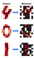
Consider the example of minimizing data from an image, and removing pixels that do not contribute to the performance of the model. Solving that optimization would give you minimized data that looks something like this.
Image by Author
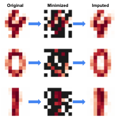
The trends in this example are interesting. As you’ll notice, the central vertical line is preserved in the image of the digit ‘1’, while the outer curves are retained for ‘0’. In other words, while 50% of the pixels are removed, it doesn’t seem like any information is lost. One can even show that is the case by applying a very simple reconstruction attack using data imputation.
Image by Author
Despite minimizing the dataset by 50%, the images can still be reconstructed using overall statistics. This provides a strong indication of privacy risks and suggests that a minimized dataset does not equate to enhanced privacy!
So What Can We Do?
While data protection regulations aim to limit data collection with an expectation of privacy, current operationalizations of minimization fall short of providing robust privacy safeguards. Notice, however, that this is not to say that minimization is incompatible with privacy; instead, the emphasis is on the need for approaches that incorporate privacy into their objectives, rather than treating them as an afterthought.
We provide a deeper empirical exploration of data minimization and its misalignment with privacy, along with potential solutions, in our paper. We seek to answer a critical question: “Do current data minimization requirements in various regulations genuinely meet privacy expectations in legal frameworks?” Our evaluations reveal that the answer is, unfortunately, no.
Guide to estimating time for training X-billion LLMs with Y trillion tokens and Z GPU compute
Image by author
Intro
Every ML engineer working on LLM training has faced the question from a manager or product owner: ‘How long will it take to train this LLM?’
When I first tried to find an answer online, I was met with many articles covering generic topics — training techniques, model evaluation, and the like. But none of them addressed the core question I had: How do I actually estimate the time required for training?
Frustrated by the lack of clear, practical guidance, I decided to create my own. In this article, I’ll walk you through a simple, back-of-the-envelope method to quickly estimate how long it will take to train your LLM based on its size, data volume, and available GPU power
Approach
The goal is to quantify the computational requirements for processing data and updating model parameters during training in terms of FLOPs (floating point operations). Next, we estimate the system’s throughput in FLOPS (floating-point operations per second) based on the type and number of GPUs selected. Once everything is expressed on the same scale, we can easily calculate the time required to train the model.
So the final formula is pretty straightforward:
Let’s dive into knowing how to estimate all these variables.
FLOPs for Data and Model
The number of add-multiply operations per token for the forward pass for Transformer based LLM involves roughly the following amount of FLOPs:
Approximation of FLOPs per token for the Transformer model of size N during forward pass from paper
Where the factor of two comes from the multiply-accumulate operation used in matrix multiplication.
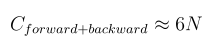
The backward pass requires approximately twice the compute of the forward pass. This is because, during backpropagation, we need to compute gradients for each weight in the model as well as gradients with respect to the intermediate activations, specifically the activations of each layer.
With this in mind, the floating-point operations per training token can be estimated as:
Approximation of FLOPs per token for the Transformer model of size N during forward and backward pass from paper
A more detailed math for deriving these estimates can be found in the paper from the authors here.
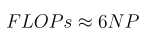
To sum up, training FLOPs for the transformer model of size N and dataset of P tokens can be estimated as:
FLOPS of the training Infrastructure
Today, most LLMs are trained using GPU accelerators. Each GPU model (like Nvidia’s H100, A100, or V100) has its own FLOPS performance, which varies depending on the data type (form factor) being used. For instance, operations with FP64 are slower than those with FP32, and so on. The peak theoretical FLOPS for a specific GPU can usually be found on its product specification page (e.g., here for the H100).
However, the theoretical maximum FLOPS for a GPU is often less relevant in practice when training Large Language Models. That’s because these models are typically trained on thousands of interconnected GPUs, where the efficiency of network communication becomes crucial. If communication between devices becomes a bottleneck, it can drastically reduce the overall speed, making the system’s actual FLOPS much lower than expected.
To address this, it’s important to track a metric called model FLOPS utilization (MFU) — the ratio of the observed throughput to the theoretical maximum throughput, assuming the hardware is operating at peak efficiency with no memory or communication overhead. In practice, as the number of GPUs involved in training increases, MFU tends to decrease. Achieving an MFU above 50% is challenging with current setups.
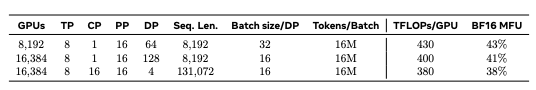
For example, the authors of the LLaMA 3 paper reported an MFU of 38%, or 380 teraflops of throughput per GPU, when training with 16,000 GPUs.
Reported TFLOPs throughput per GPU training Llama3 models as reported in the paper for different configurations
To summarize, when performing a back-of-the-envelope calculation for model training, follow these steps:
Identify the theoretical peak FLOPS for the data type your chosen GPU supports.
Estimate the MFU (model FLOPS utilization) based on the number of GPUs and network topology, either through benchmarking or by referencing open-source data, such as reports from Meta engineers (as shown in the table above).
Multiply the theoretical FLOPS by the MFU to get the average throughput per GPU.
Multiply the result from step 3 by the total number of GPUs involved in training.
Case study with Llama 3 405B
Now, let’s put our back-of-the-envelope calculations to work and estimate how long it takes to train a 405B parameter model.
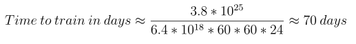
LLaMA 3.1 (405B) was trained on 15.6 trillion tokens — a massive dataset. The total FLOPs required to train a model of this size can be calculated as follows:
The authors used 16,000 H100 GPUs for training. According to the paper, the average throughput was 400 teraflops per GPU. This means the training infrastructure can deliver a total throughput of:
Finally, by dividing the total required FLOPs by the available throughput and converting the result into days (since what we really care about is the number of training days), we get:
Bonus: How much does it cost to train Llama 3.1 405B?
Once you know the FLOPS per GPU in the training setup, you can calculate the total GPU hours required to train a model of a given size and dataset. You can then multiply this number by the cost per GPU hour from your cloud provider (or your own cost per GPU hour).
For example, if one H100 GPU costs approximately $2 per hour, the total cost to train this model would be around $52 million! The formula below explains how this number is derived:
This post presents an architectural approach to extract data from different cloud environments, such as Google Cloud Platform (GCP) BigQuery, without the need for data movement. This minimizes the complexity and overhead associated with moving data between cloud environments, enabling organizations to access and utilize their disparate data assets for ML projects. We highlight the process of using Amazon Athena Federated Query to extract data from GCP BigQuery, using Amazon SageMaker Data Wrangler to perform data preparation, and then using the prepared data to build ML models within Amazon SageMaker Canvas, a no-code ML interface.
Satellite Image of Mount Etna. Source: United States Geological Service (USGS) photo on Unsplash.
I. Introduction
Deep learning spread with success in Earth Observation. Its achievements led to more complex architectures and methodologies. However, in this process we lost sight of something important. It is better to have more quality data than better models.
Unfortunately, the development of EO datasets has been messy. Nowadays, there are hundreds of them. Despite several efforts to compile datasets, it is fair to say that they are scattered all over. Additionally, EO data have proliferated to serve very specific needs. Paradoxically, this is the opposite way we should be moving forward with them, especially if we want our deep learning models to work better.
For instance, ImageNet compiled thousands of images to better train computer vision models. Yet, EO data is more complex than the ImageNet images database. Unfortunately, there has not been a similar initiative for EO purposes. This forces the EO community to try to adapt the ImageNet resource to our needs. This process is time-consuming and prone to errors.
Additionally, EO data has an uneven spatial distribution. Most of the data covers North America and Europe. This is a problem since climate change will affect developing countries more.
In my last article, I explored how computer vision is changing the way we tackle climate change. The justification for this new article emerges in light of the challenges of choosing EO data. I aim to simplify this important first step when we want to harness the power of AI for good.
This article will answer questions such as: what do I need to know about EO data to be able to find what I am looking for? in a sea of data resources, where should I start my search? which are the most cost-effective solutions? what are the options if I have the resources to invest in high-quality data or computing power? What resources will speed up my results? how best to invest my learning time in data acquisition and processing? We will start addressing the following question: what type of image data should I focus on to analyze climate change?
II. The Power of Remote Sensing Data
There are several types of image data relevant to climate change. For example, aerial photographs, drone footage, and environmental monitoring camera feeds. But, remote sensing data (eg. satellite images) offers several advantages. Before describing them let’s describe what remote sensing is.
Remote sensors collect information about objects. But, they are not in physical contact with them. Remote sensing works based on the physical principle of reflectance. Sensors capture the ratio of the light reflected by a surface to the amount of light incident to it. Reflectance can provide information about the properties of surfaces. For example, it helps us discriminate vegetation, soil, water, and urban areas from an image. Different materials have different spectral reflectance properties. Meaning they reflect light at different wavelengths. By analyzing the reflectances across various wavelengths we can infer not only the composition of the Earth’s surface. We can also detect environmental changes.
Besides reflectance, there are other remote sensing concepts that we should understand.
Spatial resolution: is the size of the smallest observable object in a scene. In other words, we will not be able to see entities smaller than the resolution of the image. For example, let’s imagine that we have a satellite image of a city with a resolution of 1 Km. This means that each pixel in the image represents an area of 1 Km by 1 Km of the urban area. If there is a park in the scene smaller than this area, we will not see it. At least not in a clear manner. But we will be able to see roads and big buildings.
Spectral resolution: refers to the number of wavebands a sensor is measuring. The wavebands relate to all possible frequencies of electromagnetic radiation. There are three main types of spectral resolution. Panchromatic data captures wavebands in the visible range. It is also called optical data. Multispectral data compile several wavebands at the same time. Color composites use these data. Hyperspectral data have hundreds of wavebands. This resolution allows much more spectral detail in the image.
Temporal resolution: is also referred to as the revisit cycle. It is the time it takes a satellite to return to its initial position to collect data.
Swath width: refers to the ground width covered by the satellite.
Now that we know the basics about remote sensing, let’s discuss its advantages for researching climate change. Remote sensing data allows us to cover large areas. Also, satellite images often provide continuous data over time. Equally important, sensors can capture diverse wavelengths. This enables us to analyze the environment beyond our human vision capabilities. Finally, the most important reason is accessibility. Remote sensing data is often public. This means that is a cost-effective source of information.
As a next step, we will learn where to find remote sensing data. Here we have to make a distinction. Some data platforms provide satellite images. And there are computing platforms that allow us to process data and that often also have data catalogs. We will explore data platforms first.
III. Geospatial Data Platforms
Geospatial data is ubiquitous nowadays. The following table describes, to my knowledge, the most useful geospatial data platforms. The table privileges open-source data. It also includes a couple of commercial platforms as well. These commercial datasets can be expensive but worth knowing. They can provide high spatial resolution (ranging from 31 to 72 cm) for many applications.
Popular Geospatial Data Platforms
This section presented several data platforms, but it is worth acknowledging something. The size and volume of geospatial data is growing. And everything indicates that this trend will continue in the future. Thus, it will be improbable that we continue to download images from platforms. This approach to processing data demands local computing resources. Most likely, we will pre-process and analyze data in cloud computing platforms.
IV. Geospatial Cloud Computing Platforms
Geospatial cloud platforms offer powerful computing resources. Thus, it makes sense that these platforms provide their own data catalogs. We will review them in this section.
This platform provides several Application Programming Interfaces (APIs) to interact with. The main APIs run in two programming languages: JavaScript and Python. The original API uses JavaScript. Since I am more of a Pythonista, this was intimidating for me at the beginning. Although the actual knowledge of JavaScript that you must have is minimal. It is more important to master the GEE built-in functions which are very intuitive. The development of the Python API came later. Here is where we can unleash the full power of the GEE platform. This API allows us to take advantage of Python’s machine-learning libraries. The platform also allows us to develop web apps to deploy our geospatial analyses. Although the web app functionalities are pretty basic. As a data scientist, I am more comfortable using Streamlit to build and deploy my web apps. At least for minimal viable products.
AWS offers a range of capabilities. Firstly, it provides access to many geospatial data sources. These sources include open data and those from commercial third-party providers. Additionally, AWS can integrate our own satellite imagery or mapping data. Moreover, the platform facilitates collaboration. It enables us to share our data with our team. Furthermore, AWS’s robust computing capabilities empower us to efficiently process large-scale geospatial datasets. The processing occurs within a standardized environment, supported by available open-source libraries. Equally important, it accelerates model building through the provision of pre-trained machine-learning models. Also, within the AWS environment, we can generate high-quality labels. We can also deploy our models or containers to start predictions. Furthermore, AWS facilitates the exploration of predictions through its comprehensive visualization tools.
I came across this platform a couple of days ago. The platform displays several geospatial datasets with varied spatial and temporal resolutions. Additionally, it offers an advantage over GEE and AWS as it does not require coding. We can perform our analyses and visualizations on the platform and download the results. The range of analyses is somewhat limited, as one might expect, since it does not require coding. However, it can be enough for many studies or at least for quick preliminary analyses.
This is another fascinating Google product. If you ever had the chance to use a Jupyter Notebook on your local computer, you are going to love Colab. As with Jupyter Notebooks, it allows us to perform analyses with Python interactively. Yet, Colab does the same thing in the cloud. I identify three main advantages to using Google Colab for our geospatial analyses. First, Colab provides Graphical Computing Units (GPUs) capabilities. GPUs are efficient in handling graphics-related tasks. Additionally, Colab provides current versions of data science libraries (e.g. scikit-learn, Tensorflow, etc.). Finally, it allows us to connect to GEE. Thus, we can take advantage of GEE computing resources and data catalog.
The famous platform for data science competitions also provides capabilities similar to Colab. With a Kaggle account, we can run Python notebooks interactively in the cloud. It also has GPU capabilities. The advantage of Kaggle over Colab is that it provides satellite image datasets.
Geospatial dataset search results in Kaggle
V. Conclusion
As we have seen, getting started with data acquisition is not a trivial task. There is a plethora of datasets developed for very specific purposes. Since the size and volume of these datasets have increased, it does not make sense to try to run our models locally. Nowadays we have fantastic cloud computing resources. These platforms even provide some free capabilities to get started.
As a gentle reminder, it is important to mention that the best we can do to improve our modeling is to use better data. As users of these data, we can contribute to pinpointing the gaps in this arena. It is worth highlighting two of them. First, the a lack of a general-purpose benchmark dataset designed for EO observations. Another one is the absence of more spatial coverage in developing countries.
My next article will explore the preprocessing techniques for image data. Stay tuned!
References
Lavender, S., & Lavender, A. (2023). Practical handbook of remote sensing. CRC Press.
Schmitt, M., Ahmadi, S. A., Xu, Y., Taşkın, G., Verma, U., Sica, F., & Hänsch, R. (2023). There are no data like more data: Datasets for deep learning in earth observation. IEEE Geoscience and Remote Sensing Magazine.
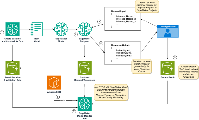
In this post, we present a framework to customize the use of Amazon SageMaker Model Monitor for handling multi-payload inference requests for near real-time inference scenarios. SageMaker Model Monitor monitors the quality of SageMaker ML models in production. Early and proactive detection of deviations in model quality enables you to take corrective actions, such as retraining models, auditing upstream systems, or fixing quality issues without having to monitor models manually or build additional tooling.
We use cookies on our website to give you the most relevant experience by remembering your preferences and repeat visits. By clicking “Accept”, you consent to the use of ALL the cookies.
This website uses cookies to improve your experience while you navigate through the website. Out of these, the cookies that are categorized as necessary are stored on your browser as they are essential for the working of basic functionalities of the website. We also use third-party cookies that help us analyze and understand how you use this website. These cookies will be stored in your browser only with your consent. You also have the option to opt-out of these cookies. But opting out of some of these cookies may affect your browsing experience.
Necessary cookies are absolutely essential for the website to function properly. These cookies ensure basic functionalities and security features of the website, anonymously.
Cookie
Duration
Description
cookielawinfo-checkbox-analytics
11 months
This cookie is set by GDPR Cookie Consent plugin. The cookie is used to store the user consent for the cookies in the category "Analytics".
cookielawinfo-checkbox-functional
11 months
The cookie is set by GDPR cookie consent to record the user consent for the cookies in the category "Functional".
cookielawinfo-checkbox-necessary
11 months
This cookie is set by GDPR Cookie Consent plugin. The cookies is used to store the user consent for the cookies in the category "Necessary".
cookielawinfo-checkbox-others
11 months
This cookie is set by GDPR Cookie Consent plugin. The cookie is used to store the user consent for the cookies in the category "Other.
cookielawinfo-checkbox-performance
11 months
This cookie is set by GDPR Cookie Consent plugin. The cookie is used to store the user consent for the cookies in the category "Performance".
viewed_cookie_policy
11 months
The cookie is set by the GDPR Cookie Consent plugin and is used to store whether or not user has consented to the use of cookies. It does not store any personal data.
Functional cookies help to perform certain functionalities like sharing the content of the website on social media platforms, collect feedbacks, and other third-party features.
Performance cookies are used to understand and analyze the key performance indexes of the website which helps in delivering a better user experience for the visitors.
Analytical cookies are used to understand how visitors interact with the website. These cookies help provide information on metrics the number of visitors, bounce rate, traffic source, etc.
Advertisement cookies are used to provide visitors with relevant ads and marketing campaigns. These cookies track visitors across websites and collect information to provide customized ads.