This post introduces an innovative voice-based application workflow that harnesses the power of Amazon Bedrock, Amazon Transcribe, and React to systematically capture and document institutional knowledge through voice recordings from experienced staff members. Our solution uses Amazon Transcribe for real-time speech-to-text conversion, enabling accurate and immediate documentation of spoken knowledge. We then use generative AI, powered by Amazon Bedrock, to analyze and summarize the transcribed content, extracting key insights and generating comprehensive documentation.
Global Resiliency is a new Amazon Lex capability that enables near real-time replication of your Amazon Lex V2 bots in a second AWS Region. When you activate this feature, all resources, versions, and aliases associated after activation will be synchronized across the chosen Regions. With Global Resiliency, the replicated bot resources and aliases in the […]
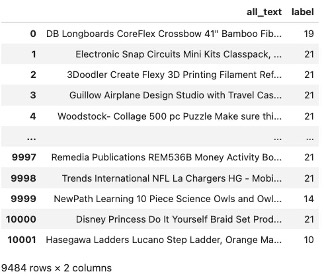
In this post, we showcase how to fine-tune a sentence transformer specifically for classifying an Amazon product into its product category (such as toys or sporting goods). We showcase two different sentence transformers, paraphrase-MiniLM-L6-v2 and a proprietary Amazon large language model (LLM) called M5_ASIN_SMALL_V2.0, and compare their results.
Exploring the future of multimodal AI Agents and the Impact of Screen Interaction
Image created by author using GPT4o
Introduction: The ever-evolving AI Agent Landscape
Recent announcements from Anthropic, Microsoft, and Apple are changing the way we think about AI Agents. Today, the term “AI Agent” is oversaturated — nearly every AI-related announcement refers to agents, but their sophistication and utility vary greatly.
At one end of the spectrum, we have advanced agents that leverage multiple loops for planning, tool execution, and goal evaluation, iterating until they complete a task. These agents might even create and use memories, learning from their past mistakes to drive future successes. Determining what makes an effective agent is a very active area of AI research. It involves understanding what attributes make a successful agent (e.g., how should the agent plan, how should it use memory, how many tools should it use, how should it keep track of it’s task) and the best approach to configure a team of agents.
On the other end of the spectrum, we find AI agents that execute single purpose tasks that require little if any reasoning. These agents are often more workflow focused. For example, an agent that consistently summarizes a document and stores the result. These agents are typically easier to implement because the use cases are narrowly defined, requiring less planning or coordination across multiple tools and fewer complex decisions.
With the latest announcements from Anthropic, Microsoft, and Apple, we’re witnessing a shift from text-based AI agents to multimodal agents. This opens up the potential to give an agent written or verbal instructions and allow it to seamlessly navigate your phone or computer to complete tasks. This has great potential to improve accessibility across devices, but also comes with significant risks. Anthropic’s computer use announcement highlights the risks of giving AI unfettered access to your screen, and provides risk mitigation tactics like running Claude in a dedicated virtual machine or container, limiting internet access to an allowlist of permitted domains, including human in the loop checks, and avoiding giving the model access to sensitive data. They note that no content submitted to the API will be used for training.
Key Announcements from Anthropic, Microsoft, and Apple:
Anthropic’s Claude 3.5 Sonnet: Giving AI the Power to Use Computers
Overview: The goal of Computer Use is to give AI the ability to interact with a computer the same way a human would. Ideally Claude would be able to open and edit documents, click to various areas of the page, scroll and read pages, run and execute command line code, and more. Today, Claude can follow instructions from a human to move a cursor around the computer screen, click on relevant areas of the screen, and type into a virtual keyboard. Claude Scored 14.9% on the OSWorld benchmark, which is higher than other AI models on the same benchmark, but still significantly behind humans (humans typically score 70–75%).
How it works: Claude looks at user submitted screenshots and counts pixels to determine where it needs to move the cursor to complete the task. Researchers note that Claude was not given internet access during training for safety reasons, but that Claude was able to generalize from training tasks like using a calculator and text-editor to more complex tasks. It even retried tasks when it failed. Computer use includes three Anthropic defined tools: computer, text editor, and bash. The computer tool is used for screen navigation, text editor is used for viewing, creating, and editing text files, and bash is used to run bash shell commands.
Challenges: Despite it’s promising performance, there’s still a long way to go for Claude’s computer use abilities. Today it struggles with scrolling, overall reliability, and is vulnerable to prompt injections.
How to Use: Public beta available through the Anthropic API. Computer use can be combined with regular tool use.
Microsoft’s OmniParser & GPT-4V: Making Screens Understandable and Actionable for AI
Overview: OmniParser is designed to parse screenshots of user interfaces and transform them into structured outputs. These outputs can be passed to a model like GPT-4V to generate actions based on the detected screen elements. OmniParser + GPT-4V were scored on a variety of benchmarks including Windows Agent Arena which adapts the OSWorld benchmark to create Windows specific tasks. These tasks are designed to evaluate an agents ability to plan, understand the screen, and use tools, OmniParser & GPT-4V scored ~20%.
How it Works: OmniParser combines multiple fine-tuned models to understand screens. It uses a finetuned interactable icon/region detection model (YOLOv8), a finetuned icon description model (BLIP-2 or Florence2), and an OCR module. These models are used to detect icons and text and generate descriptions before sending this output to GPT-4V which decides how to use the output to interact with the screen.
Challenges: Today, when OmniParser detects repeated icons or text and passes them to GPT-4V, GPT-4V usually fails to click on the correct icon. Additionally, OmniParser is subject to OCR output so if the bounding box is off, the whole system might fail to click on the appropriate area for clickable links. There are also challenges with understanding certain icons since sometimes the same icon is used to describe different concepts (e.g., three dots for loading versus for a menu item).
How to Use: OmniParser is available on GitHub & HuggingFace you will need to install the requirements and load the model from HuggingFace, next you can try running the demo notebooks to see how OmniParser breaks down images.
Apple’s Ferret-UI: Bringing Multimodal Intelligence to Mobile UIs
Overview: Apple’s Ferret (Refer and Ground Anything Anywhere at Any Granularity) has been around since 2023, but recently Apple released Ferret-UI a MLLM (Multimodal Large Language Model) which can execute “referring, grounding, and reasoning tasks” on mobile UI screens. Referring tasks include actions like widget classification and icon recognition. Grounding tasks include tasks like find icon or find text. Ferret-UI can understand UIs and follow instructions to interact with the UI.
How it Works: Ferret-UI is based on Ferret and adapted to work on finer grained images by training with “any resolution” so it can better understand mobile UIs. Each image is split into two sub-images which have their own features generated. The LLM uses the full image, both sub-images, regional features, and text embeddings to generate a response.
Challenges: Some of the results cited in the Ferret-UI paper demonstrate instances where Ferret predicts nearby text instead of the target text, predicts valid words when presented with a screen that has misspelled words, it also sometimes misclassifies UI attributes.
How to Use: Apple made the data and code available on GitHub for research use only. Apple released two Ferret-UI checkpoints, one built on Gemma-2b and one built on Llama-3–8B. The Ferret-UI models are subject to the licenses for Gemma and Llama while the dataset allows non-commercial use.
Summary: Three Approaches to AI Driven Screen Navigation
In summary, each of these systems demonstrate a different approach to building multimodal agents that can interact with computers or mobile devices on our behalf.
Anthropic’s Claude 3.5 Sonnet focuses on general computer interaction where Claude counts pixels to appropriately navigate the screen. Microsoft’s OmniParser addresses specific challenges for breaking down user interfaces into structured outputs which are then sent to models like GPT-4V to determine actions. Apple’s Ferret-UI is tailored to mobile UI comprehension allowing it to identify icons, text, and widgets while also executing open-ended instructions related to the UI.
Across each system, the workflow typically follows two key phases one for parsing the visual information and one for reasoning about how to interact with it. Parsing screens accurately is critical for properly planning how to interact with the screen and making sure the system reliably executes tasks.
Conclusion: Building Smarter, Safer AI Agents
In my opinion, the most exciting aspect of these developments is how multimodal capabilities and reasoning frameworks are starting to converge. While these tools offer promising capabilities, they still lag significantly behind human performance. There are also significant AI safety concerns which need to be addressed when implementing any agentic system with screen access.
One of the biggest benefits of agentic systems is their potential to overcome the cognitive limitations of individual models by breaking down tasks into specialized components. These systems can be built in many ways. In some cases, what appears to the user as a single agent may, behind the scenes, consist of a team of sub-agents — each managing distinct responsibilities like planning, screen interaction, or memory management. For example, a reasoning agent might coordinate with another agent that specializes in parsing screen data, while a separate agent curates memories to enhance future performance.
Alternatively, these capabilities might be combined within one robust agent. In this setup, the agent could have multiple internal planning modules— one focused on planning the screen interactions and another focused on managing the overall task. The best approach to structuring agents remains to be seen, but the goal remains the same: to create agents that perform reliably overtime, across multiple modalities, and adapt seamlessly to the user’s needs.
Distance map from Mississippi State University (by author)
Have you noticed some of the “distance from” maps on social media? I just saw one by Todd Jones that shows how far you are from a national park at any location in the Lower 48 States.
These proximity maps are fun and useful. If you’re a survivalist, you might want to relocate as far as possible from a potential nuclear missile target; if you’re an avid fisherman, you might want to stick close to a Bass Pro Shop.
I went to graduate school with a British guy who knew almost nothing about American college football. Despite this, he did very well in our weekly betting pool. One of his secrets was to bet against any team that had to travel more than 300 miles to play, assuming the competing teams were on par, or the home team was favored.
In this Quick Success Data Science project, we’ll use Python to make “distance from” maps for college football teams in the Southeastern Conference (SEC). We’ll find which team has to make the longest trips, on average, to play other teams, and which has the shortest trips. We’ll then contour up these distances on a map of the southeastern US. In addition, we’ll look at how to grid and contour other continuous data, like temperatures.
The Code
Here’s the full code (written in JupyterLab). I’ll break down the code blocks in the following sections.
import numpy as np
import matplotlib.pyplot as plt
import pandas as pd
import geopandas as gpd
from geopy.distance import great_circle
# Calculate distances from SCHOOL to every point in grid: distances = np.zeros(xx.shape) for i in range(xx.shape[0]): for j in range(xx.shape[1]): point_coords = (yy[i, j], xx[i, j]) distances[i, j] = great_circle(school_coords, point_coords).miles
# Load state boundaries from US Census Bureau: url = 'https://www2.census.gov/geo/tiger/GENZ2021/shp/cb_2021_us_state_20m.zip' states = gpd.read_file(url)
# Filter states within the map limits: states = states.cx[x_min:x_max, y_min:y_max]
# Plot the state boundaries: states.boundary.plot(ax=ax, linewidth=1, edgecolor='black')
# Add labels for the schools: for i, school in enumerate(df['school']): ax.annotate( school, (df['longitude'][i], df['latitude'][i]), textcoords="offset points", xytext=(2, 1), ha='left', fontsize=8 )
ax.set_xlabel('Longitude') ax.set_ylabel('Latitude') ax.set_title(f'Distance from {SCHOOL} to Other SEC Schools')
import numpy as np import matplotlib.pyplot as plt import pandas as pd import geopandas as gpd from geopy.distance import great_circle
Loading Data
For the input data, I made a list of the schools and then had ChatGPT produce the dictionary with the lat-lon coordinates. The dictionary was then converted into a pandas DataFrame named df.
The code will produce a distance map from one of the listed SEC schools. We’ll assign the school’s name (typed exactly as it appears in the dictionary) to a constant named SCHOOL.
# Pick a school to plot the distance from.
# Use the same name as in the data dict:
SCHOOL = 'Texas'
To control the “smoothness” of the contours, we’ll use a constant named RESOLUTION. The larger the number, the finer the underlying grid and thus the smoother the contours. Values around 500–1,000 produce good results.
# Set the grid resolution.
# Larger = higher res and smoother contours:
RESOLUTION = 500
Getting the School Location
Now to get the specified school’s map coordinates. In this case, the school will be the University of Texas in Austin, Texas.
# Get coordinates for SCHOOL:
school_index = df[df['school'] == SCHOOL].index[0]
school_coords = df.loc[school_index, ['latitude', 'longitude']].to_numpy()
The first line identifies the DataFrame index of the school specified by the SCHOOL constant. This index is then used to get the school’s coordinates. Because index returns a list of indices where the condition is true, we use [0] to get the first (presumably only) item in this list.
Next, we extract latitude and longitude values from the DataFrame and convert them into a NumPy array with the to_numpy() method.
If you’re unfamiliar with NumPy arrays, check out this article:
Before we make a contour map, we must build a regular grid and populate the grid nodes (intersections) with distance values. The following code creates the grid.
The first step here is to get the min and max values (x_min, x_max and y_min, y_max) of the longitude and latitude from the DataFrame.
Next, we use NumPy’s meshgrid() method to create a grid of points within the bounds defined by the min and max latitudes and longitudes.
Here’s how the grid looks for a resolution of 100:
The grid nodes of a grid created with resolution = 100 (by author)
Each node will hold a value that can be contoured.
Calculating Distances
The following code calculates concentric distances from the specified school.
# Calculate distances from SCHOOL to every point in grid:
distances = np.zeros(xx.shape)
for i in range(xx.shape[0]):
    for j in range(xx.shape[1]):
        point_coords = (yy[i, j], xx[i, j])
        distances[i, j] = great_circle(school_coords, point_coords).miles
The first order of business is to initialize a NumPy array called distances. It has the same shape as thexx grid and is filled with zeroes. We’ll use it to store the calculated distances from SCHOOL.
Next, we loop over the rows of the grid, then, in a nested loop, iterate over the columns of the grid. With each iteration we retrieve the coordinates of the point at position (i, j) in the grid, with yy and xx holding the grid coordinates.
The final line calculates the great-circle distance (the distance between two points on a sphere) from the school to the current point coordinates (point_coords). The ultimate result is an array of distances with units in miles.
Creating the Map
Now that we have x, y, and distance data, we can contour the distance values and make a display.
We start by setting up a Matplotlib figure of size 10 x 8. If you’re not familiar with the fig, ax terminology, check out this terrific article for a quick introduction:
To draw the color-filled contours we use Matplotlib’s contourf() method. It uses the xx, yy, and distancesvalues, the coolwarm colormap, and a slight amount of transparency (alpha=0.9).
The default color bar for the display is lacking, in my opinion, so we customize it somewhat. The fig.colorbar() method adds a color bar to the plot to indicate the distance scale. The shrink argument keeps the height of the color bar from being disproportionate to the plot.
Finally, we use Matplotlib’s scatter() method to add the school locations to the map, with a marker size of 2. Later, we’ll label these points with the school names.
Adding the State Boundaries
The map currently has only the school locations to use as landmarks. To make the map more relatable, the following code adds state boundaries.
# Load state boundaries from US Census Bureau:
url = 'https://www2.census.gov/geo/tiger/GENZ2021/shp/cb_2021_us_state_20m.zip'
states = gpd.read_file(url)

# Filter states within the map limits:
states = states.cx[x_min:x_max, y_min:y_max]

# Plot the state boundaries:
states.boundary.plot(ax=ax, linewidth=1, edgecolor='black')
The third line uses geopandas’ cx indexer method for spatial slicing. It filters geometries in a GeoDataFrame based on a bounding box defined by the minimum and maximum x (longitude) and y (latitude) coordinates. Here, we filter out all the states outside the bounding box.
Adding Labels and a Title
The following code finishes the plot by tying up a few loose ends, such as adding the school names to their map markers, labeling the x and y axes, and setting an updateable title.
# Add labels for the schools:
for i, school in enumerate(df['school']):
    ax.annotate(
        school,
        (df['longitude'][i], df['latitude'][i]),
        textcoords="offset points",
        xytext=(2, 1),
        ha='left',
        fontsize=8
    )

ax.set_xlabel('Longitude')
ax.set_ylabel('Latitude')
ax.set_title(f'Distance from {SCHOOL} to Other SEC Schools')
fig.savefig('distance_map.png', dpi=600)
plt.show()
To label the schools, we use a for loop and enumeration to choose the correct coordinates and names for each school and use Matplotlib’s annotate() method to post them on the map. We use annotate() rather than the text() method to access the xytext argument, which lets us shift the label to where we want it.
Finding the Shortest and Longest Average Distances
Instead of a map, what if we want to find the average travel distance for a school? Or find which schools have the shortest and longest averages? The following code will do these using the previous df DataFrame and techniques like the great_circle() method that we used before:
# Calculate average distances between each school and the others coords = df[['latitude', 'longitude']].to_numpy() distance_matrix = np.zeros((len(coords), len(coords)))
for i in range(len(coords)): for j in range(len(coords)): distance_matrix[i, j] = great_circle((coords[i][0], coords[i][1]), (coords[j][0], coords[j][1])).miles
print(f"School with shortest average distance: {shortest_avg_distance_school}") print(f"School with longest average distance: {longest_avg_distance_school}")
School with shortest average distance: Miss State
School with longest average distance: Texas
Mississippi State University, near the center of the SEC, has the shortest average travel distance (320 miles). The University of Texas, on the far western edge of the conference, has the longest (613 miles).
NOTE: These average distances do not take into account annual schedules. There aren’t enough games in a season for all the teams to play each other, so the averages in a given year may be shorter or longer than the ones calculated here. Over three-year periods, however, each school will rotate through all the conference teams.
Finding the Minimum Distance to an SEC School
Remember at the start of this article I mentioned a distance-to-the-nearest-national-park map? Now I’ll show you how to make one of these, only we’ll use SEC schools in place of parks.
All you have to do is take our previous code and replace the “calculate distances” block with this snippet (plus adjust the plot’s title text):
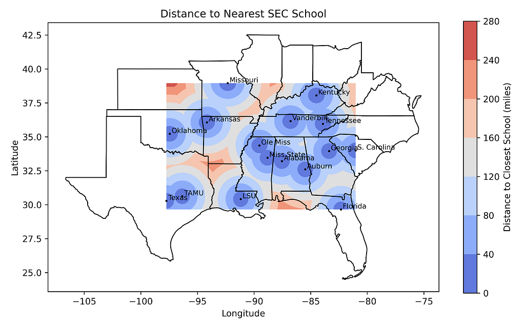
# Calculate minimum distance to any school from every point in the grid:
distances = np.zeros(xx.shape)
for i in range(xx.shape[0]):
    for j in range(xx.shape[1]):
        point_coords = (yy[i, j], xx[i, j])
        distances[i, j] = min(great_circle(point_coords,
                                           (df.loc[k, 'latitude'],
                                            df.loc[k, 'longitude'])).miles
                                   for k in range(len(df)))
Distance to nearest SEC school within the bounding box (by author)
This may take a few minutes, so be patient (or drop the resolution on the grid before running).
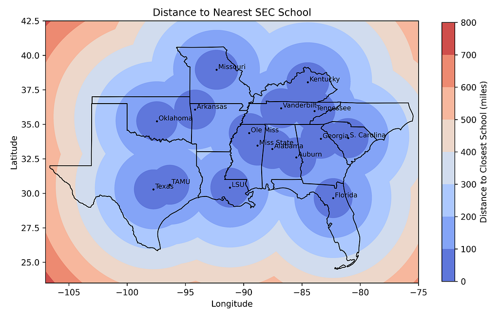
For a more ascetic map, expand the size of the grid by making this edit:
And adjust the lat-lon dimensions for the state boundaries with this substitution:
# Filter states within the map limits
states = states.cx[-100:-80, 25:36.5]
Here’s the result:
Distance to nearest school map with new limits and states (by author)
There are more fancy things we can do, such as manually removing states not in the SEC and clipping the contoured map to the outer state boundaries. But I’m tired now, so those are tasks for another article!
Gridding and Contouring Other Continuous Data
In the previous examples, we started with location data and calculated “distance from” directly from the map coordinates. In many cases, you’ll have additional data, such as temperature measurements, that you’ll want to contour.
Here’s an example script for doing this, built off what we did before. I’ve replaced the school names with temperatures in degrees Fahrenheit. I’ve also used SciPy to grid the data, as a change of pace.
import numpy as np import matplotlib.pyplot as plt import pandas as pd import geopandas as gpd from scipy.interpolate import griddata
# Load state boundaries from US Census Bureau url = 'https://www2.census.gov/geo/tiger/GENZ2021/shp/cb_2021_us_state_20m.zip' states = gpd.read_file(url)
# Filter states within the map limits states = states.cx[x_min:x_max, y_min:y_max]
# Plot the state boundaries states.boundary.plot(ax=ax, linewidth=1, edgecolor='black')
# Add data points and labels scatter = ax.scatter(df.longitude, df.latitude, c='black', edgecolors='white', s=10)
for i, row in df.iterrows(): ax.text(row['longitude'], row['latitude'], f"{round(row['temp'])}°F", fontsize=8, ha='right', color='k')
# Set labels and title ax.set_xlabel('Longitude') ax.set_ylabel('Latitude') ax.set_title('Temperature Contours') plt.savefig('temperature_map.png', dpi=600) plt.show()
Here’s the resulting temperature map:
The temperature contour map (by author)
This technique works well for any continuously and smoothly varying data, such as temperature, precipitation, population, etc.
Summary
Contouring data on maps is common practice for many professions, including geology, meteorology, economics, and sociology. In this article, we used a slew of Python libraries to make maps of the distance from specific colleges, and then from multiple colleges. We also looked at ways to grid and contour other continuous data, such as temperature data.
Thanks!
Thanks for reading and please follow me for more Quick Success Data Science projects in the future.
Data science practitioners encounter numerous challenges when handling diverse data types across various projects, each demanding unique processing methods. A common obstacle is working with data formats that traditional machine learning models struggle to process effectively, resulting in subpar model performance. Since most machine learning algorithms are optimized for numerical data, transforming categorical data into numerical form is essential. However, this often oversimplifies complex categorical relationships, especially when the feature have high cardinality — meaning a large number of unique values — which complicates processing and impedes model accuracy.
High cardinality refers to the number of unique elements within a feature, specifically addressing the distinct count of categorical labels in a machine learning context. When a feature has many unique categorical labels, it has high cardinality, which can complicate model processing. To make categorical data usable in machine learning, these labels are often converted to numerical form using encoding methods based on data complexity. One popular method is One-Hot Encoding, which assigns each unique label a distinct binary vector. However, with high-cardinality data, One-Hot Encoding can dramatically increase dimensionality, leading to complex, high-dimensional datasets that require significant computational capacity for model training and potentially slow down performance.
Consider a dataset with 2,000 unique IDs, each ID linked to one of only three countries. In this case, while the ID feature has a cardinality of 2,000 (since each ID is unique), the country feature has a cardinality of just 3. Now, imagine a feature with 100,000 categorical labels that must be encoded using One-Hot Encoding. This would create an extremely high-dimensional dataset, leading to inefficiency and significant resource consumption.
A widely adopted solution among data scientists is K-Fold Target Encoding. This encoding method helps reduce feature cardinality by replacing categorical labels with target-mean values, based on K-Fold cross-validation. By focusing on individual data patterns, K-Fold Target Encoding lowers the risk of overfitting, helping the model learn specific relationships within the data rather than overly general patterns that can harm model performance.
How it works
K-Fold Target Encoding involves dividing the dataset into several equally-sized subsets, known as “folds,” with “K” representing the number of these subsets. By folding the dataset into multiple groups, this method calculates the cross-subset weighted mean for each categorical label, enhancing the encoding’s robustness and reducing overfitting risks.
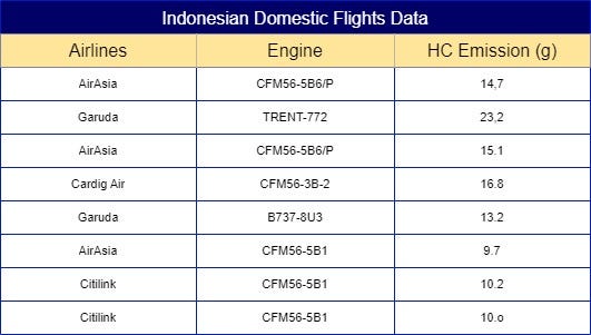
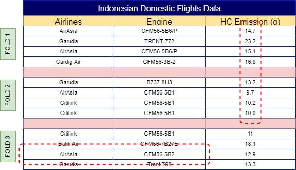
Fig 1. Indonesian Domestic Flights Dataset [1]
Using an example from Fig 1. of a sample dataset of Indonesian domestic flights emissions for each flight cycle, we can put this technique into practice. The base question to ask with this dataset is “What is the weighted mean for each categorical labels in ‘Airlines’ by looking at feature ‘HC Emission’ ?”. However, you might come with the same question people been asking me about. “But, if you just calculated them using the targeted feature, couldn’t it result as another high cardinality feature?”. The simple answer is “Yes, it could”.
Why?
In cases where a large dataset has a highly random target feature without identifiable patterns, K-Fold Target Encoding might produce a wide variety of mean values for each categorical label, potentially preserving high cardinality rather than reducing it. However, the primary goal of K-Fold Target Encoding is to address high cardinality, not necessarily to reduce it drastically. This method works best when there is a meaningful correlation between the target feature and segments of the data within each categorical label.
How does K-Fold Target Encoding operate? The simplest way to explain this is that, in each fold, you calculate the mean of the target feature from the other folds. This approach provides each categorical label with a unique weight, represented as a numerical value, making it more informative. Let’s look at an example calculation using our dataset for a clearer understanding.
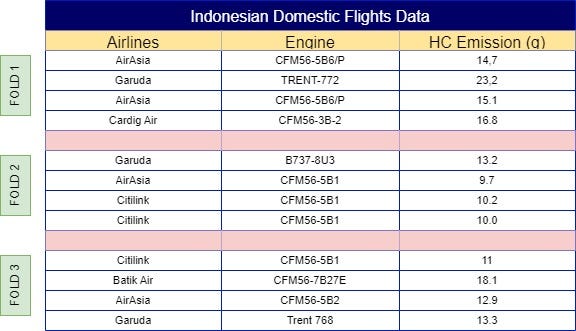
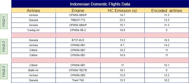
Fig 2. Indonesian Domestic Flights Dataset After K-Fold Assigned [1]
To calculate the weight of the ‘AirAsia’ label for the first observation, start by splitting the data into multiple folds, as shown in Fig 2. You can assign folds manually to ensure equal distribution, or automate this process using the following sample code:
import seaborn as sns import matplotlib.pyplot as plt
# In order to split our data into several parts equally lets assign KFold numbers to each of the data randomly.
# Calculate the number of samples per fold num_samples = len(df) // 8
# Handle any remaining samples (if len(df) is not divisible by 8) remaining_samples = len(df) % 8 if remaining_samples > 0: df.loc[-remaining_samples:, 'kfold'] = np.arange(1, remaining_samples + 1)
# Shuffle again to ensure randomness fold_df = df.sample(frac=1, random_state=42).reset_index(drop=True)
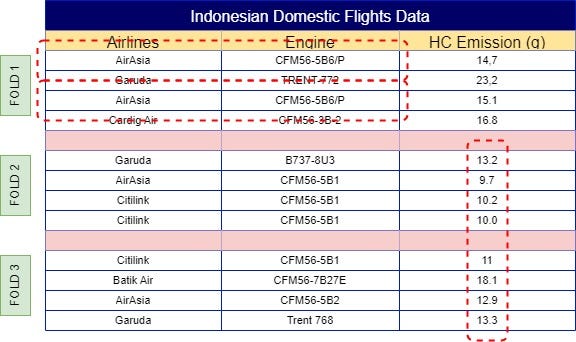
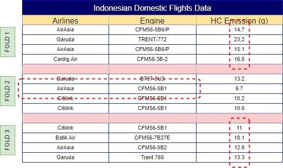
Fig 3. Category-Specific Mean Calculation Process [1]
With your dataset now split into folds, the next step is to calculate the mean of the same label across other folds. For example, ‘AirAsia’ in Fold 1 would use the mean from Folds 2, 3, 4, 5, 6, and so on, resulting in a mean of 11.3. This process continues across all folds, so Fold 2 would incorporate the mean from Folds 1, 3, 4, 5, 6, etc. The final results of these calculations are illustrated in Fig 4.
This calculation is known as the “category-specific mean,” which defines the average value for each categorical label based on similar label instances. Another essential calculation is the “global mean,” which defines the average intensity of your categorical label based on a user-defined global mean weight. The global mean serves as a baseline or “neutral” encoding, especially valuable for rare categories where the category-specific mean may rely on limited data points.
In K-Fold Target Encoding, both the category-specific and global means are typically combined to create a more robust and comprehensive representation. For a detailed illustration, refer to Fig 5.
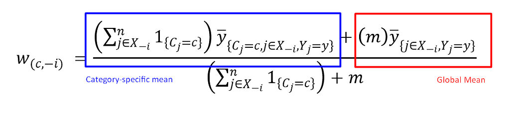
Fig 5. Mathematical Form of K-Fold Target Encoder. [1]
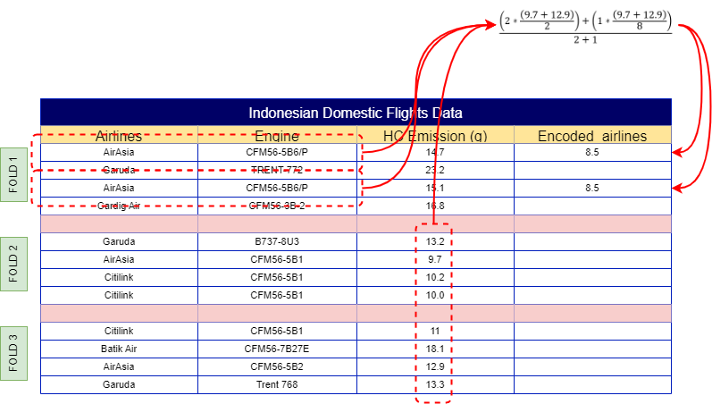
The mathematical formula makes it easier to understand how this calculation works. Here, m represents a user-defined weight, allowing control over the influence of the global mean in the final calculation. Now, we can apply this formula to the dataset from Fig 2 and implement it using the code below.
Fig 6. K-Fold Target Encoding Process Using Both Means. [1]
# First we have to encode the categorical features using K-Fold target encoding
def useful_feature(df, target, weight): utilized_feature = [c for c in df.columns if c not in (target)] obj = [col for col in df.columns if df[col].dtype == 'object'] global_mean = df[target].mean()
for objek in obj: df[f"countperobject_{objek}"] = 0 df[f"meanperobject_{objek}"] = 0
counts = agg['count'].values mean = agg['mean'].values
# Iterate over each row for i in range(1, 9): # design regarding to the length of the k-fold for index, row in df.iterrows():
# Get the category and target value if row["kfold"] != i: category = row[objek] target_val = row[target]
# Get the count from agg count_agg = agg[(agg[objek] == category)]['count'].values if len(count_agg) > 0: df.at[index, f"countperobject_{objek}"] = count_agg[0]
# Get the mean from agg mean_agg = agg[(agg[objek] == category)]['mean'].values if len(mean_agg) > 0: df.at[index, f"meanperobject_{objek}"] = mean_agg[0]
# Now find the weighted mean df[f"weightedmean_{objek}"] = ((df[f"countperobject_{objek}"] * df[f"meanperobject_{objek}"]) + (weight * global_mean))/(weight + df[f"countperobject_{objek}"])
encoding_maps = {} for objek in obj: encoding_maps[objek] = df.groupby(objek)[[f"countperobject_{objek}", f"meanperobject_{objek}"]].mean().to_dict()
return df, encoding_maps
Now with plotting the same formula into each of the categorical labels, the outcome would look like Fig 7.
Fig 7. K-Fold Target Encoding Final Result (Both Means). [1]
It’s important to remember that this method can be risky if there is a significant difference between your training and test datasets. For example, if AirAsia consistently produces high volumes of HC emissions in your training data, but in your test data, Garuda has the highest HC emissions distributed evenly, the model may overfit to the training pattern, leading to lower accuracy on new data.
Thanks for reading this article, hope you can get a better view of what is K-Fold Target Encoding and when to use it. Go check out my social media here and help me grow a better community for future data talents!!!:
A dive into the isolation forest model to detect anomalies in time-series data
Anomaly detection is a must-have capability for any organization. By detecting anomalies and outliers, we not only identify data that seems suspicious (or possibly wrong), but can also establish what ‘normal’ data looks like. Anomaly detection can prove to be a vital capability for a strong data governance system by identifying data errors. And for analysis, outliers can be a point of interest in certain cases such as fraud detection and predictive maintenance.
However, as data grows, anomaly detection can prove more and more difficult. High-dimensional data comes with noise and makes it difficult to use for analysis and insights. Large datasets are also likely to have errors and/or special cases. Thankfully, ensemble learning brings speed and efficiency to help us wrangle high-dimensional data and detect anomalies.
What is ensemble learning?
Ensemble learning is a machine learning technique that combines the predictions from multiple individual models to obtain a better predictive performance than any single model. Each model is considered a “weak learner” and is trained on a small subset of the data to make a prediction. Then it goes to a vote. Each weak learner is surveyed and the majority vote wins for the final prediction.
Ensemble models (trained on high-quality data) are robust, accurate, efficient, and are good at avoiding overfitting. They have many use cases such as classification, optimization, and in our case, anomaly detection.
The Isolation Forest Model
The isolation forest model is an ensemble of trees that isolates observations that are few and far between. It is very similar to the popular ‘Random Forest’ model, but instead of a forest of decision trees, the isolation forest produces a forest of ‘isolation trees’.
So how does it work? Let’s look at one isolation tree.
Image by the author
Consider the data above. We can see that one data point is farther away from the rest of the data (our suspected anomaly). Each isolation tree randomly chooses a ‘split value’ to begin to isolate observations. In this case, the suspected outlier is immediately isolated. This would be the case for most of the isolation trees due to its distance from the rest of the data.
Image by the author
Next, it chooses another split. This time, the suspected ‘normal’ data begins to get cut up. This process repeats until each observation is isolated. Ultimately, the model ‘isolates’ observations by randomly selecting a feature and then randomly selecting a split value between the maximum and minimum values of the selected feature.
Image by the author
Now that each observation is isolated, we need to ask: How many splits did it take for each observation to be isolated? In other words, how long is the partition path for each data point? Let’s say the results are the following:
Image by the author
Now that we know how many splits it took to isolate each observation, we calculate the mean number of splits. In our example, on average, it takes 2.6 splits to isolate an observation. Observations that have a noticeably shorter partition path, or took noticeably less splits to be isolated, are highly likely to be anomalies or outliers. The degree to which they differ from the mean number of splits is a parameter in the model. Finally, the isolation tree determines the observation G is an anomaly.
The last step of the isolation forest model is for each isolation tree to ‘vote’ on which observations are anomalies. If a majority of them think that observation G is an anomaly, then the model determines that it is.
Detecting Anomalies in Time Series Data
Lets see a simple example using the isolation forest model to detect anomalies in time-series data. Below, we have imported a sales data set that contains the day of an order, information about the product, geographical information about the customer, and the amount of the sale. To keep this example simple, lets just look at one feature (sales) over time.
#packages for data manipulation
import pandas as pd
from datetime import datetime

#packages for modeling
from sklearn.ensemble import IsolationForest

#packages for data visualization
import matplotlib.pyplot as plt
#import sales data
sales = pd.read_excel("Data/Sales Data.xlsx")

#subset to date and sales
revenue = sales[['Order Date', 'Sales']]
revenue.head()
Image by the author
As you can see above, we have the total sale amount for every order on a particular day. Since we have a sufficient amount of data (4 years worth), let’s try to detect months where the total sales is either noticeably higher or lower than the expected total sales.
First, we need to conduct some preprocessing, and sum the sales for every month. Then, visualize monthly sales.
#format the order date to datetime month and year
revenue['Order Date'] = pd.to_datetime(revenue['Order Date'],format='%Y-%m').dt.to_period('M')

#sum sales by month and year
revenue = revenue.groupby(revenue['Order Date']).sum()

#set date as index
revenue.index = revenue.index.strftime('%m-%Y')
#set the fig size
plt.figure(figsize=(8, 5))

#create the line chart
plt.plot(revenue['Order Date'],
         revenue['Sales'])

#add labels and a title
plt.xlabel('Moth')
plt.ylabel('Total Sales')
plt.title('Monthly Sales')

#rotate x-axis labels by 45 degrees for better visibility
plt.xticks(rotation = 90)

#display the chart
plt.show()
Image by the author
Using the line chart above, we can see that while sales fluctuates from month-to-month, total sales trends upward over time. Ideally, our model will identify months where total sales fluctuates more that expected and is highly influential to our overall trend.
Now we need to initialize and fit our model. The model below uses the default parameters. I have highlighted these parameters as they are the most important to the model’s performance.
n_estimators: The number of base estimators in the ensemble.
max_samples: The number of samples to draw from X to train each base estimator (if “auto”, then max_samples = min(256, n_samples)).
contamination: The amount of contamination of the data set, i.e. the proportion of outliers in the data set. Used when fitting to define the threshold on the scores of the samples.
max_features: The number of features to draw from X to train each base estimator.
#set isolation forest model and fit to the sales
model = IsolationForest(n_estimators = 100, max_samples = 'auto', contamination = float(0.1), max_features = 1.0)
model.fit(revenue[['Sales']])
Next, lets use the model to display the anomalies and their anomaly score. The anomaly score is the mean measure of normality of an observation among the base estimators. The lower the score, the more abnormal the observation. Negative scores represent outliers, positive scores represent inliers.
Lastly, lets bring up the same line chart from before, but highlighting the anomalies with plt.scatter.
Image by the author
The model appears to do well. Since the data fluctuates so much month-to-month, a worry could be that inliers would get marked as anomalies, but this is not the case due to the bootstrap sampling of the model. The anomalies appear to be the larger fluctuations where sales deviated from the trend a ‘significant’ amount.
However, knowing the data is important here as some of the anomalies should come with a caveat. Let’s look at the first (February 2015) and last (November 2018) anomaly detected. At first, we see that they both are large fluctuations from the mean.
However, the first anomaly (February 2015) is only our second month of recording sales and the business may have just started operating. Sales are definitely low, and we see a large spike the next month. But is it fair to mark the second month of business an anomaly because sales were low? Or is this the norm for a new business?
For our last anomaly (November 2018), we see a huge spike in sales that appears to deviate from the overall trend. However, we have run out of data. As data continues to be recorded, it may not have been an anomaly, but perhaps an identifier of a steeper upwards trend.
Conclusion
In conclusion, anomaly detection is a must-have capability for both strong data governance and rigorous analysis. While detecting outliers and anomalies in large data can be difficult, ensemble learning methods can help as they are robust and efficient with large, tabular data.
The isolation forest model detects these anomalies by for using a forest of ‘weak learners’ to isolate observations that are few and far between.
I hope you have enjoyed my article! Please feel free to comment, ask questions, or request other topics.
The Ultimate Guide to RAGs — Each Component Dissected
A visual tour of what it takes to build CHAD-level LLM pipelines
Let’s learn RAGs! (Image by Author)
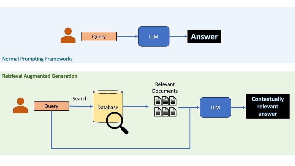
If you have worked with Large Language Models, there is a great chance that you have at least heard the term RAG — Retrieval Augmented Generation. The idea of RAGs are pretty simple — suppose you want to ask a question to a LLM, instead of just relying on the LLM’s pre-trained knowledge, you first retrieve relevant information from an external knowledge base. This retrieved information is then provided to the LLM along with the question, allowing it to generate a more informed and up-to-date response.
Comparing standard LLM calls with RAG (Source: Image by Author)
So, why use Retrieval Augmented Generation?
When providing accurate and up-to-date information is key, you cannot rely on the LLM’s inbuilt knowledge. RAGs are a cheap practical way to use LLMs to generate content about recent topics or niche topics without needing to finetune them on your own and burn away your life’s savings. Even when LLMs internal knowledge may be enough to answer questions, it might be a good idea to use RAGs anyway, since recent studies have shown that they could help reduce LLMs hallucinations.
The different components of a bare-bones RAG
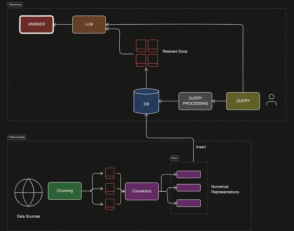
Before we dive into the advanced portion of this article, let’s review the basics. Generally RAGs consist of two pipelines — preprocessing and inferencing.
Inferencing is all about using data from your existing database to answer questions from a user query. Preprocessing is the process of setting up the database in the correct way so that retrieval is done correctly later on.
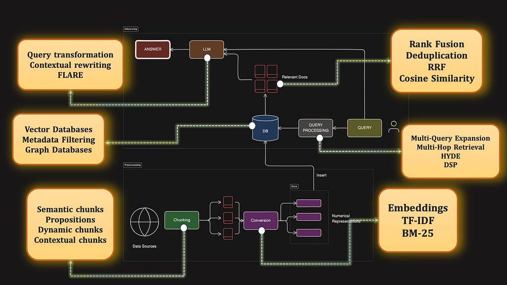
Here is a diagramatic look into the entire basic barebones RAG pipeline.
The Basic RAG pipeline (Image by Author)
The Indexing or Preprocessing Steps
This is the offline preprocessing stage, where we would set up our database.
Identify Data Source: Choose a relevant data source based on the application, such as Wikipedia, books, or manuals. Since this is domain dependent, I am going to skip over this step in this article. Go choose any data you want to use, knock yourself out!
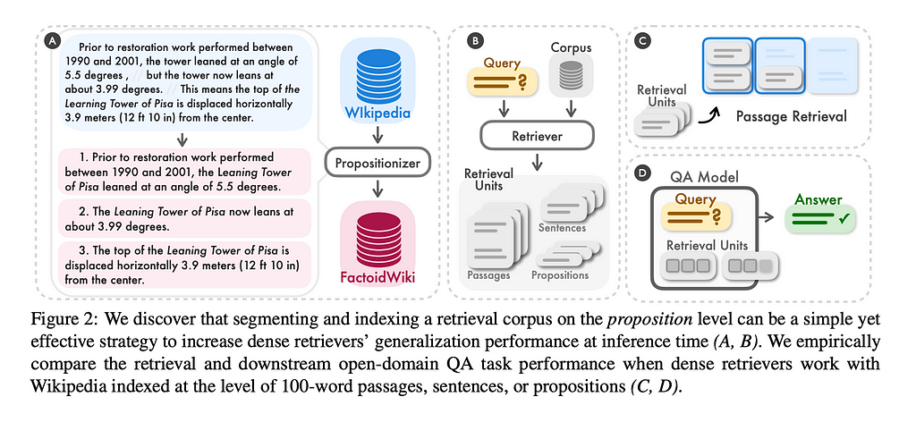
Chunking the Data: Break down the dataset into smaller, manageable documents or chunks.
Convert to Searchable Format: Transform each chunk into a numerical vector or similar searchable representation.
Insert into Database: Store these searchable chunks in a custom database, though external databases or search engines could also be used.
The Inferencing Steps
During the Query Inferencing stage, the following components stand out.
Query Processing: A method to convert the user’s query into a format suitable for search.
Retrieval/Search Strategy: A similarity search mechanism to retrieve the most relevant documents.
Post-Retrieval Answer Generation: Use retrieved documents as context to generate the answer with an LLM.
Great — so we identified several key modules required to build a RAG. Believe it or not, each of these components have a lot of additional research to make this simple RAG turn into CHAD-rag. Let’s look into each of the major components in this list, starting with chunking.
By the way, this article is based on this 17-minute Youtube video I made on the same topic, covering all the topics in this article. Feel free to check it out after reading this Medium article!
1. Chunking
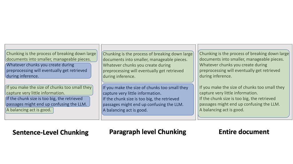
Chunking is the process of breaking down large documents into smaller, manageable pieces. It might sound simple, but trust me, the way you chunk your data can make or break your RAG pipeline. Whatever chunks you create during preprocessing will eventually get retrieved during inference. If you make the size of chunks too small — like each sentence — then it might be difficult to retrieve them through search because they capture very little information. If the chunk size is too big — like inserting entire Wikipedia articles — the retrieved passages might end up confusing the LLM because you are sending large bodies of texts at once.
Depending on the different levels of chunking, your results may vary! (Image by author)
Some frameworks use LLMs to do chunking, for example by extracting simple factoids or propositions from the text corpus, and treat them as documents. This could be expensive because the larger your dataset, the more LLM calls you’ll have to make.
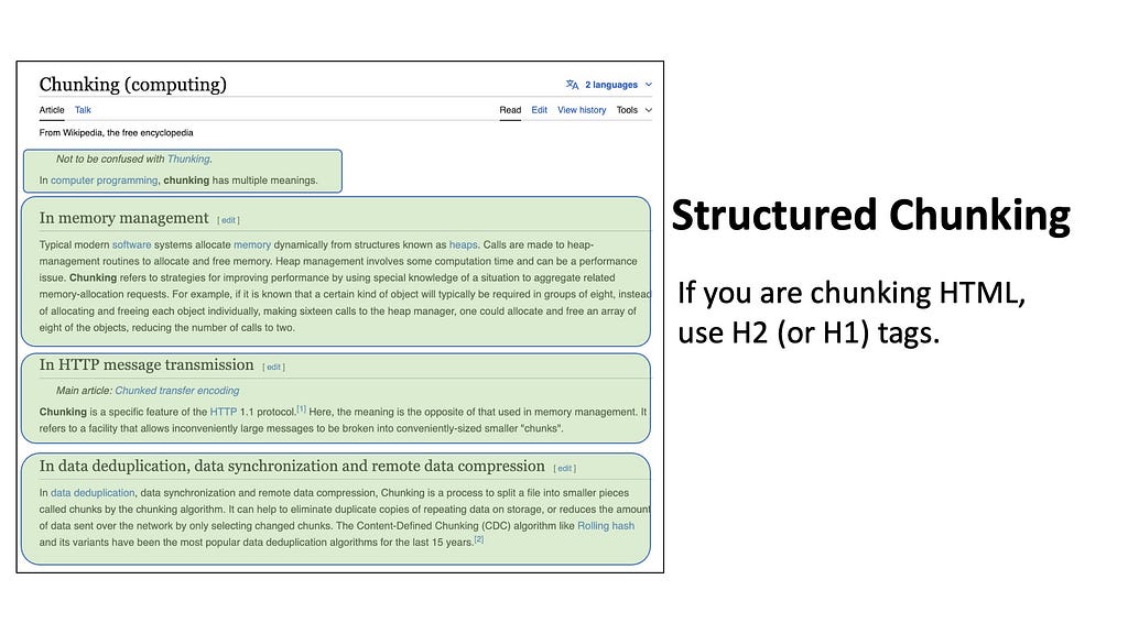
If your data has inherent boundaries (like HTML or Code), sometimes it is best to just utilize it. (Image by Author)
Quite often we may also deal with datasets that inherently have a known structure or format. For example, if you want to insert code into your database, you can simply split each script by the function names or class definitions. For HTML pages like Wikipedia articles, you can split by the heading tags — for example, split by the H2 tags to isolate each sub-chapter.
Contextual Chunking
But there are some glaring issues with the types of chunking we have discussed so far. Suppose your dataset consists of tens of thousands of paragraphs extracted from all Sherlock Holmes books. Now the user has queried something general like what was the first crime in Study in Scarlet? What do you think is going to happen?
The problem is that since each documented is an isolated piece of information, we don’t know which chunks are from the book Study in Scarlet. Therefore, later on during retrieval, we will end up fetch a bunch of passages about the topic “crime” without knowing if it’s relevant to the book. To resolve this, we can use something known as contextual chunking.
Enter Contextual Chunking
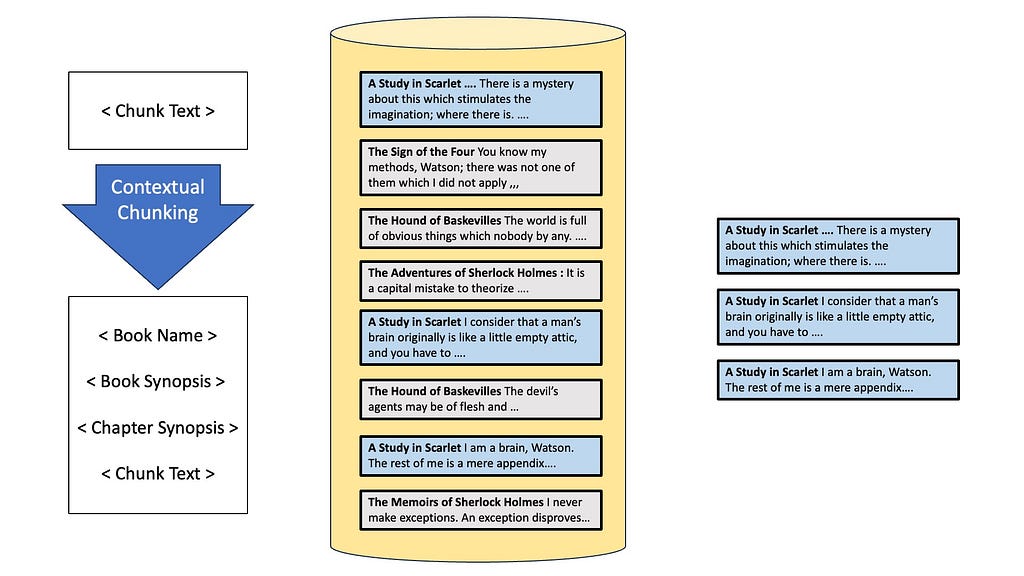
A recent blogpost from Anthropic describes it as prepending chunk-specific explanatory context to each chunk before embedding. Basically, while we are indexing, we would also include additional information relevant to the chunk — like the name of the book, the chapter, maybe a summary of the events in the book. Adding this context will allow the retriever to find references to Study in Scarlett and crimes when searching, hopefully getting the right documents from the database!
Contextual Chunking adds additional information to the chunks than just the text body (Image by author)
There are other ways to solve the problem of finding the right queries — like metadata filtering, We will talk about this later when we talk about Databases.
2. Data Conversion
Next, we come to the data-conversion stage. Note that whatever strategy we used to convert the documents during preprocessing, we need to use it to search for similarity later, so these two components are tightly coupled.
Two of the most common approaches that have emerged in this space are embedding based methods and keyword-frequency based methods like TF-IDF or BM-25.
Embedding Based Methods
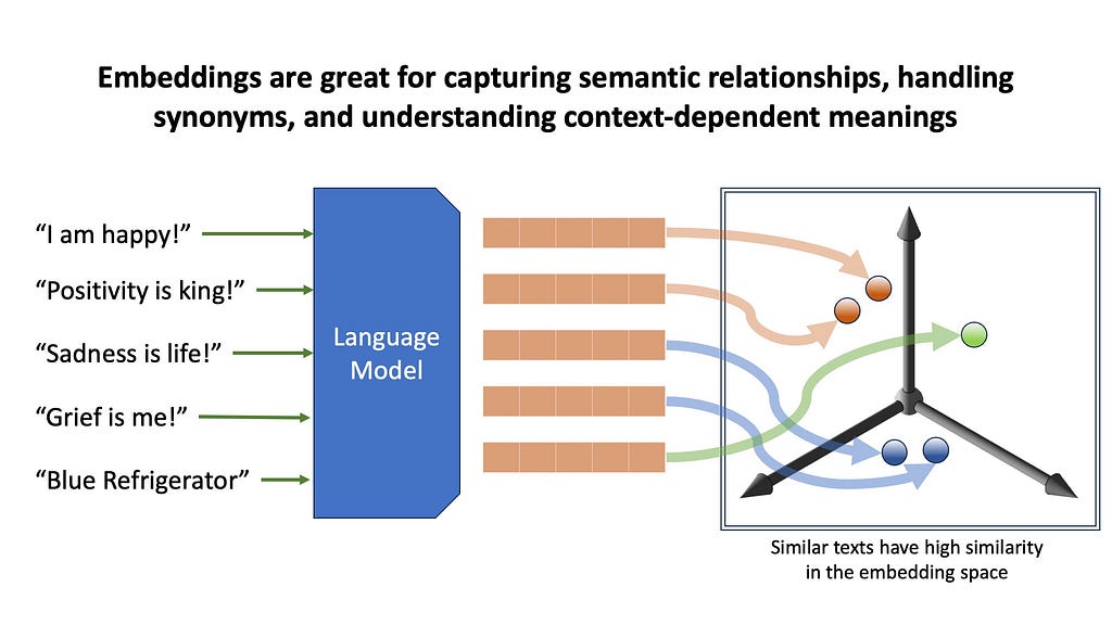
We’ll start with embedding-based methods. Here, we use pretrained transformer models to transform the text into high-dimensional vector representations, capturing semantic meaning about the text. Embeddings are great for capturing semantic relationships, handling synonyms, and understanding context-dependent meanings. However, embedding can be computationally intensive, and can sometimes overlook exact matches that simpler methods would easily catch.
Embeddings (Image by Author)
When does Semantic Search fail?
For example, suppose you have a database of manuals containing information about specific refrigerators. When you ask a query mentioning a very specific niche model or a serial number, embeddings will fetch documents that kind of resemble your query, but may fail to exactly match it. This brings us to the alternative of embeddings retrieval — keyword based retrieval.
Keyword Based Methods
Two popular keyword-based methods are TF-IDF and BM25. These algorithms focus on statistical relationships between terms in documents and queries.
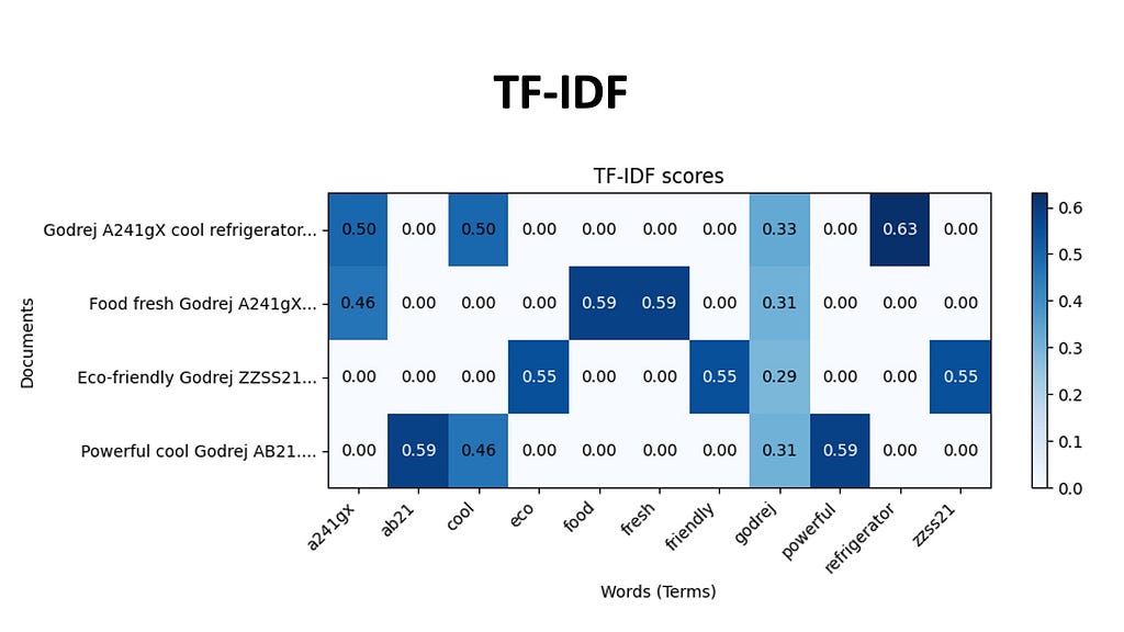
TF-IDF weighs the importance of a word based on its frequency in a document relative to its frequency in the entire corpus. Every document in our dataset is be represented by a array of TF-IDF scores for each word in the vocabulary. The indices of the high values in this document vector tell us which words that are likely to be most characteristic of that document’s content, because these words appear more frequently in this document and less frequently in others. For example, the documents related to this Godrej A241gX , will have a high TF-IDF score for the phrase Godrej and A241gX, making it more likely for us to retrieve this using TF-IDF.
TF-IDF relies on the ratio of the occurence of terms in a document compared to the entire corpus. (Image by author)
BM25, an evolution of TF-IDF, incorporates document length normalization and term saturation. Meaning that it adjusts the TF-IDF score based on if the document itself is longer or shorter than the average document length in the collection. Term saturation means that as a particular word appears too often in the database, it’s importance decreases.
TF-IDF and BM-25 are great finding documents with specific keyword occurrences when they exactly occur. And embeddings are great for finding documents with similar semantic meaning.
A common thing these days is to retrieve using both keyword and embedding based methods, and combine them, giving us the best of both worlds. Later on when we discuss Reciprocal Rank Fusion and Deduplication, we will look into how to combine these different retrieval methods.
3. Databases
Up next, let’s talk about Databases. The most common type of database that is used in RAGs are Vector Databases. Vector databases store documents by indexing them with their vector representation, be in from an embedding, or TF-IDF. Vector databases specialize in fast similarity check with query vectors, making them ideal for RAG. Popular vector databases that you may want to look into are Pinecone, Milvus, ChromaDB, MongoDB, and they all have their pros and cons and pricing model.
An alternative to vector databases are graph databases. Graph databases store information as a network of documents with each document connected to others through relationships.
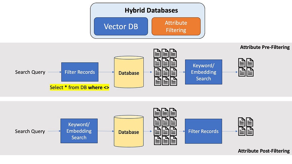
Modern Vector Databases allow attribute filtering with semantic search (Image by Author)
Many modern vector and graph database also allow properties from relational databases, most notably metadata or attribute filtering. If you know the question is about the 5th Harry Potter book, it would be really nice to filter your entire database first to only contain documents from the 5th Harry Potter book, and not run embeddings search through the entire dataset. Optimal metadata filtering in Vector Databases is a pretty amazing area in Computer Science research, and a seperate article would be best for a in-depth discussion about this.
4. Query transformation
Next, let’s move to inferencing starting with query transformation — which is any preprocessing step we do to the user’s actual query before doing any similarity search. Think of it like improving the user’s question to get better answers.
In general, we want to avoid searching directly with the user query. User inputs are usually very noisy and they can type random stuff — we want an additional transformation layer that interprets the user query and turns it into a search query.
A simple example why Query Rewriting is important
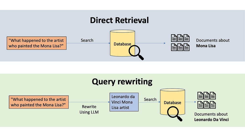
The most common technique to do this transformation is query rewriting. Imagine someone asks, “What happened to the artist who painted the Mona Lisa?” If we do semantic or keyword searches, the retrieved information will be all about the Mona Lisa, not about the artist. A query rewriting system would use an LLM to rewrite this query. The LLM might transform this into “Leonardo da Vinci Mona Lisa artist”, which will be a much fruitful search.
Direct Retrieval vs Query Rewriting (Image by Author)
Sometimes we would also use Contextual Query Writing, where we might use additional contexts, like using the older conversation transcript from the user, or if we know that our application covers documents from 10 different books, maybe we can have a classifier LLM that classifies the user query to detect which of the 10 books we are working with. If our database is in a different language, we can also translate the query.
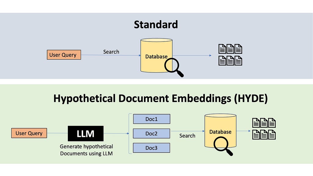
There are also powerful techniques like HYDE, which stands for Hypothetical Document Embedding. HYDE uses a language model to generate a hypothetical answer to the query, and do similarity search with this hypothetical answer to retrieve relevant documents.
Hypothetical Document Embeddings (Image by Author)
Another technique is Multi-Query Expansion where we generate multiple queries from the single user query and perform parallel searches to retrieve multiple sets of documents. The received documents can then later go through a de-duplication step or rank fusion to remove redundant documents.
A recent approach called Astute RAGtries to consolidate externally input knowledge with the LLM’s own internal knowledge before generating answers. There are also Multi-Hop techniques like Baleen programs. They work by performing an initial search, analyzing the top results to find frequently co-occurring terms, and then adding these terms to the original query. This adaptive approach can help bridge the vocabulary gap between user queries and document content, and help retrieve better documents.
5. Post Retrieval Processing
Now that we’ve retrieved our potentially relevant documents, we can add another post-retrieval processing step before feeding information to our language model for generating the answer.
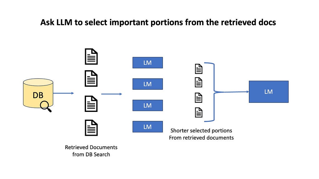
For example, we can do information selection and emphasis, where an LLM selects portion of the retrieved documents that could be useful for finding the answer. We might highlight key sentences, or do semantic filtering where we remove unimportant paragraphs, or do context summarization by fusing multiple documents into one. The goal here is to avoid overwhelming our LLM with too much information, which could lead to less focused or accurate responses.
You can use smaller LLMs to flag relevant info from retrieved documents before consolidating the context prompt for the final LLM call (Image by Author)
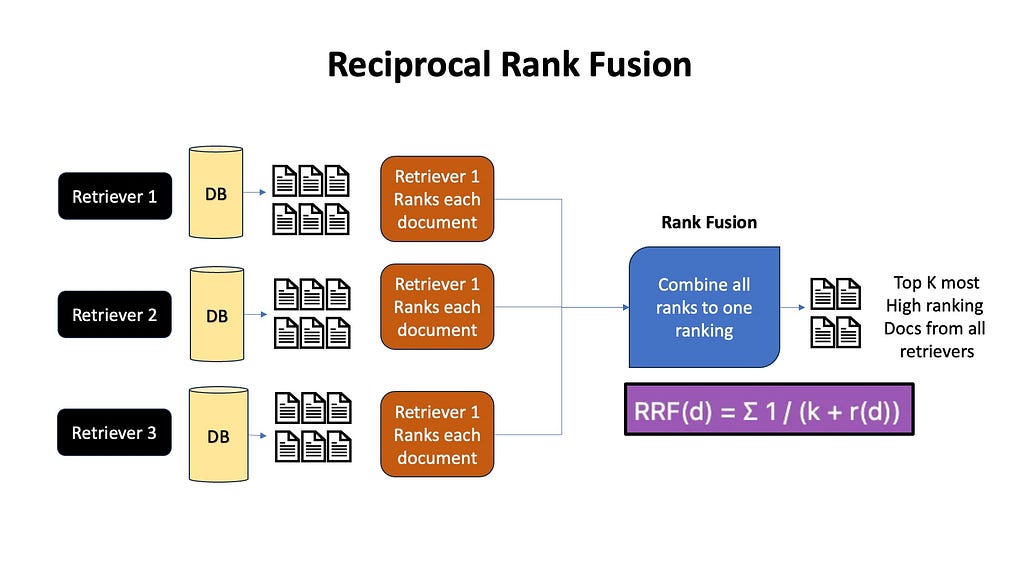
Often we do multiple queries with query expansion, or use multiple retrieval algorithms like Embeddings+BM-25 to separately fetch multiple documents. To remove duplicates, we often use reranking methods like Reciprocal Rank Fusion. RRF combines the rankings from all the different approaches, giving higher weight to documents that consistently rank well across multiple methods. In the end, the top K high ranking documents are passed to the LLM.
Reciprocal Rank Fusion is a classic Search Engine algorithm to combine item ranks obtained from multiple ranking algorithms (Image by author)
FLARE or forward-looking active retrieval augmented generation is an iterative post-retrieval strategy. Starting with the user input and initial retrieval results, an LLM iteratively guesses the next sentence. Then we check if the generated guess contains any low probability tokens indicated here with an underline — if so, we call the retriever to retrieve useful documents from the dataset and make necessary corrections.
Final Thoughts
For a more visual breakdown of the different components of RAGs, do checkout my Youtube video on this topic. The field of LLMs and RAGs are rapidly evolving — a thorough understanding of the RAG framework is incredibly essential to appreciate the pros and cons of each approach and weigh which approaches work best for YOUR use-case. The next time you are thinking of designing a RAG system, do stop and ask yourself these questions —
What are my data sources?
How should I chunk my data? Is there inherent structure that comes with my data domain? Do my chunks need additional context (contextual chunking)?
Do I need semantic retrieval (embeddings) or more exact-match retrieval (BM-25)? What type of queries am I expecting from the user?
What database should I use? Is my data a graph? Does it need metadata-filtering? How much money do I want to spend on databases?
How can I best rewrite the user query for easy search hits? Can an LLM rewrite the queries? Should I use HYDE? If LLMs already have enough domain knowledge about my target field, can I use Astute?
Can I combine multiple different retrieval algorithms and then do rank fusion? (honestly, just do it if you can afford it cost-wise and latency-wise)
The Author
Check out my Youtube channel where I post content about Deep Learning, Machine Learning, Paper Reviews, Tutorials, and just about anything related to AI (except news, there are WAY too many Youtube channels for AI news). Here are some of my links:
We use cookies on our website to give you the most relevant experience by remembering your preferences and repeat visits. By clicking “Accept”, you consent to the use of ALL the cookies.
This website uses cookies to improve your experience while you navigate through the website. Out of these, the cookies that are categorized as necessary are stored on your browser as they are essential for the working of basic functionalities of the website. We also use third-party cookies that help us analyze and understand how you use this website. These cookies will be stored in your browser only with your consent. You also have the option to opt-out of these cookies. But opting out of some of these cookies may affect your browsing experience.
Necessary cookies are absolutely essential for the website to function properly. These cookies ensure basic functionalities and security features of the website, anonymously.
Cookie
Duration
Description
cookielawinfo-checkbox-analytics
11 months
This cookie is set by GDPR Cookie Consent plugin. The cookie is used to store the user consent for the cookies in the category "Analytics".
cookielawinfo-checkbox-functional
11 months
The cookie is set by GDPR cookie consent to record the user consent for the cookies in the category "Functional".
cookielawinfo-checkbox-necessary
11 months
This cookie is set by GDPR Cookie Consent plugin. The cookies is used to store the user consent for the cookies in the category "Necessary".
cookielawinfo-checkbox-others
11 months
This cookie is set by GDPR Cookie Consent plugin. The cookie is used to store the user consent for the cookies in the category "Other.
cookielawinfo-checkbox-performance
11 months
This cookie is set by GDPR Cookie Consent plugin. The cookie is used to store the user consent for the cookies in the category "Performance".
viewed_cookie_policy
11 months
The cookie is set by the GDPR Cookie Consent plugin and is used to store whether or not user has consented to the use of cookies. It does not store any personal data.
Functional cookies help to perform certain functionalities like sharing the content of the website on social media platforms, collect feedbacks, and other third-party features.
Performance cookies are used to understand and analyze the key performance indexes of the website which helps in delivering a better user experience for the visitors.
Analytical cookies are used to understand how visitors interact with the website. These cookies help provide information on metrics the number of visitors, bounce rate, traffic source, etc.
Advertisement cookies are used to provide visitors with relevant ads and marketing campaigns. These cookies track visitors across websites and collect information to provide customized ads.


