A step-by-step guide on getting the most of lengthy data reports, within seconds
Originally appeared here:
Python Might Be Your Best PDF Data Extractor
Go Here to Read this Fast! Python Might Be Your Best PDF Data Extractor
A step-by-step guide on getting the most of lengthy data reports, within seconds
Originally appeared here:
Python Might Be Your Best PDF Data Extractor
Go Here to Read this Fast! Python Might Be Your Best PDF Data Extractor
Business documents, such as complex reports, product catalogs, design files, financial statements, technical manuals, and market analysis reports, usually contain multimodal data (text as well as visual content such as graphs, charts, maps, photos, infographics, diagrams, and blueprints, etc.). Finding the right information from these documents requires a semantic search of text and related images for a given query posed by a customer or a company employee. For instance, a company’s product might be described through its title, textual description, and images. Similarly, a project proposal might include a combination of text, charts illustrating budget allocations, maps showing geographical coverage, and photos of past projects.
Accurate and quick search of multimodal information is important for improving business productivity. Business data is often spread across various sources in text and image formats, making retrieving all relevant information efficiently challenging. While generative AI methods, particularly those leveraging LLMs, enhance knowledge management in business (e.g., retrieval augment generation, graph RAGs, among others), they face limitations in accessing multimodal, scattered data. Methods that unify different data types allow users to query diverse formats with natural language prompts. This capability can benefit employees and management within a company and improve customer experience. It can have several use cases, such as clustering similar topics and discovering thematic trends, building recommendation engines, engaging customers with more relevant content, faster access to information for improved decision-making, delivering user-specific search results, enhancing user interactions to feel more intuitive and natural, and reducing time spent finding information, to name a few.
In modern AI models, data is processed as numerical vectors known as embeddings. Specialized AI models, called embedding models, transform data into numerical representations that can be used to capture and compare similarities in meaning or features efficiently. Embeddings are extremely useful for semantic search and knowledge mapping and serve as the foundational backbone of today’s sophisticated LLMs.
This article explores the potential of embedding models (particularly multimodal embedding models introduced later) for enhancing semantic search across multiple data types in business applications. The article begins by explaining the concept of embeddings for readers unfamiliar with how embeddings work in AI. It then discusses the concept of multimodal embeddings, explaining how the data from multiple data formats can be combined into unified embeddings that capture cross-modal relationships and could be immensely useful for business-related information search tasks. Finally, the article explores a recently introduced multimodal embedding model for multimodal semantic search for business applications.
Embeddings are stored in a vector space where similar concepts are located close to each other. Imagine the embedding space as a library where books on related topics are shelved together. For example, in an embedding space, embeddings for words like “desk” and “chair” would be near to each other, while “airplane” and “baseball” would be further apart. This spatial arrangement enables models to identify and retrieve related items effectively and enhances several tasks like recommendation, search, and clustering.
To demonstrate how embeddings are computed and visualized, let’s create some categories of different concepts. The complete code is available on GitHub.
categories = {
    "Fruits": ["Apple", "Banana", "Orange", "Grape", "Mango", "Peach", "Pineapple"],
    "Animals": ["Dog", "Cat", "Elephant", "Tiger", "Lion", "Monkey", "Rabbit"],
    "Countries": ["Canada", "France", "India", "Japan", "Brazil", "Germany", "Australia"],
    "Sports": ["Soccer", "Basketball", "Tennis", "Baseball", "Cricket", "Swimming", "Running"],
    "Music Genres": ["Rock", "Jazz", "Classical", "Hip Hop", "Pop",  "Blues"],
    "Professions": ["Doctor", "Engineer", "Teacher", "Artist", "Chef", "Lawyer", "Pilot"],
    "Vehicles": ["Car", "Bicycle", "Motorcycle", "Airplane", "Train", "Boat", "Bus"],
    "Furniture": ["Chair", "Table", "Sofa", "Bed", "Desk", "Bookshelf", "Cabinet"],
    "Emotions": ["Happiness", "Sadness", "Anger", "Fear", "Surprise", "Disgust", "Calm"],
    "Weather": ["Hurricane", "Tornado", "Blizzard", "Heatwave", "Thunderstorm", "Fog"],
    "Cooking": ["Grilling", "Boiling", "Frying", "Baking", "Steaming", "Roasting", "Poaching"]

}
I will now use an embedding model (Cohere’s embed-english-v3.0 model which is the focus of this article and will be discussed in detail after this example) to compute the embeddings of these concepts, as shown in the following code snippet. The following libraries need to be installed for running this code.
!pip install cohere umap-learn seaborn matplotlib numpy pandas regex altair scikit-learn ipython faiss-cpu
This code computes the text embeddings of the above-mentioned concepts and stores them in a NumPy array.
import cohere
import umap
import seaborn as sns
import matplotlib.pyplot as plt
import numpy as np
import pandas as pd

# Initialize Cohere client
co = cohere.Client(api_key=os.getenv("COHERE_API_KEY_2"))
# Flatten categories and concepts
labels = []
concepts = []
for category, items in categories.items():
    labels.extend([category] * len(items))
    concepts.extend(items)

# Generate text embeddings for all concepts with corrected input_type
embeddings = co.embed(
    texts=concepts,
    model="embed-english-v3.0",
    input_type="search_document"  # Corrected input type for text
).embeddings

# Convert to NumPy array
embeddings = np.array(embeddings)
Embeddings can have hundreds or thousands of dimensions that are not possible to visualize directly. Hence, we reduce the dimensionality of embeddings to make high-dimensional data visually interpretable. After computing the embeddings, the following code maps the embeddings to a 2-dimensional space using the UMAP (Uniform Manifold Approximation and Projection) dimensionality reduction method so that we can plot and analyze how similar concepts cluster together.
# Dimensionality reduction using UMAP
reducer = umap.UMAP(n_neighbors=20, random_state=42)
reduced_embeddings = reducer.fit_transform(embeddings)

# Create DataFrame for visualization
df = pd.DataFrame({
    "x": reduced_embeddings[:, 0],
    "y": reduced_embeddings[:, 1],
    "Category": labels,
    "Concept": concepts
})

# Plot using Seaborn
plt.figure(figsize=(12, 8))
sns.scatterplot(data=df, x="x", y="y", hue="Category", style="Category", palette="Set2", s=100)

# Add labels to each point
for i in range(df.shape[0]):
    plt.text(df["x"][i] + 0.02, df["y"][i] + 0.02, df["Concept"][i], fontsize=9)

plt.legend(loc="lower right")
plt.title("Visualization of Embeddings by Category")
plt.xlabel("UMAP Dimension 1")
plt.ylabel("UMAP Dimension 2")
plt.savefig("C:/Users/h02317/Downloads/embeddings.png",dpi=600)

plt.show()
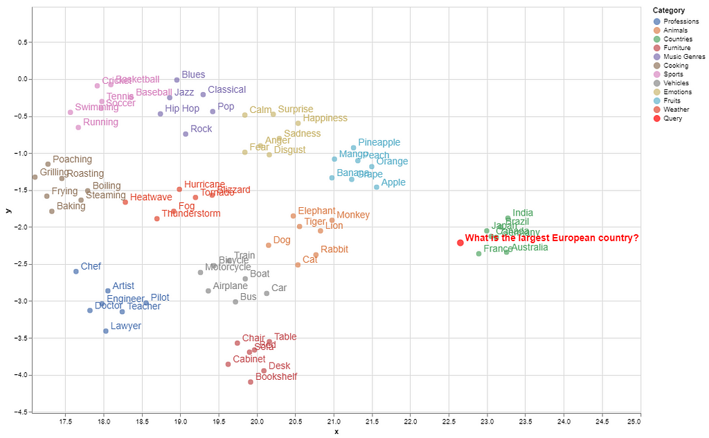
Here is the visualization of the embeddings of these concepts in a 2D space.
Semantically similar items are grouped in the embedding space, while concepts with distant meanings are located farther apart (e.g., countries are clustered farther from other categories).
To illustrate how a search query maps to its matching concept within this space, we first store the embeddings in a vector database (FAISS vector store). Next, we compute the query’s embeddings in the same way and identify a “neighborhood” in the embedding space where embeddings closely match the query’s semantics. This proximity is calculated using Euclidean distance or cosine similarity between the query embeddings and those stored in the vector database.
import cohere
import numpy as np
import re
import pandas as pd
from tqdm import tqdm
from datasets import load_dataset
import umap
import altair as alt
from sklearn.metrics.pairwise import cosine_similarity
import warnings
from IPython.display import display, Markdown
import faiss
import numpy as np
import pandas as pd
from sklearn.preprocessing import normalize
warnings.filterwarnings('ignore')
pd.set_option('display.max_colwidth', None)

# Normalize embeddings (optional but recommended for cosine similarity)
embeddings = normalize(np.array(embeddings))

# Create FAISS index
dimension = embeddings.shape[1]
index = faiss.IndexFlatL2(dimension)  # L2 distance, can use IndexFlatIP for inner product (cosine similarity)
index.add(embeddings)  # Add embeddings to the FAISS index

# Embed the query
query = "Which is the largest European country?"
query_embedding = co.embed(texts=[query], model="embed-english-v3.0", input_type="search_document").embeddings[0]
query_embedding = normalize(np.array([query_embedding]))  # Normalize query embedding

# Search for nearest neighbors
k = 5  # Number of nearest neighbors
distances, indices = index.search(query_embedding, k)

# Format and display results
results = pd.DataFrame({
    'texts': [concepts[i] for i in indices[0]],
    'distance': distances[0]
})
display(Markdown(f"Query: {query}"))
# Convert DataFrame to markdown format
def print_markdown_results(df):
    markdown_text = f"Nearest neighbors:nn"
    markdown_text += "| Texts | Distance |n"
    markdown_text += "|-------|----------|n"
    for _, row in df.iterrows():
        markdown_text += f"| {row['texts']} | {row['distance']:.4f} |n"
    display(Markdown(markdown_text))

# Display results in markdown
print_markdown_results(results)
Here are the top-5 closest matches to the query, ranked by their smallest distances from the query’s embedding among the stored concepts.
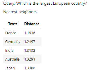
As shown, France is the correct match for this query among the given concepts. In the visualized embedding space, the query’s position falls within the ‘country’ group.
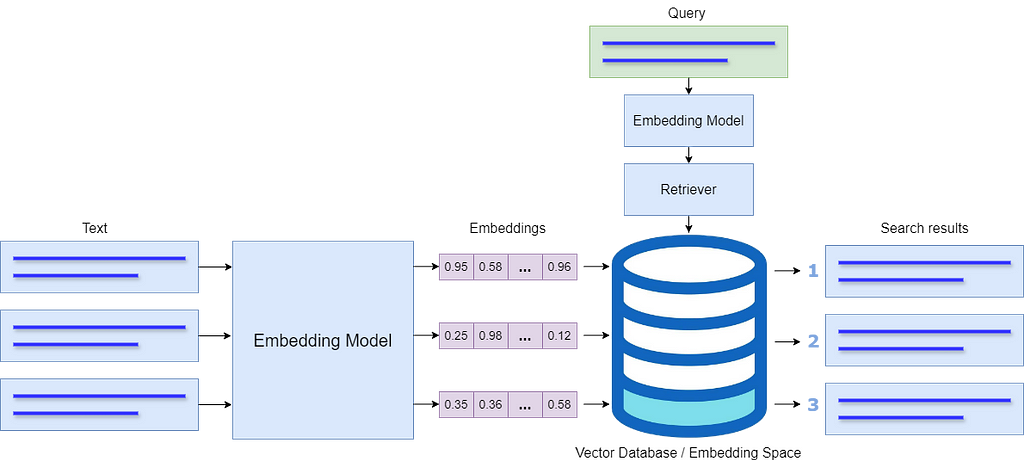
The whole process of semantic search is depicted in the following figure.
Text embeddings are successfully used for semantic search and retrieval augment generation (RAG). Several embedding models are used for this purpose, such as from OpenAI’s, Google, Cohere, and others. Similarly, several open-source models are available on the Hugging Face platform such as all-MiniLM-L6-v2. While these models are very useful for text-to-text semantic search, they cannot deal with image data which is an important source of information in business documents. Moreover, businesses often need to quickly search for relevant images either from documents or from vast image repositories without proper metadata.
This problem is partially addressed by some multimodal embedding models, such as OpenAI’s CLIP, which connects text and images and can be used to recognize a wide variety of visual concepts in images and associate them with their names. However, it has very limited text input capacity and shows low performance for text-only or even text-to-image retrieval tasks.
A combination of text and image embedding models is also used to cluster text and image data into separate spaces; however, it leads to weak search results that are biased toward text-only data. In multimodal RAGs, a combination of a text embedding model and a multimodal LLM is used to answer both from text and images. For the details of developing a multimodal RAG, please read my following article.
Integrating Multimodal Data into a Large Language Model
A multimodal embedding model should be able to include both image and text data within a single database which will reduce complexity compared to maintaining two separate databases. In this way, the model will prioritize the meaning behind data, instead of biasing towards a specific modality.
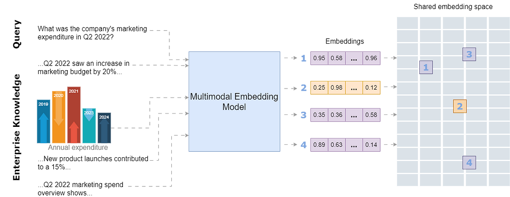
By storing all modalities in a single embedding space, the model will be able to connect text with relevant images and retrieve and compare information across different formats. This unified approach enhances search relevance and allows for a more intuitive exploration of interconnected information within the shared embedding space.
Cohere recently introduced a multimodal embedding model, Embed 3, which can generate embeddings from both text and images and store them in a unified embedding space. According to Cohere’s blog, the model shows impressive performance for a variety of multimodal tasks such as zero-shot, text-to-image, graphs and charts, eCommerce catalogs, and design files, among others.
In this article, I explore Cohere’s multimodal embedding model for text-to-image, text-to-text, and image-to-image retrieval tasks for a business scenario in which the customers search for products from an online product catalog using either text queries or images. Using text-to-image, text-to-text, and image-to-image retrieval in an online product catalog brings several advantages to businesses as well as customers. This approach allows customers to search for products in a flexible way, either by typing a query or uploading an image. For instance, a customer who sees an item they like can upload a photo, and the model will retrieve visually similar products from the catalog along with all the details about the product. Similarly, customers can search for specific products by describing their characteristics rather than using the exact product name.
The following steps are involved in this use case.
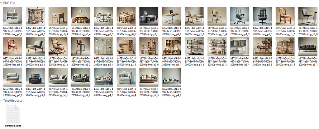
I generated an example furniture catalog of a fictitious company using OpenAI’s DALL-E image generator. The catalog comprises 4 categories of a total of 36 product images with descriptions. Here is the snapshot of the first page of the product catalog.

The complete code and the sample data are available on GitHub. Let’s discuss it step by step.
Cohere’s embedding model is used in the following way.
model_name = "embed-english-v3.0"
api_key = "COHERE_API_KEY"
input_type_embed = "search_document" #for image embeddings, input_type_embed = "image"
# Create a cohere client.
co = cohere.Client(api_key)
text = ['apple','chair','mango']
embeddings = co.embed(texts=list(text),
                  model=model_name,
                  input_type=input_type_embed).embeddings
The model can be tested using Cohere’s trial API keys by creating a free account on their website.
To demonstrate how multimodal data can be extracted, I used LlamaParse to extract product images and text from the catalog. This process is detailed in my previous article. LlamaParse can be used by creating an account on Llama Cloud website to get an API key. The free API key allows 1000 pages of credit limit per day.
The following libraries need to be installed to run the code in this article.
!pip install nest-asyncio python-dotenv llama-parse qdrant-client
The following piece of code loads the API keys of Llama Cloud, Cohere, and OpenAI from an environment file (.env). OpenAI’s multimodal LLM, GPT-4o, is used to generate the final response.
import os
import time
import nest_asyncio
from typing import List
from dotenv import load_dotenv

from llama_parse import LlamaParse
from llama_index.core.schema import ImageDocument, TextNode
from llama_index.embeddings.cohere import CohereEmbedding
from llama_index.multi_modal_llms.openai import OpenAIMultiModal
from llama_index.core import Settings
from llama_index.core.indices import MultiModalVectorStoreIndex
from llama_index.vector_stores.qdrant import QdrantVectorStore
from llama_index.core import StorageContext
import qdrant_client
from llama_index.core import SimpleDirectoryReader
# Load environment variables
load_dotenv()
nest_asyncio.apply()

# Set API keys
COHERE_API_KEY = os.getenv("COHERE_API_KEY")
LLAMA_CLOUD_API_KEY = os.getenv("LLAMA_CLOUD_API_KEY")
OPENAI_API_KEY = os.getenv("OPENAI_API_KEY")
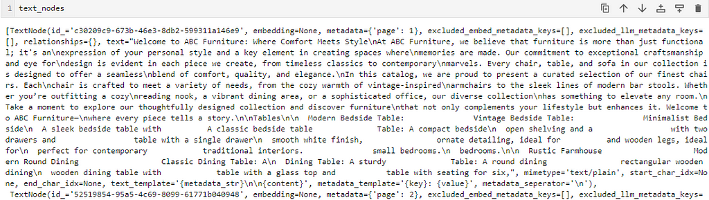
The following code extracts the text and image nodes from the catalog using LlamaParse. The extracted text and images are saved to a specified path.
# Extract text nodes
def get_text_nodes(json_list: List[dict]) -> List[TextNode]:
    return [TextNode(text=page["text"], metadata={"page": page["page"]}) for page in json_list]

# Extract image nodes
def get_image_nodes(json_objs: List[dict], download_path: str) -> List[ImageDocument]:
    image_dicts = parser.get_images(json_objs, download_path=download_path)
    return [ImageDocument(image_path=image_dict["path"]) for image_dict in image_dicts]

# Save the text in text nodes to a file
def save_texts_to_file(text_nodes, file_path):
    texts = [node.text for node in text_nodes]
    all_text = "nn".join(texts)
    with open(file_path, "w", encoding="utf-8") as file:
        file.write(all_text)

# Define file paths
FILE_NAME = "furniture.docx"
IMAGES_DOWNLOAD_PATH = "parsed_data"

# Initialize the LlamaParse parser
parser = LlamaParse(
    api_key=LLAMA_CLOUD_API_KEY,
    result_type="markdown",
)

# Parse document and extract JSON data
json_objs = parser.get_json_result(FILE_NAME)
json_list = json_objs[0]["pages"]

#get text nodes
text_nodes = get_text_nodes(json_list)

#extract the images to a specified path
image_documents = get_image_nodes(json_objs, IMAGES_DOWNLOAD_PATH)

# Save the extracted text to a .txt file
file_path = "parsed_data/extracted_texts.txt"
save_texts_to_file(text_nodes, file_path)
Here is the snapshot showing the extracted text and metadata of one of the nodes.
I saved the text data to a .txt file. Here is what the text in the .txt file looks like.

Here’s the structure of the parsed data within a folder
Note that the textual description has no connection with their respective images. The purpose is to demonstrate that the embedding model can retrieve the text as well as the relevant images in response to a query due to the shared embedding space in which the text and the relevant images are stored close to each other.
Cohere’s trial API allows a limited API rate (5 API calls per minute). To embed all the images in the catalog, I created the following custom class to send the extracted images to the embedding model with some delay (30 seconds, smaller delays can also be tested).
delay = 30
# Define custom embedding class with a fixed delay after each embedding
class DelayCohereEmbedding(CohereEmbedding):
    def get_image_embedding_batch(self, img_file_paths, show_progress=False):
        embeddings = []
        for img_file_path in img_file_paths:
            embedding = self.get_image_embedding(img_file_path)
            embeddings.append(embedding)
            print(f"sleeping for {delay} seconds")
            time.sleep(tsec)  # Add a fixed 12-second delay after each embedding
        return embeddings

# Set the custom embedding model in the settings
Settings.embed_model = DelayCohereEmbedding(
    api_key=COHERE_API_KEY,
    model_name="embed-english-v3.0"
)
The following code loads the parsed documents from the directory and creates a multimodal Qdrant Vector database and an index (adopted from LlamaIndex implementation).
# Load documents from the directory
documents = SimpleDirectoryReader("parsed_data",
                                  required_exts=[".jpg", ".png", ".txt"],
                                  exclude_hidden=False).load_data()

# Set up Qdrant vector store
client = qdrant_client.QdrantClient(path="furniture_db")
text_store = QdrantVectorStore(client=client, collection_name="text_collection")
image_store = QdrantVectorStore(client=client, collection_name="image_collection")
storage_context = StorageContext.from_defaults(vector_store=text_store, image_store=image_store)

# Create the multimodal vector index
index = MultiModalVectorStoreIndex.from_documents(
    documents,
    storage_context=storage_context,
    image_embed_model=Settings.embed_model,
)
Finally, a multimodal retriever is created to retrieve the matching text and image nodes from the multimodal vector database. The number of retrieved text nodes and images is defined by similarity_top_k and image_similarity_top_k.
retriever_engine = index.as_retriever(similarity_top_k=4, image_similarity_top_k=4)
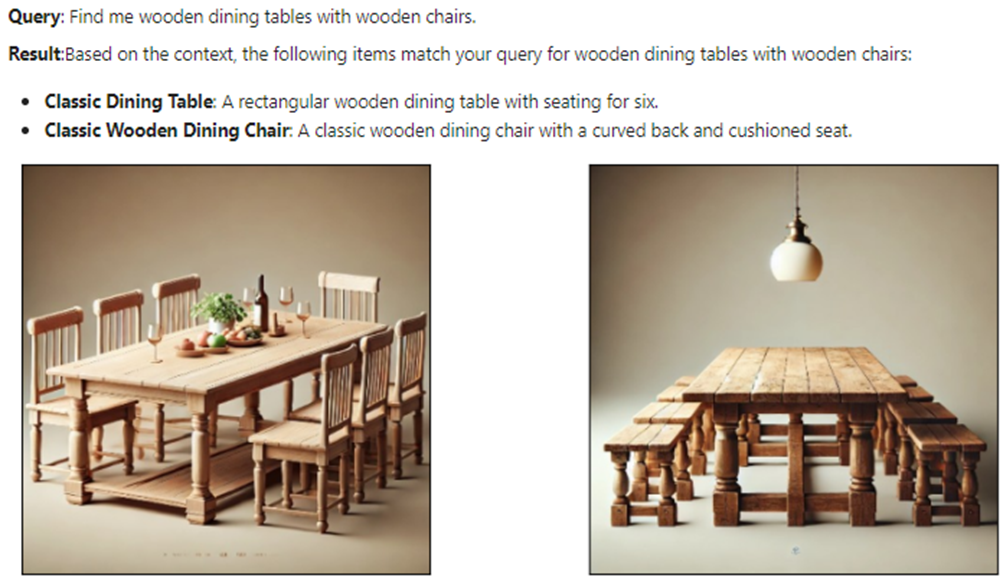
Let’s test the retriever for the query “Find me a chair with metal stands”. A helper function display_images plots the retrieved images.
###test retriever
from llama_index.core.response.notebook_utils import display_source_node
from llama_index.core.schema import ImageNode
import matplotlib.pyplot as plt
from PIL import Image
def display_images(file_list, grid_rows=2, grid_cols=3, limit=9):
"""
Display images from a list of file paths in a grid.
Parameters:
- file_list: List of image file paths.
- grid_rows: Number of rows in the grid.
- grid_cols: Number of columns in the grid.
- limit: Maximum number of images to display.
"""
plt.figure(figsize=(16, 9))
count = 0
for idx, file_path in enumerate(file_list):
if os.path.isfile(file_path) and count < limit:
img = Image.open(file_path)
plt.subplot(grid_rows, grid_cols, count + 1)
plt.imshow(img)
plt.axis('off')
count += 1
plt.tight_layout()
plt.show()
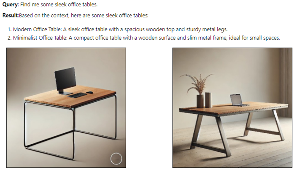
query = "Find me a chair with metal stands"
retrieval_results = retriever_engine.retrieve(query)
retrieved_image = []
for res_node in retrieval_results:
if isinstance(res_node.node, ImageNode):
retrieved_image.append(res_node.node.metadata["file_path"])
else:
display_source_node(res_node, source_length=200)
display_images(retrieved_image)
The text node and the images retrieved by the retriever are shown below.
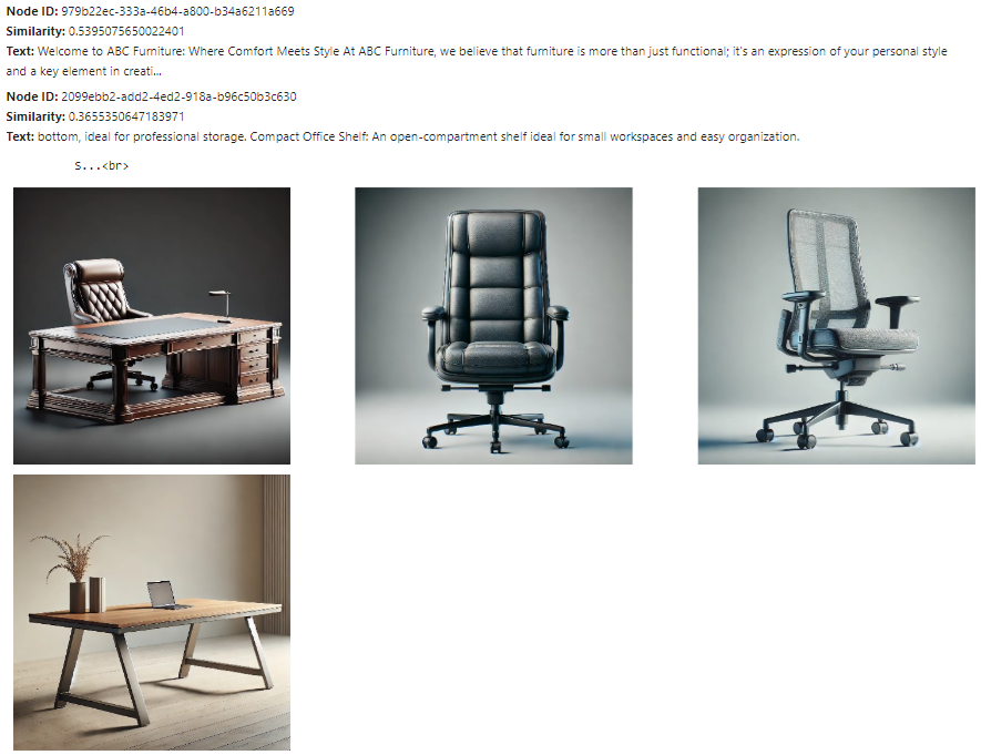
The text nodes and images retrieved here are close to the query embeddings, but not all may be relevant. The next step is to send these text nodes and images to a multimodal LLM to refine the selection and generate the final response. The prompt template qa_tmpl_str guides the LLM’s behavior in this selection and response generation process.
import logging
from llama_index.core.schema import NodeWithScore, ImageNode, MetadataMode

# Define the template with explicit instructions
qa_tmpl_str = (
    "Context information is below.n"
    "---------------------n"
    "{context_str}n"
    "---------------------n"
    "Using the provided context and images (not prior knowledge), "
    "answer the query. Include only the image paths of images that directly relate to the answer.n"
    "Your response should be formatted as follows:n"
    "Result: [Provide answer based on context]n"
    "Relevant Image Paths: array of image paths of relevant images only separated by comman"
    "Query: {query_str}n"
    "Answer: "
)

qa_tmpl = PromptTemplate(qa_tmpl_str)
# Initialize multimodal LLM
multimodal_llm = OpenAIMultiModal(model="gpt-4o", temperature=0.0, max_tokens=1024)
# Setup the query engine with retriever and prompt template
query_engine = index.as_query_engine(
    llm=multimodal_llm,
    text_qa_template=qa_tmpl,
    retreiver=retriever_engine
)
The following code creates the context string ctx_str for the prompt template qa_tmpl_str by preparing the image nodes with valid paths and metadata. It also embeds the query string with the prompt template. The prompt template, along with the embedded context, is then sent to the LLM to generate the final response.
# Extract the underlying nodes
nodes = [node.node for node in retrieval_results]

# Create ImageNode instances with valid paths and metadata
image_nodes = []
for n in nodes:
    if "file_path" in n.metadata and n.metadata["file_path"].lower().endswith(('.png', '.jpg')):
        # Add the ImageNode with only path and mimetype as expected by LLM
        image_node = ImageNode(
            image_path=n.metadata["file_path"],
            image_mimetype="image/jpeg" if n.metadata["file_path"].lower().endswith('.jpg') else "image/png"
        )
        image_nodes.append(NodeWithScore(node=image_node))
        logging.info(f"ImageNode created for path: {n.metadata['file_path']}")

logging.info(f"Total ImageNodes prepared for LLM: {len(image_nodes)}")

# Create the context string for the prompt
ctx_str = "nn".join(
    [n.get_content(metadata_mode=MetadataMode.LLM).strip() for n in nodes]
)

# Format the prompt
fmt_prompt = qa_tmpl.format(context_str=ctx_str, query_str=query)

# Use the multimodal LLM to generate a response
llm_response = multimodal_llm.complete(
    prompt=fmt_prompt,
    image_documents=[image_node.node for image_node in image_nodes],  # Pass only ImageNodes with paths
    max_tokens=300
)

# Convert response to text and process it
response_text = llm_response.text  # Extract the actual text content from the LLM response

# Extract the image paths after "Relevant Image Paths:"
image_paths = re.findall(r'Relevant Image Paths:s*(.*)', response_text)
if image_paths:
    # Split the paths by comma if multiple paths are present and strip any extra whitespace
    image_paths = [path.strip() for path in image_paths[0].split(",")]

# Filter out the "Relevant Image Paths" part from the displayed response
filtered_response = re.sub(r'Relevant Image Paths:.*', '', response_text).strip()

display(Markdown(f"**Query**: {query}"))

# Print the filtered response without image paths
display(Markdown(f"{filtered_response}"))

if image_paths!=['']:
    # Plot images using the paths collected in the image_paths array
    display_images(image_paths)
The final (filtered) response generated by the LLM for the above query is shown below.

This shows that the embedding model successfully connects the text embeddings with image embeddings and retrieves relevant results which are then further refined by the LLM.
The results of a few more test queries are shown below.

Now let’s test the multimodal embedding model for an image-to-image task. We use a different product image (not in the catalog) and use the retriever to bring the matching product images. The following code retrieves the matching product images with a modified helper function display_images.
import matplotlib.pyplot as plt
from PIL import Image
import os

def display_images(input_image_path, matched_image_paths):
    """
    Plot the input image alongside matching images with appropriate labels.
    """
    # Total images to show (input + first match)
    total_images = 1 + len(matched_image_paths)

    # Define the figure size
    plt.figure(figsize=(7, 7))

    # Display the input image
    plt.subplot(1, total_images, 1)
    if os.path.isfile(input_image_path):
        input_image = Image.open(input_image_path)
        plt.imshow(input_image)
        plt.title("Given Image")
        plt.axis("off")

    # Display matching images
    for idx, img_path in enumerate(matched_image_paths):
        if os.path.isfile(img_path):
            matched_image = Image.open(img_path)
            plt.subplot(1, total_images, idx + 2)
            plt.imshow(matched_image)
            plt.title("Match Found")
            plt.axis("off")

    plt.tight_layout()
    plt.show()

# Sample usage with specified paths
input_image_path = 'C:/Users/h02317/Downloads/trial2.png'

retrieval_results = retriever_engine.image_to_image_retrieve(input_image_path)
retrieved_images = []
for res in retrieval_results:
    retrieved_images.append(res.node.metadata["file_path"])

# Call the function to display images side-by-side
display_images(input_image_path, retrieved_images[:2])
Some results of the input and output (matching) images are shown below.
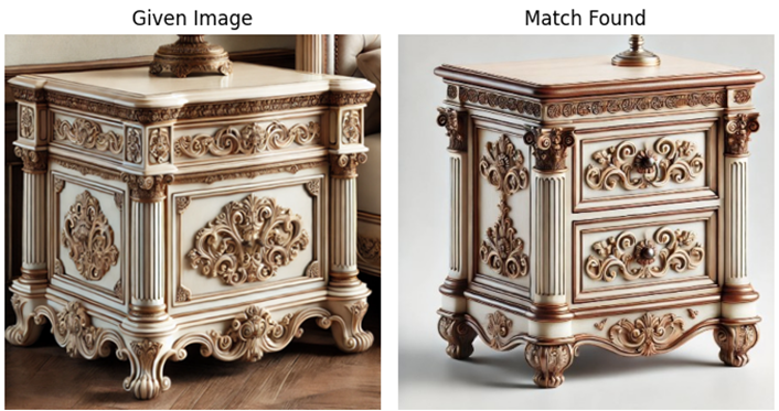
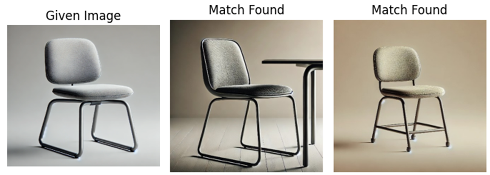
These results show that this multimodal embedding model offers impressive performance across text-to-text, text-to-image, and image-to-image tasks. This model can be further explored for multimodal RAGs with large documents to enhance retrieval experience with diverse data types.
In addition, multimodal embedding models hold good potential in various business applications, including personalized recommendations, content moderation, cross-modal search engines, and customer service automation. These models can enable companies to develop richer user experiences and more efficient knowledge retrieval systems.
If you like the article, please clap the article and follow me on Medium and/or LinkedIn
For the full code reference, please take a look at my repo:
Multimodal AI Search for Business Applications was originally published in Towards Data Science on Medium, where people are continuing the conversation by highlighting and responding to this story.
Originally appeared here:
Multimodal AI Search for Business Applications
Go Here to Read this Fast! Multimodal AI Search for Business Applications
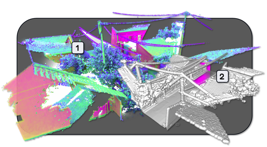
Learn how to generate 3D meshes from point cloud data with Python. This tutorial culminates in a 3D Modelling app with the Marching Cubes…
Originally appeared here:
Transform Point Clouds into 3D Meshes: A Python Guide
Go Here to Read this Fast! Transform Point Clouds into 3D Meshes: A Python Guide

Who said that the longer tails are not important? Let’s give them a proper way to stand out
Originally appeared here:
Awesome Plotly with Code Series (Part 3): Highlighting Bars in the Long Tails
OpenAI founder Sam Altman has made ambitious calculations, suggesting a potential investment scale of $7 trillion in GPUs for an AI future. This number, rejected by industry leaders like Nvidia’s founder Jensen Huang, implies a monumental acquisition of GPUs, requiring enormous energy, almost on a galactic scale. To put this in perspective, Nvidia’s current market worth is around $3 trillion, below half of Altman’s proposed investment. When compared to the GDPs of the United States (approximately $26.8 trillion) and China (around $17.8 trillion), this $7 trillion investment is still indeed staggering.
Despite this, the AI era is still in its infancy, and achieving such a scale might necessitate even more advanced computational structures. This brings us to a critical underlying question: how much energy will be needed to power computational units and data centers?
Let’s take a look at some simple and direct numbers from three perspectives,
1. Energy consumption per computational unit
2. Energy costs of training/operating modern models
3. Energy supply and demand
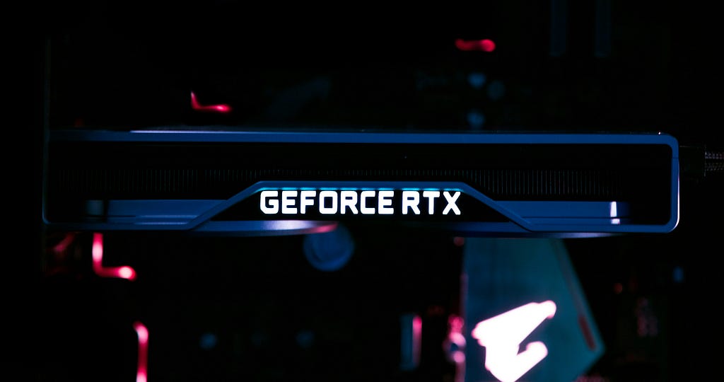
From a user perspective, some video game enthusiasts have built their own PCs equipped with high-performance GPUs like the NVIDIA GeForce RTX 4090. Interestingly, this GPU is also capable of handling small-scale deep-learning tasks. The RTX 4090 requires a power supply of 450 W, with a recommended total power supply of 850 W (in most cases you don’t need that and will not run under full load). If your task runs continuously for a week, that translates to 0.85 kW × 24 hours × 7 days = 142.8 kWh per week. In California, PG&E charges as high as 50 cents per kWh for residential customers, meaning you would spend around $70 per week on electricity. Additionally, you’ll need a CPU and other components to work alongside your GPU, which will further increase the electricity consumption. This means the overall electricity cost can be even higher.
Now, your AI business is going to accelerate. According to the manufacturer, an H100 Tensor Core GPU has a maximum thermal design power (TDP) of around 700 Watts, depending on the specific version. This is the energy required to cool the GPU under a full working load. A reliable power supply unit for this high-performance deep-learning tool is typically around 1600W. If you use the NVIDIA DGX platform for your deep-learning tasks, a single DGX H100 system, equipped with 8 H100 GPUs, consumes approximately 10.2 kW. For even greater performance, an NVIDIA DGX SuperPOD can include anywhere from 24 to 128 NVIDIA DGX nodes. With 64 nodes, the system could conservatively consume about 652.8 kW. While your startup might aspire to purchase this millions-dollar equipment, the costs for both the cluster and the necessary facilities would be substantial. In most cases, it makes more sense to rent GPU clusters from cloud computation providers. Focusing on energy costs, commercial and industrial users typically benefit from lower electricity rates. If your average cost is around 20 cents per kWh, operating 64 DGX nodes at 652.8 kW for 24 hours a day, 7 days a week would result in 109.7 MWh per week. This could cost you approximately $21,934 per week.
According to rough estimations, a typical family in California would spend around 150 kWh per week on electricity. Interestingly, this is roughly the same cost you’d incur if you were to run a model training task at home using a high-performance GPU like the RTX 4090.
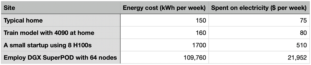
From this table, we may observe that operating a SuperPOD with 64 nodes could consume as much energy in a week as a small community.
Now, let’s dive into some numbers related to modern AI models. OpenAI has never disclosed the exact number of GPUs used to train ChatGPT, but a rough estimate suggests it could involve thousands of GPUs running continuously for several weeks to months, depending on the release date of each ChatGPT model. The energy consumption for such a task would easily be on the megawatt scale, leading to costs in the thousands scale of MWh.
Recently, Meta released LLaMA 3.1, described as their “most capable model to date.” According to Meta, this is their largest model yet, trained on over 16,000 H100 GPUs — the first LLaMA model trained at this scale.
Let’s break down the numbers: LLaMA 2 was released in July 2023, so it’s reasonable to assume that LLaMA 3 took at least a year to train. While it’s unlikely that all GPUs were running 24/7, we can estimate energy consumption with a 50% utilization rate:
1.6 kW × 16,000 GPUs × 24 hours/day × 365 days/year × 50% ≈ 112,128 MWh
At an estimated cost of $0.20 per kWh, this translates to around $22.4 million in energy costs. This figure only accounts for the GPUs, excluding additional energy consumption related to data storage, networking, and other infrastructure.
Training modern large language models (LLMs) requires power consumption on a megawatt scale and represents a million-dollar investment. This is why modern AI development often excludes smaller players.
Running AI models also incurs significant energy costs, as each inquiry and response requires computational power. Although the energy cost per interaction is small compared to training the model, the cumulative impact can be substantial, especially if your AI business achieves large-scale success with billions of users interacting with your advanced LLM daily. Many insightful articles discuss this issue, including comparisons of energy costs among companies operating ChatBots. The conclusion is that, since each query could cost from 0.002 to 0.004 kWh, currently, popular companies would spend hundreds to thousands of MWh per year. And this number is still increasing.

Imagine for a moment that one billion people use a ChatBot frequently, averaging around 100 queries per day. The energy cost for this usage can be estimated as follows:
0.002 kWh × 100 queries/day × 1e9 people × 365 days/year ≈ 7.3e7 MWh/year
This would require an 8000 MW power supply and could result in an energy cost of approximately $14.6 billion annually, assuming an electricity rate of $0.20 per kWh.

The largest power plant in the U.S. is the Grand Coulee Dam in Washington State, with a capacity of 6,809 MW. The largest solar farm in the U.S. is Solar Star in California, which has a capacity of 579 MW. In this context, no single power plant is capable of supplying all the electricity required for a large-scale AI service. This becomes evident when considering the annual electricity generation statistics provided by EIA (Energy Information Administration),

The 73 billion kWh calculated above would account for approximately 1.8% of the total electricity generated annually in the US. However, it’s reasonable to believe that this figure could be much higher. According to some media reports, when considering all energy consumption related to AI and data processing, the impact could be around 4% of the total U.S. electricity generation.
However, this is the current energy usage.
Today, Chatbots primarily generate text-based responses, but they are increasingly capable of producing two-dimensional images, “three-dimensional” videos, and other forms of media. The next generation of AI will extend far beyond simple Chatbots, which may provide high-resolution images for spherical screens (e.g. for Las Vegas Sphere), 3D modeling, and interactive robots capable of performing complex tasks and executing deep logistical. As a result, the energy demands for both model training and deployment are expected to increase dramatically, far exceeding current levels. Whether our existing power infrastructure can support such advancements remains an open question.
On the sustainability front, the carbon emissions from industries with high energy demands are significant. One approach to mitigating this impact involves using renewable energy sources to power energy-intensive facilities, such as data centers and computational hubs. A notable example is the collaboration between Fervo Energy and Google, where geothermal power is being used to supply energy to a data center. However, the scale of these initiatives remains relatively small compared to the overall energy needs anticipated in the upcoming AI era. There is still much work to be done to address the challenges of sustainability in this context.

Please correct any numbers if you find them unreasonable.
Massive Energy for Massive GPU Empowering AI was originally published in Towards Data Science on Medium, where people are continuing the conversation by highlighting and responding to this story.
Originally appeared here:
Massive Energy for Massive GPU Empowering AI
Go Here to Read this Fast! Massive Energy for Massive GPU Empowering AI


Exploring the limits of artificial intelligence: why mastering patterns may not equal genuine reasoning
Originally appeared here:
The Savant Syndrome: Is Pattern Recognition Equivalent to Intelligence?
Go Here to Read this Fast! The Savant Syndrome: Is Pattern Recognition Equivalent to Intelligence?


When I read the recent article in VentureBeat about how Glean just secured over $260 million in its latest funding round, I had two immediate gut feelings. First, it was satisfying to see this very public example of graph RAG living up to its potential as a powerful, valuable technology that connects people with knowledge more efficiently than ever. Second, it felt surprising but validating to read:
One of the world’s largest ride-sharing companies experienced its benefits firsthand. After dedicating an entire team of engineers to develop a similar in-house solution, they ultimately decided to transition to Glean’s platform.
“Within a month, they were seeing twice the usage on the Glean platform because the results were there,” says Matt Kixmoeller, CMO at Glean.
Although I was surprised to read about the failure in a news article, struggling to bring graph RAG into production is what I would expect, based on my experience as well as the experiences of coworkers and customers. I’m not saying that I expect large tech companies to fail at building their own graph RAG system. I merely expect that most folks will struggle to build out and productionize graph RAG — even if they already have a very successful proof-of-concept.
I wrote a high-level reaction to the VentureBeat article in The New Stack, and in this article, I’d like to dive deeper into why graph RAG can be so hard to get right. First, I’ll note how easy it has become, using the latest tools, to get started with graph RAG. Then, I’ll dig into some of the specific challenges of graph RAG that can make it so difficult to bring from R&D into production. Finally, I’ll share some tips on how to maximize your chances of success with graph RAG.
So if a big ride-sharing company couldn’t build their own platform effectively, then why would I say that it’s easy to implement graph RAG yourself?

Well, first of all, technologies supporting RAG and graph RAG have come a long way in the past year. Twelve months ago, most enterprises hadn’t even heard of retrieval-augmented generation. Now, not only is RAG support a key feature of the best AI-building tools like LangChain, but just about every major player in the AI space has a RAG tutorial, and there is even a Coursera course. There is no shortage of quick entry points for trying RAG.
Microsoft may not have been the first to do graph RAG, but they gave the concept a big push with a research blog post earlier this year, and they continue to work on related tech.
Here on Medium, there is also a nice conceptual introduction, with some technical details, from a gen AI engineer at Google. And, in Towards Data Science, there is a recent and very thorough how-to article on building a graph RAG system and testing on a dataset of scientific publications.
An established name in traditional graph databases and analytics, Neo4j, added vector capabilities to their flagship graph DB product in response to the recent gen AI revolution, and they have an excellent platform of tools for projects that require sophisticated graph analytics and deep graph algorithms in addition to standard graph RAG capabilities. They also have a Getting Started With Graph RAG guide.
On the other hand, you don’t even need a graph DB to do graph RAG. Many folks who are new to graph RAG believe that they need to deploy a specialized graph DB, but this is not necessary, and in fact may simply complicate your tech stack.
My employer, DataStax, also has a Guide to Graph RAG.
And, of course, the two most popular gen AI application composition frameworks, LangChain and LlamaIndex, each have their own graph RAG introductions. And there’s a DataCamp article that uses both.
With all of the tools and tutorials available, getting started with graph RAG is the easy part…
This is a very old story in data science: a new software methodology, technology, or tool solves some imposing problem in a research context, but industry struggles to build it into products that deliver value on a daily basis. It’s not just an issue of effort and proficiency in software development — even the biggest, best, and brightest teams might not be able to overcome the uncertainty, unpredictability, and uncontrollability of real-world data involved in solving real-world problems.

Uncertainty is an inherent part of building and using data-centric systems, which almost always have some elements of stochasticity, probability, or unbounded inputs. And, uncertainty can be even greater when inputs and outputs are unstructured, which is the case with natural language inputs and outputs of LLMs and other GenAI applications.
Folks who want to try graph RAG typically already have an existing RAG application that performs well for simple use cases, but fails on some of the more complex use cases and prompts requiring multiple pieces of information across a knowledge base, potentially in different documents, contexts, formats, or even data stores. When all of the information needed to answer a question is in the knowledge base, but the RAG system isn’t finding it, it seems like a failure. And from a user experience (UX) perspective, it is — the correct answer wasn’t given.
But that doesn’t necessarily mean there is a “problem” with the RAG system, which might be performing exactly as it was designed. If there isn’t a problem or a bug, but we still aren’t getting the responses we want, that must mean that we are expecting the RAG system to have a capability it simply doesn’t have.
Before we look at why specifically graph RAG is hard to bring into production, let’s take a look at the problem we’re trying to solve.
Because plain RAG systems (without knowledge graphs) retrieve documents based solely on vector search, only documents that are most semantically similar to the query can be retrieved. Documents that are not semantically similar at all — or not quite similar enough — are left out and are not generally made available to the LLM generating a response to the prompt at query time.
When the documents we need to answer a question in a prompt are not all semantically similar to the prompt, one or more of them is often missed by a RAG system. This can happen when answering the question requires a mix of generalized and specialized documents or terms, and when documents are detail-dense in the sense that some very important details for this specific prompt are buried in the middle of related details that aren’t as relevant to this prompt. See this article for an example of RAG missing documents because two related concepts (“Space Needle” and “Lower Queen Anne neighborhood” in this case) are not semantically similar, and see this article for an example of important details getting buried in detail-dense documents because vector embeddings are “lossy”.
When we see retrieval “failing” to find the right documents, it can be tempting to try to make vector search better or more tailored to our use case. But this would require fiddling with embeddings, and embeddings are complicated, messy, expensive to calculate, and even more expensive to fine-tune. Besides, that wouldn’t even be the best way to solve the problem.
For example, looking at the example linked above, would we really want to use an embedding algorithm that puts the text “Space Needle” and “Lower Queen Anne neighborhood” close together in semantic vector space? No, fine-tuning or finding an embedding algorithm that puts those two terms very close together in semantic space would likely have some unexpected and undesired side effects.
It is better not to try to force a semantic model to do a job that geographical or tourism information would be much better suited for. If I were a travel or tourism company who relied on knowing which neighborhood such landmarks are in, I would rather build a database that knows these things with certainty — a task that is much easier than making semantic vector search do the same task… without complete certainty.
So, the main issue here is that we have concepts and information that we know are related in some way, but not in semantic vector space. Some other (non-vector) source of information is telling us that there are connections among the wide variety of concepts we are working with. The task of building a graph RAG application is to effectively capture these connections between concepts into a knowledge graph, and to use the graph connections to retrieve more relevant documents for responding to a prompt.

To summarize the issue that we’re trying to tackle with graph RAG: there exists semi-structured, non-semantic information connecting many of the concepts that appear in my unstructured documents — and I would like to use this connection information to complement semantic vector search in order to retrieve documents that are best suited to answer prompts and questions within my use cases. We simply want to make retrieval better, and we want to use some external information or external logic to accomplish that, instead of relying solely on semantic vector search to connect prompts with documents,
Considering the above motivation — to use “external” information to make document connections that semantic search misses — there are some guiding principles that we can keep in mind while building and testing a graph RAG application:
Perhaps in a future article, we will dig into the nuances and potential impacts of following these principles, but for now, I’ll just note that this list is intended to jointly increase explainability, prevent over-complexity, and maximize efficiency of both building and using a graph RAG system.
Following these principles along with other core principles from software engineering and data science can increase your chances of successfully building a useful and powerful graph RAG app, but there are certainly pitfalls along the way, which we outline in the next section.

Anyone who has spent a lot of time building software around data, complex algorithms, statistics, and human users probably understands that there is a lot of uncertainty in building a system like graph RAG. Unexpected things can happen during data prep and loading, while building a knowledge graph, while querying and traversing the graph, during results compilation and prompt construction, and at virtually any other point in the workflow.
Above, we discussed how it’s easy to implement graph RAG to get preliminary results, but it can be hard to get good results, much less production-quality results. Next, we look at a few potential issues that you might encounter when building and testing a graph RAG application.
If the performance of your graph RAG system is about the same as with plain RAG, there can be any number of causes. Generally speaking, this seems to imply that the graph is not adding value to the system, but this could be caused by a low-quality knowledge graph, under-utilization of the graph, sub-optimal parameter settings, or many others. Or, there may not be a problem at all; vector search may be doing an excellent job of finding the right documents, and a graph simply isn’t needed.
What to look at:
If you’re seeing hallucinations with graph RAG that you didn’t see with plain RAG, I would suspect a bug or a bad parameter setting somewhere. If you are seeing a similar level of hallucinations, this sounds like a general problem beyond the graph aspects.
What to look at:
When your knowledge graph is “too big” or too dense, two main types of problems can occur. First, there could be issues with scaling, which I discuss below. Second, graph traversal could result in “too many” documents, which must then be re-ranked and filtered. If the re-ranking and filtering strategy doesn’t play well with the retrieval and graph traversal elements, you could end up filtering out important documents immediately after your graph just discovered them.
What to look at:
Per above, if the graph is “too big”, it might be filled with low-quality connections. And if the graph is “too small”, I would hope that the connections there are meaningful, which is good, but missing connections come in two main types. The first is caused by a bug in the graph construction process. The second is caused by graph construction that was not designed for it. Data in a different contexts or different formats may be processed differently by different graph-construction methods.
What to look at:
Do you feel like you can build a graph that is “too big” or one that is “too small”, but you can’t build something in the middle?
What to look at:
This is a classic Data Science problem: build really cool and cutting-edge methods, only to see development teams refuse or struggle to bring the code from your notebooks into the production stack. Sticking to the most popular, best supported, and largely open-source tools can make it easier to get to production, especially if your organization is already using those tools elsewhere.
What to look at:
The article Scaling Knowledge Graphs by Eliminating Edges in The New Stack shows one way to make graph RAG very scalable. Like above, the most popular, best supported, and largely open-source tools are usually the best path to painless scaling, but it’s not always easy.
What to look at:
The key to creating a successful graph RAG system lies in constructing a knowledge graph and traversal logic that complement semantic vector retrieval, not replacing or competing with it. The graph design should aim to connect the right nodes, knowledge, entities, and documents at the right time, enabling the assembly of the appropriate documents to produce the most helpful and actionable query response.

With respect to Glean, it should be noted that an internal document dataset is a perfect use case for graph RAG. A knowledge graph can connect people, projects, products, customers, meetings, locations, etc — and all of these are somewhat limited in number by the size of the organization and the work it does. Building and managing a graph of thousands of employees is much more tractable than, for example, trying to do the same with all of the people mentioned on Wikipedia or in a large database of financial or legal documents. So, possibly the first great decision that Glean made was to find a great use case for graph RAG to tackle.
One often understated aspect of graph RAG systems is the quality and reliability of the input data and the pipelines that get it there. This has more to do with data engineering and traditional software development than AI. In previous tech paradigms, connecting different data systems was challenging due to incompatible data types and access methods. Now, AI and LLMs enable the integration of disparate sources of unstructured data, allowing for the consolidation of data from various origins into a single RAG system. This integration capability enables LLMs to process and make sense of unstructured data from various sources, such as internal web pages, wikis, code repositories, databases, Google Docs, and chat logs. Simply connecting all of this information together and making it accessible from a single interface can be a big win.
Construction of graph RAG systems for any use case involves leveraging foundational components such as data stores for vectors and graphs, embeddings, and LLMs, enhanced by open-source orchestration tools like LangChain and LlamaIndex. These tools facilitate the development of robust, scalable, and efficient systems, promising a future where companies achieve substantial success by optimizing knowledge work through automation and streamlining.
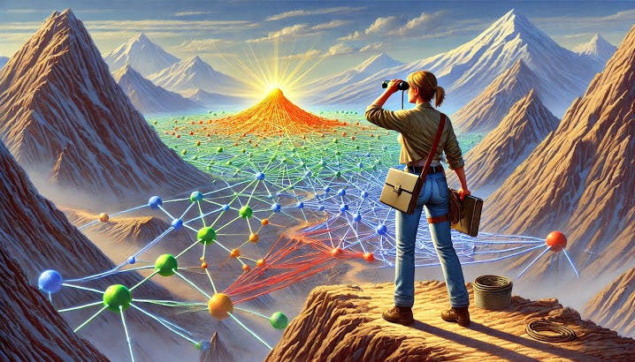
The public success of knowledge graphs and graph RAG systems, particularly by companies like Glean, showcases how effective these technologies are for internal use cases, creating value by making the organization more efficient. However, the broader application potential for external, enterprise and consumer-facing products remains largely untapped, presenting many opportunities for other companies to explore.
It is perhaps notable that we have been in what is called the “Information Age” for at least 30 years, and it is only in the past year or two that we have really started to put together the building blocks for connecting all of this information across sources, across ideas, across documents, and across concepts, so that our software systems can make the same types of reasoning, logic, and judgment that we as humans use as a daily part of our knowledge work. Some people are calling this the “Intelligence Age”.
While initially focusing on simple, straightforward decisions, AI’s trajectory is set towards managing more complex scenarios, dramatically improving efficiency in both time and cost. This exciting evolution positions many AI applications — including graph RAG — as pivotal in transforming how knowledge is interconnected and utilized in a wide variety of contexts.
To get started with graph RAG now, or to learn more, take a look at the DataStax guide to graph RAG.
by Brian Godsey, Ph.D. (LinkedIn) — mathematician, data scientist and engineer // AI and ML products at DataStax // Wrote the book Think Like a Data Scientist


The Quest for Production-Quality Graph RAG: Easy to Start, Hard to Finish was originally published in Towards Data Science on Medium, where people are continuing the conversation by highlighting and responding to this story.
Originally appeared here:
The Quest for Production-Quality Graph RAG: Easy to Start, Hard to Finish
Go Here to Read this Fast! The Quest for Production-Quality Graph RAG: Easy to Start, Hard to Finish