In this post, we demonstrate how to fine-tune Meta’s latest Llama 3.2 text generation models, Llama 3.2 1B and 3B, using Amazon SageMaker JumpStart for domain-specific applications. By using the pre-built solutions available in SageMaker JumpStart and the customizable Meta Llama 3.2 models, you can unlock the models’ enhanced reasoning, code generation, and instruction-following capabilities to tailor them for your unique use cases.
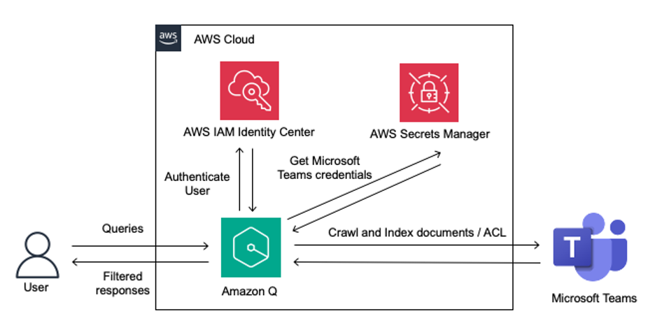
Microsoft Teams is an enterprise collaboration tool that allows you to build a unified workspace for real-time collaboration and communication, meetings, and file and application sharing. You can exchange and store valuable organizational knowledge within Microsoft Teams. Microsoft Teams data is often siloed across different teams, channels, and chats, making it difficult to get a […]
In the age of social media, analyzing conversation volumes has become crucial for understanding user behaviours, detecting trends, and, most importantly, identifying anomalies. Knowing when an anomaly is occurring can help management and marketing respond in crisis scenarios.
In this article, we’ll explore a residual-based approach for detecting anomalies in social media volume time series data, using a real-world example from Twitter. For such a task, I am going to use data from Numenta Anomaly Benchmark, which provides volume data from Twitter posts with a 5-minute frame window amongst its benchmarks.
We will analyze the data from two perspectives: as a first exercise we will detect anomalies using the full dataset, and then we will detect anomalies in a real-time scenario to check how responsive this method is.
Detecting anomalies with the full dataset
Analyzing a Sample Twitter Volume Dataset
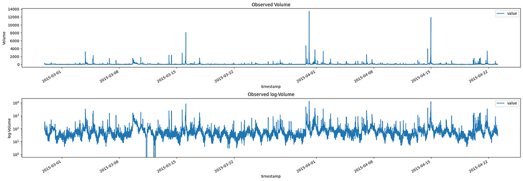
Let’s start by loading and visualizing a sample Twitter volume dataset for Apple:
Volume and log-Volume observed for AAPL Twitter volumes Image by Author
From this plot, we can see that there are several spikes (anomalies) in our data. These spikes in volumes are the ones we want to identify.
Looking at the second plot (log-scale) we can see that the Twitter volume data shows a clear daily cycle, with higher activity during the day and lower activity at night. This seasonal pattern is common in social media data, as it reflects the day-night activity of users. It also presents a weekly seasonality, but we will ignore it.
Removing Seasonal Trends
We want to make sure that this cycle does not interfere with our conclusions, thus we will remove it. To remove this seasonality, we’ll perform a seasonal decomposition.
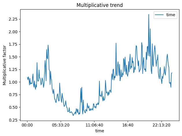
First, we’ll calculate the moving average (MA) of the volume, which will capture the trend. Then, we’ll compute the ratio of the observed volume to the MA, which gives us the multiplicative seasonal effect.
Multiplicative effect of time on volumes Image by Author
As expected, the seasonal trend follows a day/night cycle with its peak during the day hours and its saddle at nighttime.
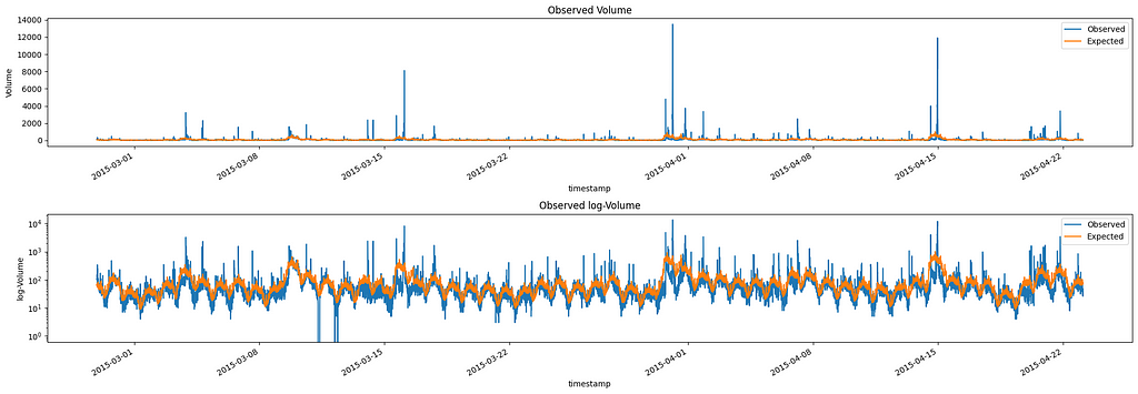
To further proceed with the decomposition we need to calculate the expected value of the volume given the multiplicative trend found before.
Volume and log-Volume observed and expected for AAPL Twitter volumes Image by Author
Analyzing Residuals and Detecting Anomalies
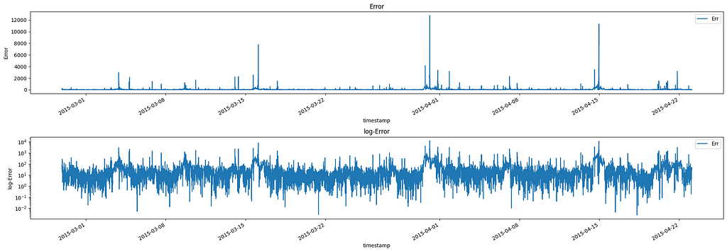
The final component of the decomposition is the error resulting from the subtraction between the expected value and the true value. We can consider this measure as the de-meaned volume accounting for seasonality:
Absolute Error and log-Error after seasonal decomposition of AAPL Twitter volumes Image by Author
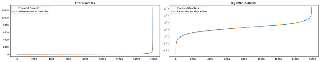
Interestingly, the residual distribution closely follows a Pareto distribution. This property allows us to use the Pareto distribution to set a threshold for detecting anomalies, as we can flag any residuals that fall above a certain percentile (e.g., 0.9995) as potential anomalies.
Absolute Error and log-Error quantiles Vs Pareto quantiles Image by Author
Now, I have to do a big disclaimer: this property I am talking about is not “True” per se. In my experience in social listening, I’ve observed that holds true with most social data. Except for some right skewness in a dataset with many anomalies.
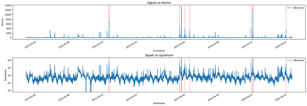
In this specific case, we have well over 15k observations, hence we will set the p-value at 0.9995. Given this threshold, roughly 5 anomalies for every 10.000 observations will be detected (assuming a perfect Pareto distribution).
Therefore, if we check which observation in our data has an error whose p-value is higher than 0.9995, we get the following signals:
Signals anomalies of AAPL Twitter volumes Image by Author
From this graph, we see that the observations with the highest volumes are highlighted as anomalies. Of course, if we desire more or fewer signals, we can adjust the selected p-value, keeping in mind that, as it decreases, it will increase the number of signals.
Real-Time Anomaly Detection
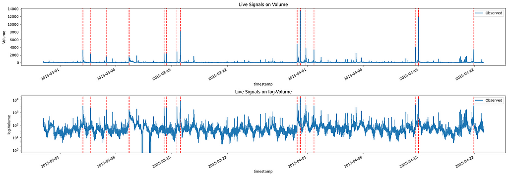
Now let’s switch to a real-time scenario. In this case, we will run the same algorithm for every new observation and check both which signals are returned and how quickly the signals are returned after the observation takes place:
Live Signals of AAPL Twitter volumes Image by Author
We can clearly see that this time, we have more signals. This is justified as the Pareto curve we fit changes as the data at our disposal changes. The first three signals can be considered anomalies if we check the data up to “2015–03–08” but these are less important if we consider the entire dataset.
By construction, the code provided returns with a signal limiting itself to the previous 24 hours. However, as we can see below, most of the signals are returned as soon as the new observation is considered, with a few exceptions already bolded:
New signal at datetime 2015-03-03 21:02:53, relative to timestamp 2015-03-03 21:02:53
New signal at datetime 2015-03-03 21:07:53, relative to timestamp 2015-03-03 21:07:53
New signal at datetime 2015-03-03 21:12:53, relative to timestamp 2015-03-03 21:12:53
New signal at datetime 2015-03-03 21:17:53, relative to timestamp 2015-03-03 21:17:53 **
New signal at datetime 2015-03-05 05:37:53, relative to timestamp 2015-03-04 20:07:53
New signal at datetime 2015-03-07 09:47:53, relative to timestamp 2015-03-06 19:42:53 **
New signal at datetime 2015-03-09 15:57:53, relative to timestamp 2015-03-09 15:57:53
New signal at datetime 2015-03-09 16:02:53, relative to timestamp 2015-03-09 16:02:53
New signal at datetime 2015-03-09 16:07:53, relative to timestamp 2015-03-09 16:07:53
New signal at datetime 2015-03-14 01:37:53, relative to timestamp 2015-03-14 01:37:53
New signal at datetime 2015-03-14 08:52:53, relative to timestamp 2015-03-14 08:52:53
New signal at datetime 2015-03-14 09:02:53, relative to timestamp 2015-03-14 09:02:53
New signal at datetime 2015-03-15 16:12:53, relative to timestamp 2015-03-15 16:12:53
New signal at datetime 2015-03-16 02:52:53, relative to timestamp 2015-03-16 02:52:53
New signal at datetime 2015-03-16 02:57:53, relative to timestamp 2015-03-16 02:57:53
New signal at datetime 2015-03-16 03:02:53, relative to timestamp 2015-03-16 03:02:53
New signal at datetime 2015-03-30 17:57:53, relative to timestamp 2015-03-30 17:57:53
New signal at datetime 2015-03-30 18:02:53, relative to timestamp 2015-03-30 18:02:53
New signal at datetime 2015-03-31 03:02:53, relative to timestamp 2015-03-31 03:02:53
New signal at datetime 2015-03-31 03:07:53, relative to timestamp 2015-03-31 03:07:53
New signal at datetime 2015-03-31 03:12:53, relative to timestamp 2015-03-31 03:12:53
New signal at datetime 2015-03-31 03:17:53, relative to timestamp 2015-03-31 03:17:53
New signal at datetime 2015-03-31 03:22:53, relative to timestamp 2015-03-31 03:22:53
New signal at datetime 2015-03-31 03:27:53, relative to timestamp 2015-03-31 03:27:53
New signal at datetime 2015-03-31 03:32:53, relative to timestamp 2015-03-31 03:32:53
New signal at datetime 2015-03-31 03:37:53, relative to timestamp 2015-03-31 03:37:53
New signal at datetime 2015-03-31 03:42:53, relative to timestamp 2015-03-31 03:42:53
New signal at datetime 2015-03-31 20:22:53, relative to timestamp 2015-03-31 20:22:53 **
New signal at datetime 2015-04-02 12:52:53, relative to timestamp 2015-04-01 20:42:53 **
New signal at datetime 2015-04-14 14:12:53, relative to timestamp 2015-04-14 14:12:53
New signal at datetime 2015-04-14 22:52:53, relative to timestamp 2015-04-14 22:52:53
New signal at datetime 2015-04-14 22:57:53, relative to timestamp 2015-04-14 22:57:53
New signal at datetime 2015-04-14 23:02:53, relative to timestamp 2015-04-14 23:02:53
New signal at datetime 2015-04-14 23:07:53, relative to timestamp 2015-04-14 23:07:53
New signal at datetime 2015-04-14 23:12:53, relative to timestamp 2015-04-14 23:12:53
New signal at datetime 2015-04-14 23:17:53, relative to timestamp 2015-04-14 23:17:53
New signal at datetime 2015-04-14 23:22:53, relative to timestamp 2015-04-14 23:22:53
New signal at datetime 2015-04-14 23:27:53, relative to timestamp 2015-04-14 23:27:53
New signal at datetime 2015-04-21 20:12:53, relative to timestamp 2015-04-21 20:12:53
As we can see, the algorithm is able to detect anomalies in real time, with most signals being raised as soon as the new observation is considered. This allows organizations to respond quickly to unexpected changes in social media conversation volumes.
Conclusions and Further Improvements
The residual-based approach presented in this article provides a responsive tool for detecting anomalies in social media volume time series. This method can help companies and marketers identify important events, trends, and potential crises as they happen.
While this algorithm is already effective, there are several points that can be further developed, such as:
Dependence on a fixed window for real-time detection, as for now depends on all previous data
Exploring different time granularities (e.g., hourly instead of 5-minute intervals)
Validating the Pareto distribution assumption using statistical tests
…
Please leave some claps if you enjoyed the article and feel free to comment, any suggestion and feedback is appreciated!
Part 2 of a hands-on guide to help you master MMM in pymc
User generated image
What is this series about?
Welcome to part 2 of my series on marketing mix modeling (MMM), a hands-on guide to help you master MMM. Throughout this series, we’ll cover key topics such as model training, validation, calibration and budget optimisation, all using the powerful pymc-marketing python package. Whether you’re new to MMM or looking to sharpen your skills, this series will equip you with practical tools and insights to improve your marketing strategies.
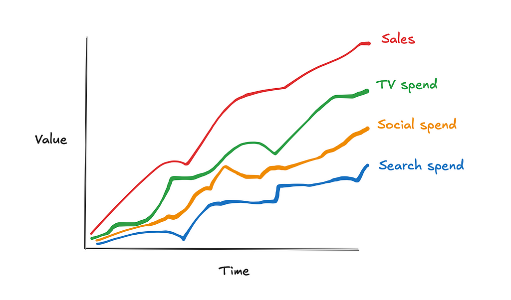
Marketing mix modelling (MMM) is a statistical technique used to estimate the impact of various marketing channels (such as TV, social media, paid search) on sales. The goal of MMM is to understand the return on investment (ROI) of each channel and optimise future marketing spend.
There are several reasons why we need to calibrate our models. Before we get into the python walkthrough let’s explore them a bit!
1. 1 Why is it important to calibrate marketing mix models?
Calibrating MMM is crucial because, while they provide valuable insights, they are often limited by several factors:
Multi-collinearity: This occurs when different marketing channels are highly correlated, making it difficult to distinguish their individual effects. For example, TV and social may run simultaneously, causing overlap in their impacts. Calibration helps untangle the effects of these channels by incorporating additional data or constraints.
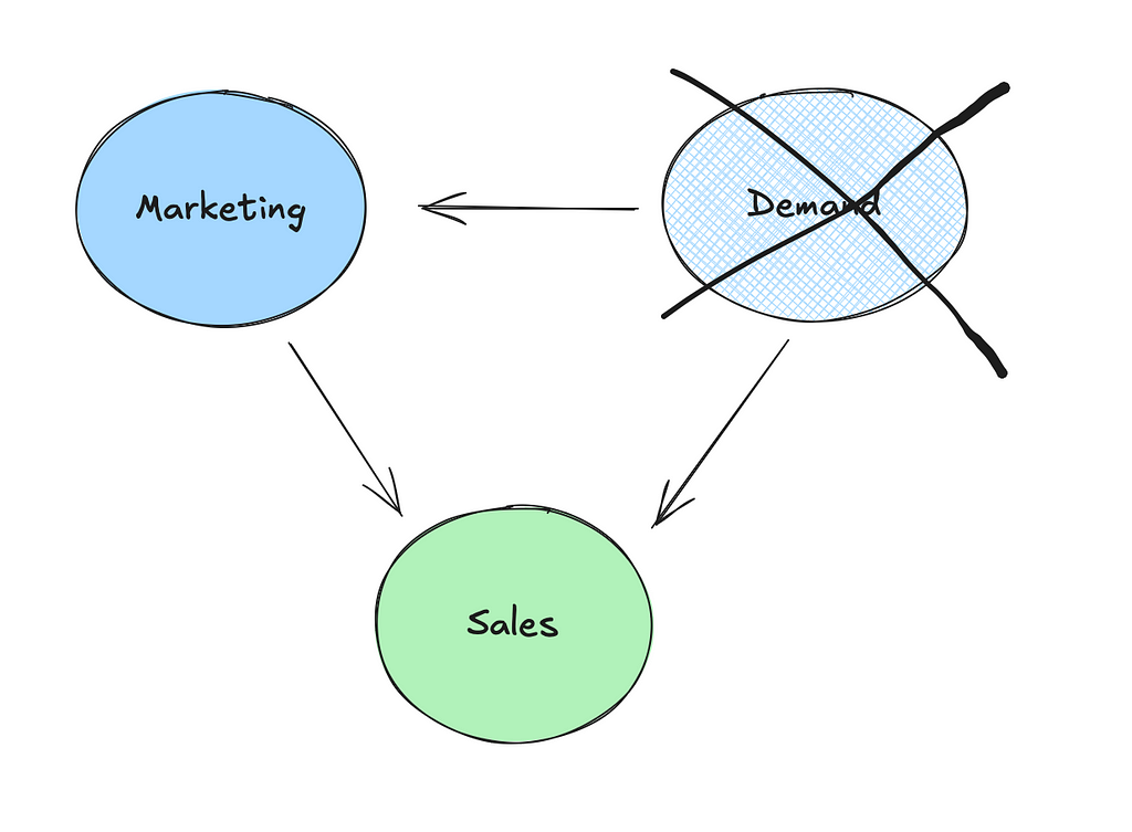
Unobserved confounders: MMM models rely on observed data, but they may miss important variables that also affect both marketing and sales, such as seasonality or changes in market demand. Calibration can help adjust for these unobserved confounders.
User generated image (excalidraw)
Re-targeting bias: Have you ever visited a website for a product and then found that all of your social media platforms are now suddenly “coincidently” showing you ads for that product? This isn’t a coincidence, it’s what we call retargeting and it can be effective. However, a number of prospects who get retargeted and then go on to purchase would have anyway!
Without proper calibration, these issues can lead to inaccurate estimates of marketing channel performance, resulting in poor decision-making on marketing spend and strategy.
1.2 How can we use Bayesian priors to calibrate our models?
In the last article we talked about how Bayesian priors represent our initial beliefs about the parameters in the model, such as the effect of TV spend on sales. We also covered how the default parameters in pymc-marketing were sensible choices but weakly informative. Supplying informative priors based on experiments can help calibrate our models and deal with the issues raised in the last section.
User generated image (excalidraw)
There are a couple of ways in which we can supply priors in pymc-marketing:
Change the default saturation_beta priors directly like in the example below using a truncated normal distribution to enforce positive values:
Use the add_lift_test_measurements method, which adds a new likelihood term to the model which helps calibrate the saturation curve (don’t worry, we will cover this in more detail in the python walkthrough):
What if you aren’t comfortable with Bayesian analysis? Your alternative is running a constrained regression using a package like cvxpy. Below is an example of how you can do that using upper and lower bounds for the coefficients of variables:
import cvxpy as cp
def train_model(X, y, reg_alpha, lower_bounds, upper_bounds): """ Trains a linear regression model with L2 regularization (ridge regression) and bounded constraints on coefficients.
Parameters: ----------- X : numpy.ndarray or similar Feature matrix where each row represents an observation and each column a feature. y : numpy.ndarray or similar Target vector for regression. reg_alpha : float Regularization strength for the ridge penalty term. Higher values enforce more penalty on large coefficients. lower_bounds : list of floats or None Lower bounds for each coefficient in the model. If a coefficient has no lower bound, specify as None. upper_bounds : list of floats or None Upper bounds for each coefficient in the model. If a coefficient has no upper bound, specify as None.
Returns: -------- numpy.ndarray Array of fitted coefficients for the regression model.
# Create constraints based on provided bounds constraints = ( [coef[i] >= lower_bounds[i] for i in range(X.shape[1]) if lower_bounds[i] is not None] + [coef[i] <= upper_bounds[i] for i in range(X.shape[1]) if upper_bounds[i] is not None] )
# Define and solve the problem problem = cp.Problem(objective, constraints) problem.solve()
# Print the optimization status print(problem.status)
return coef.value
1.3 What experiments can we run to inform our Bayesian priors?
Experiments can provide strong evidence to inform the priors used in MMM. Some common experiments include:
User generated image (excalidraw)
Conversion lift tests — These tests are often run on platforms like Facebook, YouTube, Snapchat, TikTok and DV360, where users are randomly split into a test and control group. The test group is exposed to the marketing campaign, while the control group is not. The difference in conversion rates between the two groups informs the actual lift attributable to the channel.
Geo-lift tests — In a geo-lift test, marketing efforts are turned off in certain geographic regions while continuing in others. By comparing the performance in test and control regions, you can measure the incremental impact of marketing in each region. The CausalPy python package has an easy to use implementation which is worth checking out:
Switch-back testing — This method involves quickly switching marketing campaigns on and off over short intervals to observe changes in consumer behavior. It’s most applicable to channels with an immediate impact, like paid search.
By using these experiments, you can gather strong empirical data to inform your Bayesian priors and further improve the accuracy and calibration of your Marketing Mix Model.
2.0 Python walkthrough
Now we understand why we need to calibrate our models, let’s calibrate our model from the first article! In this walkthrough we will cover:
Simulating data
Simulating experimental results
Pre-processing the experimental results
Calibrating the model
Validating the model
2.1 Simulating data
We are going to start by simulating the data used in the first article. If you want to understand more about the data-generating-process take a look at the first article where we did a detailed walkthrough:
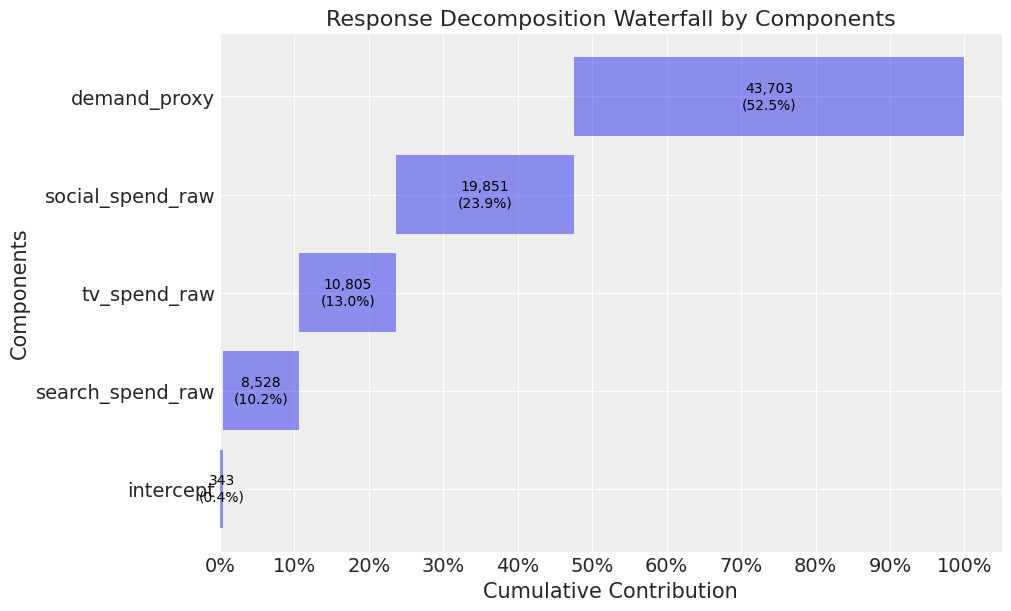
When we trained the model in the first article, the contribution of TV, social, and search were all overestimated. This appeared to be driven by the demand proxy not contributing as much as true demand. So let’s pick up where we left off and think about running an experiment to deal with this!
2.2 Simulating experimental results
To simulate some experimental results, we write a function which takes in the known parameters for a channel and outputs the true contribution for the channel. Remember, in reality we would not know these parameters, but this exercise will help us understand and test out the calibration method from pymc-marketing.
def exp_generator(start_date, periods, channel, adstock_alpha, saturation_lamda, beta, weekly_spend, max_abs_spend, freq="W"): """ Generate a time series of experiment results, incorporating adstock and saturation effects.
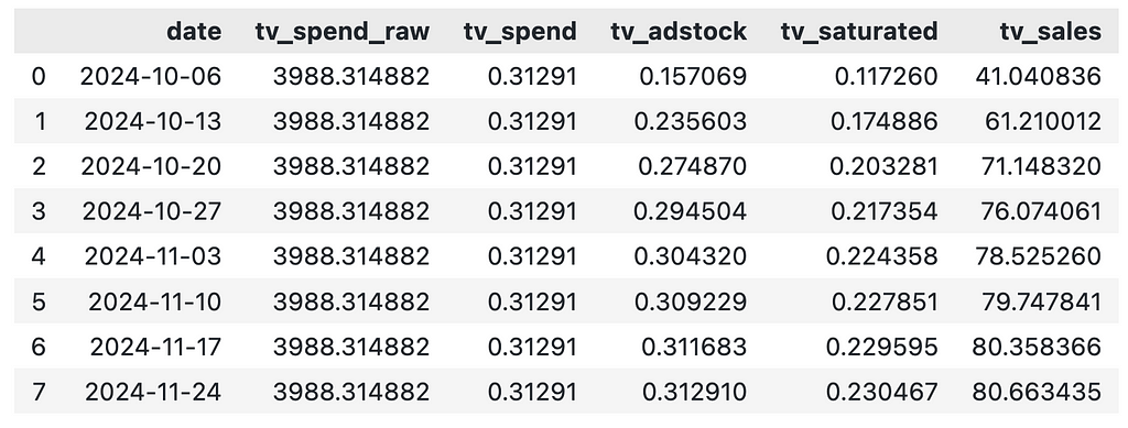
Parameters: ---------- start_date : str or datetime The start date for the time series. periods : int The number of time periods (e.g. weeks) to generate in the time series. channel : str The name of the marketing channel. adstock_alpha : float The adstock decay rate, between 0 and 1.. saturation_lamda : float The parameter for logistic saturation. beta : float The beta coefficient. weekly_spend : float The weekly raw spend amount for the channel. max_abs_spend : float The maximum absolute spend value for scaling the spend data, allowing the series to normalize between 0 and 1. freq : str, optional The frequency of the time series, default is 'W' for weekly. Follows pandas offset aliases Returns: ------- df_exp : pd.DataFrame A DataFrame containing the generated time series with the following columns: - date : The date for each time period in the series. - {channel}_spend_raw : The unscaled, raw weekly spend for the channel. - {channel}_spend : The scaled channel spend, normalized by `max_abs_spend`. - {channel}_adstock : The adstock-transformed spend, incorporating decay over time based on `adstock_alpha`. - {channel}_saturated : The adstock-transformed spend after applying logistic saturation based on `saturation_lamda`. - {channel}_sales : The final sales contribution calculated as the saturated spend times `beta`.
Even though we spend the same amount on TV each week, the contribution of TV varies each week. This is driven by the adstock effect and our best option here is to take the average weekly contribution.
weekly_sales = df_exp_tv["tv_sales"].mean()

weekly_sales
User generated image
2.3 Pre-processing the experimental results
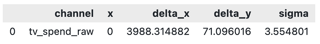
Now we have collected the experimental results, we need to pre-process them to get them into the required format to add to our model. We will need to supply the model a dataframe with 1 row per experiment in the following format:
channel: The channel that was tested
x: Pre-test channel spend
delta_x: Change made to x
delta_y: Inferred change in sales due to delta_x
sigma: Standard deviation of delta_y
We didn’t simulate experimental results with a measure of uncertainty, so to keep things simple we set sigma as 5% of lift.
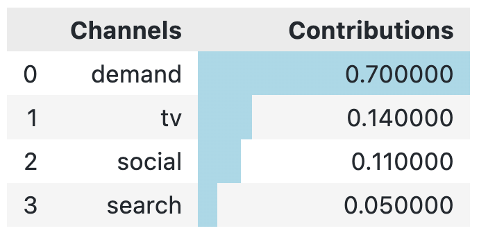
When we compare the true contributions to our new model, we see that the contribution of TV is now very close (and much closer than the model from our first article where the contribution was 24%!).
The contribution for search and social is still overestimated, but we could also run experiments here to deal with this.
Closing thoughts
Today we showed you how we can incorporate priors using experimental results. The pymc-marketing package makes things easy for the analyst running the model. However, don’t be fooled….There are still some major challenges on your road to a well calibrated model!
Logistical challenges in terms of constraints around how many geographic regions vs channels you have or struggling to get buy-in for experiments from the marketing team are just a couple of those challenges.
One thing worth considering is running one complete blackout on marketing and using the results as priors to inform demand/base sales. This helps with the logistical challenge and also improvs the power of your experiment (as the effect size increases).
I hope you enjoyed the second instalment! Follow me if you want to continue this path towards mastering MMM— In the next article we will start to think about dealing with mediators (specifically paid search brand) and budget optimisation.
Imitation Learning has recently gained increasing attention in the Machine Learning community, as it enables the transfer of expert knowledge to autonomous agents through observed behaviors. A first category of algorithm is Behavioral Cloning (BC), which aims to directly replicate expert demonstrations, treating the imitation process as a supervised learning task where the agent attempts to match the expert’s actions in given states. While straightforward and computationally efficient, BC often suffers from overfitting and poor generalization.
In contrast, Inverse Reinforcement Learning (IRL) targets the underlying intent of expert behavior by inferring a reward function that could explain the expert’s actions as optimal within the considered environment. Yet, an important caveat of IRL is the inherent ill-posed nature of the problem — i.e. that multiple (if not possibly an infinite number of) reward functions can make the expert trajectories as optimal. A widely adopted class of methods to tackle this ambiguity includes Maximum Entropy IRL algorithms, which introduce an entropy maximization term to encourage stochasticity and robustness in the inferred policy.
In this article, we choose a different route and introduce a novel iterative IRL algorithm that jointly learns both the reward function and the optimal policy from expert demonstrations alone. By iteratively synthesizing trajectories and guaranteeing their increasing quality, our approach departs from traditional IRL models to provide a fully tractable, interpretable and efficient solution.
The organization of the article is as follows: section 1 introduces some basic concepts in IRL. Section 2 gives an overview of recent advances in the IRL literature, which our model builds on. We derive a sufficient condition for the our model to converge in section 3. This theoretical result is general and can apply to a large class of algorithms. In section 4, we formally introduce the full model, before concluding on key differences with existing literature and further research directions in section 5.
1. Background definitions:
First let’s define a few concepts, starting with the general Inverse Reinforcement Learning problem (note: we assume the same notations as this article):
An Inverse Reinforcement Learning (IRL) problem is a 5-tuple (S, A, P, γ, τ*) such that:
S is the set of states the agent can be in
A is the set of actions the agent can take
P are transition probabilities
γ ∈ (0, 1] is a discount factor
τ* is the set of expert demonstrations, i.e. τ*ᵢ = (sᵢ, aᵢ) is a sequence of actions (sometimes called trajectory) taken by an expert agent
The goal of Inverse Reinforcement Learning is to infer the reward function R of the MDP (S, A, R, P, γ) solely from the expert trajectories. The expert is assumed to have full knowledge of this reward function and acts in a way that maximizes the reward of his actions.
We make the additional assumption of linearity of the reward function (common in IRL literature) i.e. that it is of the form:
where ϕ is a static feature map of the state-action space and w a weight vector. In practice, this feature map can be found via classical Machine Learning methods (e.g. VAE — see [6] for an example). The feature map can therefore be estimated separately, which reduces the IRL problem to inferring the weight vector w rather than the full reward function.
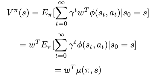
In this context, we finally derive the feature expectation μ, which will prove useful in the different methods presented. Starting from the value function of a given policy π:
We then use the linearity assumption of the reward function introduced above:
Likewise, μ can also be computed separately — usually via Monte Carlo.
2. Related work in RL and IRL literature
2.1 Apprenticeship Learning:
A seminal method to learn from expert demonstrations is Apprenticeship learning, first introduced in [1]. Unlike pure Inverse Reinforcement Learning, the objective here is to both to find the optimal reward vector as well as inferring the expert policy from the given demonstrations. We start with the following observation:
Mathematically this can be seen using the Cauchy-Schwarz inequality. This result is actually quite powerful, as it allows to focus on matching the feature expectations, which will guarantee the matching of the value functions — regardless of the reward weight vector.
In practice, Apprenticeship Learning uses an iterative algorithm based on the maximum margin principle to approximate μ(π*) — where π* is the (unknown) expert policy. To do so, we proceed as follows:
Start with a (potentially random) initial policy and compute its feature expectation, as well as the estimated feature expectation of the expert policy from the demonstrations (estimated via Monte Carlo)
For the given feature expectations, find the weight vector that maximizes the margin between μ(π*) and the other (μ(π)). In other words, we want the weight vector that would discriminate as much as possible between the expert policy and the trained ones
Once this weight vector w’ found, use classical Reinforcement Learning — with the reward function approximated with the feature map ϕ and w’ — to find the next trained policy
Repeat the previous 2 steps until the smallest margin between μ(π*) and the one for any given policy μ(π) is below a certain threshold — meaning that among all the trained policies, we have found one that matches the expert feature expectation up to a certain ϵ
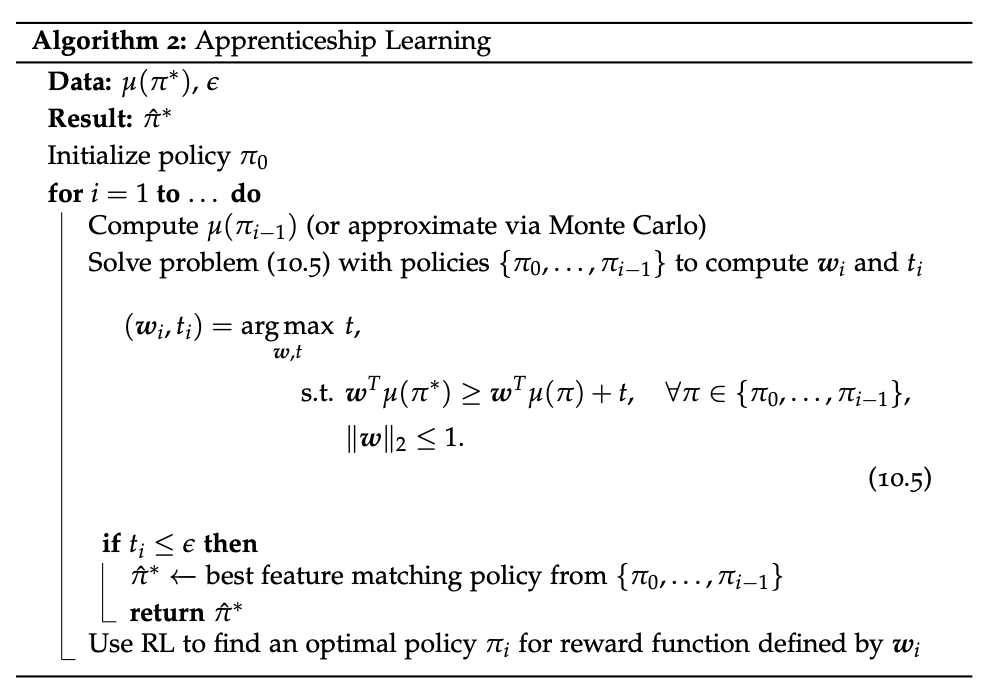
Written more formally:
Source: Principles of Robot Autonomy II, lecture 10 ([2])
2.2 IRL with ranked demonstrations:
The maximum margin principle in Apprenticeship Learning does not make any assumption on the relationship between the different trajectories: the algorithm stops as soon as any set of trajectories achieves a narrow enough margin. Yet, suboptimality of the demonstrations is a well-known caveat in Inverse Reinforcement Learning, and in particular the variance in demonstration quality. An additional information we can exploit is the ranking of the demonstrations — and consequently ranking of feature expectations.
More precisely, consider ranks {1, …, k} (from worst to best) and feature expectations μ₁, …, μₖ. Feature expectation μᵢ is computed from trajectories of rank i. We want our reward function to efficiently discriminate between demonstrations of different quality, i.e.:
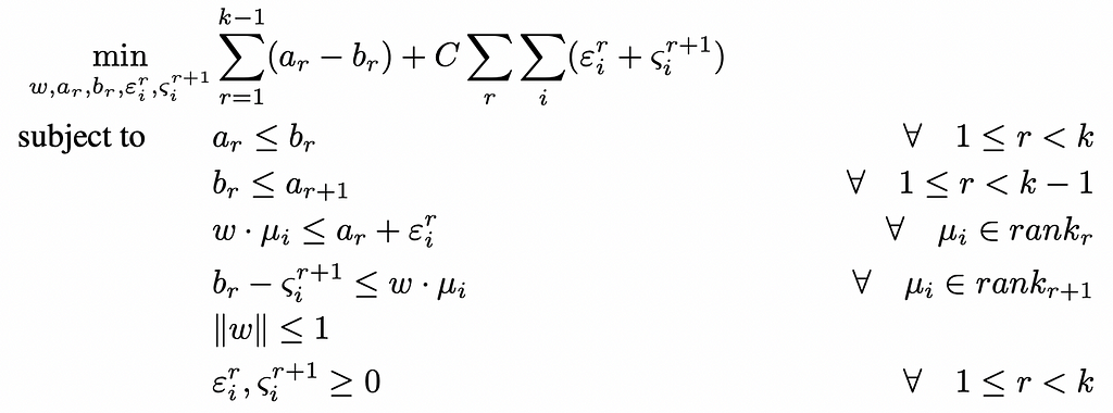
In this context, [5] presents a tractable formulation of this problem into a Quadratic Program (QP), using once again the maximum margin principle, i.e. maximizing the smallest margin between two different classes. Formally:
This is actually very similar to the optimization run by SVM models for multiclass classification. The all-in optimization model is the following — see [5] for details:
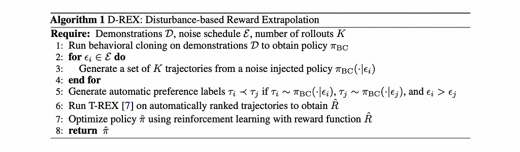
Presented in [4], the D-REX algorithm also uses this concept of IRL with ranked preferences but on generated demonstrations. The intuition is as follows:
Starting from the expert demonstrations, imitate them via Behavioral cloning, thus getting a baseline π₀
Generate ranked sets of demonstration with different degrees of performance by injecting different noise levels to π₀: in [4] authors prove that for two levels of noise ϵ and γ, such that ϵ > γ (i.e. ϵ is “noisier” than γ) we have with high probability that V[π(. | ϵ)] < V[π’. | γ)]- where π(. | x) is the policy resulting from injecting noise x in π₀.
Given this automated ranking provided, run an IRL from ranked demonstrations method (T-REX) based on approximating the reward function with a neural network trained with a pairwise loss — see [3] for more details
With the approximation of the reward function R’ gotten from the IRL step, run a classical RL method with R’ to get the final policy
More formally:
Source: [4]
Another important theoretical result presented in [4] is the effect of ranking on reward ambiguity: the paper manages to quantify the ambiguity reduction coming from added ranking constraint, which elegantly tackles the ill-posed nature of IRL.
2.4 Guided Reinforcement Learning:
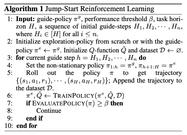
How can we leverage some expert demonstrations when fitting a Reinforcement Learning model? Rather than start exploring using an initial random policy, one could think of leveraging available demonstration information — as suboptimal as they might be — as a warm start and guide at least the beginning of the RL training. This idea is formalized in [8], and the intuition is:
For each training iteration, start with the expert policy / demonstrations (πᵍ) — to collect “good” samples and put the agent in “good” states
After a determined switch point, let the current trained policy (πᵉ) take over and explore states — the objective being that it explores states that have not been visited (enough) by the expert demonstrations, while relying on the expert choices for the visited ones
As it gets better, πᵉ should take over earlier
More formally:
Source: [8]
3. A sufficient condition for convergence:
Before deriving the full model, we establish the following result that will provide a useful bound guaranteeing improvement in an iterative algorithm — full proof is provided in the Appendix:
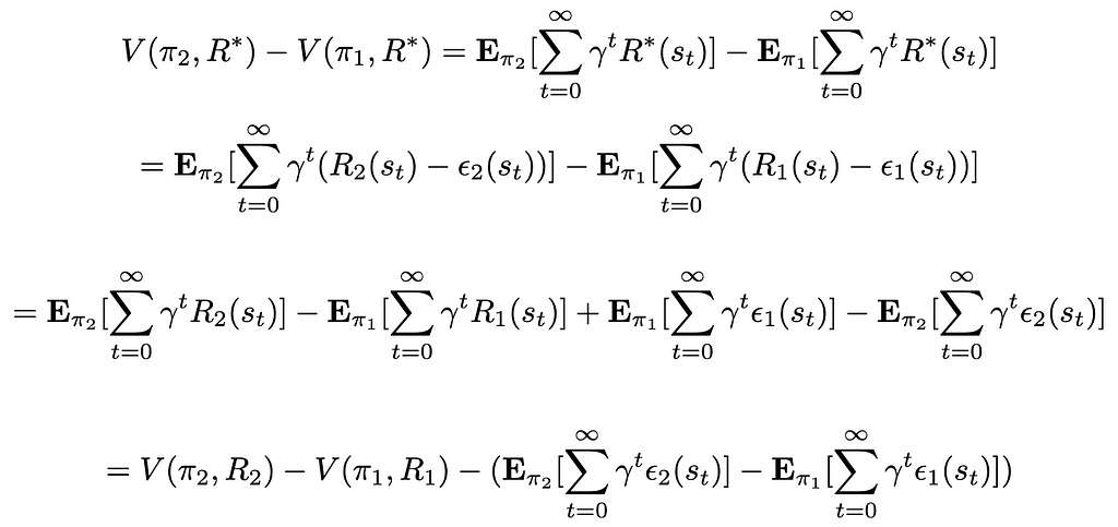
Theorem 1:Let (S, A, P, γ, π*) the Inverse Reinforcement Learning problem with unknown true reward function R*. For two policies π₁ and π₂ fitted using the candidate reward functions R₁ and R₂ of the form Rᵢ = R* + ϵᵢ with ϵᵢ some error function, we have the following sufficient condition to have π₂ improve upon π₁, i.e. V(π₂, R*) > V(π₁, R*):
Where TV(π₂, π₁) is the total variation distance between π₂ and π₁, interpreting the policies as probability measures.
This bound gives some intuitive insights, since if we want to guarantee improvement on a known policy with its reward function, the margin gets higher the more:
Different the two reward functions are
Different the two policies are
Imprecise the original reward function is
4. The full tractable model
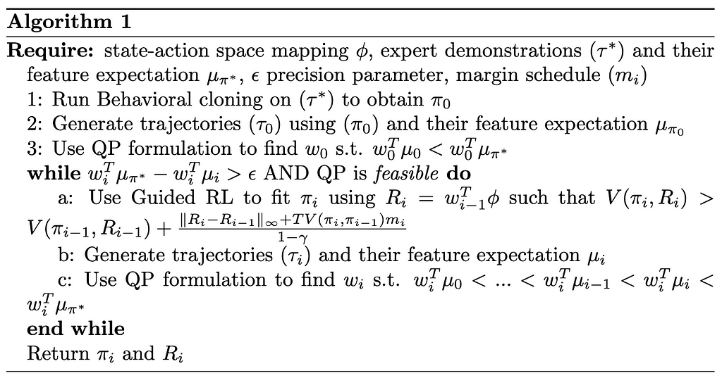
Building on the previously introduced models and Theorem 1, we can derive our new fully tractable model. The intuition is:
Initialization: start from the expert trajectories (τ*), estimate an initial policy π₀ (e.g. via Behavioral Cloning) and generate trajectories (τ₀) of an agent following π₀. Use these trajectories to estimate a reward weight vector w₀ (which gives R₀ = w₀ ϕ )such that V(π*, R₀) > V(π₀, R₀) through the Quadratic Program presented in section 2.2 — i.e. the ranking here being: {2 : τ*, 1: τ₀}
Iteration: infer a policy πᵢ using wᵢ-₁ (i.e. Rᵢ = wᵢ-₁ϕ) such that we have V(πᵢ, Rᵢ) > V(πᵢ-₁, Rᵢ-₁) with sufficient marginusing Guided RL. Note that here we do not necessarily want πᵢ to be optimal w.r.t. Rᵢ, we simply want something that outperforms the current policy by a certain margin as dictated by Theorem 1. The rationale behind this is that we do not want to overfit on the inaccuracies caused by the reward misspecification. See [7] for more details on the impact of this misspecification.
Likewise, generate samples τᵢ with policy πᵢ and use the tractable IRL model on the following updated ranking: {i : τ*, i-1: τᵢ, i-2: τᵢ-₁…}
Stopping condition: when V(τ*, wᵢ) — V(τᵢ, wᵢ) is below a certain threshold ϵ or if the Quadratic Program is infeasible
Formally:
This algorithm makes a few choices that we need to keep in mind:
An implicit assumption we make is that the reward functions are getting more precise through the iterations, i.e. the noise terms ϵᵢ are decreasing in norm and go to 0
Since the noise terms ϵᵢ are unknown, we replace them with a predetermined margin schedule (mᵢ)— following the above assumption we can make the schedule decreasing and going to 0
Why stop the iteration if the QP is infeasible: we know that the QP was feasible at the previous iteration, therefore the main constraint that made it infeasible was adding the new feature expectation μᵢ computed with trajectories using πᵢ. We interpret this infeasibility as the fact that we’re unable to get a margin significant enough to discriminate between μᵢ and μ*,which can mean that wᵢ-₁ and πᵢ are optimal solutions.
5. Conclusion and future work:
While synthesizing multiple models from RL and IRL literature, this new heuristic innovates in a number of ways:
Full tractability: not using a neural network for the IRL step is a choice, as it enhances tractability and interpretability. It also provides additional insights related to the feasibility of the QP which can allow to stop the algorithm earlier.
Efficiency and ease of use: although an iterative algorithm, each step of the iteration can be done very efficiently: the QP can be solved quickly using current solvers and the RL step requires only a limited number of iterations to satisfy the improvement condition presented in Theorem 1. It also offers additional flexibility with the ϵ coefficient, allowing the user to “pay” some suboptimality for faster convergence if needed.
Better use of all information available to minimize noise: the iterative nature of the algorithm limits the uncertainty propagation from IRL to RL as we always restart the fitting (offering a possibility to course-correct). The Guided RL step also allows to introduce a healthy bias towards the expert demonstrations.
We can also note that Theorem 1 is a general property and provides a bound that can be applied to a large class of algorithms.
Further research can naturally be done to extend this algorithm. First, a thorough implementation and benchmarking against other approaches can provide interesting insights. Another direction would be deepening the theoretical study of the convergence conditions of the model, especially the assumption of reduction of reward noise.
Appendix:
We prove Theorem 1 introduced earlier similarly to the proof of Theorem 1 in [4]. The target inequality for two given policies fitted at steps i and i-1 is: V(πᵢ, R*) > V(πᵢ-₁, R*). The objective is to derive a sufficient condition for this inequality to hold. We start with the following assumptions:
π₁ is the policy fitted at the previous iteration using the reward function R₁
The RL step uses a form of iterative algorithm (e.g. Value Iteration), which yields that at the current iteration π₂ is also known — even if it is only a candidate policy that could be improved if it does not fit the condition. The reward function it is (currently being) fitted on is R₂
The reward functions Rᵢ are of the form: Rᵢ = R* + ϵᵢ with ϵᵢ some error function
We thus have:
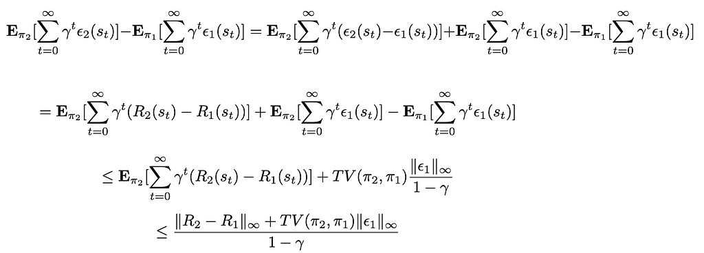
Following the assumptions mades, V(π₂, R₂) — V(π₁, R₁) is known at the time of the iteration. For the second part of the expression featuring ϵ₁ and ϵ₂ (which are unknown, as we only know ϵ₁ — ϵ₂ = R₁ — R₂) we derive an upper bound for its value:
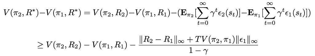
Where TV(π₁, π₂) is the total variance between π₁ and π₂, as we interpret the policies as probability measures. We reinject this upper bound in the first expression, giving:
Therefore, this gives the following condition to have the policy π₂ improve on π₁:
[8] I. Uchendu, T. Xiao, Y. Lu, B. Zhu, M. Yan, J. Simon, M. Bennice, Ch. Fu, C. Ma, J. Jiao, S. Levine, K. Hausman, Jump-Start Reinforcement Learning (2023), Proceedings of Machine Learning Research
I am often asked by people trying to break into data what skills they need to learn to get their first job in Data, and where they should learn them. This article is the distillation of the advice I have been giving aspiring data scientists, analysts, and engineers for the last 5 years.
This article is primarily geared towards self-taught data jockeys who are looking to land their first role in data. If you’re reading this article, odds are your first role will be as an analyst. Most of the entry level roles in data are analyst roles and I don’t regard data scientist or data engineering roles as entry level.
The four pillars are spreadsheets, SQL, a visualization tool, and a scripting language.
Different jobs will require a different blend of these skills, and you can build an entire career out of mastering just one of the pillars, but almost all roles in data require at least a cursory knowledge of the four subjects.
Excel is the alpha and omega of the data world. For 30 years the data community has been talking about the fabled “excel killer” and it hasn’t ever been found. You could have been part of a multi-team 6-month long effort to harmonize data from 7 databases, built them into the sexiest Tableau dashboard, and the first thing your stakeholders will ask you is how they can export it to excel.
Excel is vast and most users just scratch the surface of its functionality, but this is a list of skills that I would consider a minimum for landing an analyst role:
Basic interface navigation
Formulas
Conditionals (IF, IFS, COUNTIFS, SUMIFS, etc)
Spreadsheet hygiene (making sure your spreadsheets are logically laid out)
Joining data sets (V-lookup, X-lookup, index-match)
Charting/visualization
Pivot tables
Filtering and sorting data
Power Query
If you want to take it a step further, I also recommend aspiring analysts become familiar with Power Query (also called Get and Transform). I like power query for aspiring analysts because it is a good introduction to working with more formally structured data and working with proper tabular data.
One advantage of learning Power Query and Power Pivot is that they are extensively used in Power BI.
What about google sheets?
Google sheets is a solid spreadsheet alternative to Excel, but it is missing a lot of the advanced features. If you learn excel you can quickly adapt to google sheets, and you can learn many of the basic spreadsheet functions on google sheets, but I don’t think it’s an adequate substitute for excel at this point.
My observation is that Google sheets is commonly used in government, academia, and in early to middle stage startups.
VBA
If you’re trying to figure out how to do something in excel and the tutorial you stumble across suggests VBA, look for a different solution.
This is a tricky subject for aspiring analysts to learn because outside of a production environment it is hard to learn the nuances of working with databases beyond basic syntax. This is because most of the practice data sets are far too clean.
Early in one of my jobs I completely botched a SQL query request because I made the amateur mistake of joining two tables on the FINANCING_ID column instead of the FINANCING_ID_NEW column.
Most databases at organizations large enough to hire analysts are not planned or designed, but are rather organic accretions of data that build up over time, accrued via mergers and acquisitions and time constrained software engineers trying to solve a problem RIGHT NOW.
For many organizations, it can take months to onboard to their databases.
So my advice is aside from learning the basic syntax of one dialect of SQL, I wouldn’t spend too much time mastering SQL until you have a job where you get to write it every day.
These are the basic querying skills I suggest you learn:
Basic syntax
Anatomy of a SQL query
Aggregations
Multi-table joins
Dimensional modeling
CTEs and Subqueries
Which dialect should you learn?
It doesn’t really matter because they’re so similar and once you know one, the differences can all be resolved with google or Chat GPT. My suggestion is either Postgres or T-SQL.
While excel can be used to produce some visualizations, most organizations that hire analysts will produce dashboards with either Power BI or Tableau (I’ve worked with a few others but these are the dominant players).
Like SQL, I wouldn’t suggest indexing too heavily in visualization until after you have a job, learning the basics is important, but much of the advanced functionality is best learned in a production environment.
Power BI or Tableau?
I would suggest choosing one and focusing on it, rather then splitting your attention between the two.
If your primary experience in data is with Excel, Power BI will likely be more intuitive for you to work with. Once you learn to use one, you can easily adapt to learning another, and for most generalist analyst roles, hiring managers won’t care that much, as long as you know one of them.
I once interviewed for a role at a large enterprise to develop Tableau dashboards and I asked the hiring manager “if you hired me, what would you consider a successful hire after 6 months.”
His answer was “If you could edit a single dashboard after 6 months, I’ll consider it a success.”
Like SQL, a lot of the challenge of working with visualization tools is understanding the organization’s data.
What should you learn?
Making all of the standard charts
Data cleanup, and how data should be structured going into the tool of your choice
Finally we have scripting languages. As a caveat, my first few analyst roles didn’t require me to know a scripting language, but that was some time ago and reviewing application requirements, it appears that at least knowing a little is a requirement for entry level roles now.
R or Python?
If you already know R (learned it in a statistics class) then focus on R, otherwise learn Python. If you’re proficient in one, you can learn the syntax of the other in the time it takes you to onboard.
R also tends to be more common in organizations that have close relationships with academia. Biotech firms are more likely to use R because their researchers are more likely to have used it in grad school.
What should you learn?
Variables
Basic numeric manipulation
String manipulation
Conditionals (If/then)
Basic data structures (Lists, dictionaries, tuples, sets)
Loops
Defining and using functions
Pandas (the library, not the animal)
General advice
You don’t need to be an expert on these subjects, you need to be familiar with them.
For entry level analyst roles, focus most on excel.
Don’t overestimate your skill level. I once interviewed a candidate who described themselves as an “intermediate” Python user. The role didn’t call for Python, but since they said they could, I gave them a live coding exercise. I asked them to define a function to detect whether a given string input is a palindrome (a word spelled the same way forwards and backwards). They then admitted they didn’t know how to define a function. I politely ended the interview there.
For the most part, I don’t think certifications are particularly useful for securing entry level roles. They might make a difference at the margins (maybe you get an interview with a recruiter that you otherwise wouldn’t get), but I don’t think they’re worth the effort.
There is one exception to this: The South Asian job market.
I did use a handful of certifications as a heuristic when evaluating candidates.
Generally those certifications had a few things in common:
They were from major technology companies in data, like Snowflake, Microsoft, or Tableau.
They cost several hundred US dollars to obtain, representing a substantial investment for a typical South Asian employee (or their employer).
Free certificates
There are lots of free or very low cost certificates, like the Google Data certificates. In general I think they’re worth about as much as you pay for them. The learning content is solid, and they’re well put together curricula, but the certification itself won’t really help you stand out.
When I interview candidates, I really want them to succeed, I suspect most interviewers are the same.
So when you’re interviewing, keep it conversational.
I am mostly interested in seeing how you arrive at the right answer, not whether you get the answer. I prefer candidates to ask questions, test ideas, and ask for clarification. If you’re on the wrong track, I will ask questions to see if I can get you on the right track.
The following are mostly paid resources that I used when learning these skills. These are not referral links, I don’t get anything from you getting them.
Excel
Tom Hinkle is a dear friend, and I strongly recommend his courses on Udemy.
The IMDB’s actual database: This is a very clean dataset that will let you practice complex SQL queries across a dimensionally modeled database.
The Microsoft Contoso Database: This simulates a retail website’s database, and will give you good practice on aggregations, and answering business questions.
The Python Bible: Ziyad is one of the most engaging online instructors out there.
The Complete Pandas Bootcamp: Alexander Hagman is dry, but thorough. I still reference this course when I need refreshers on Pandas.
General
Anil was an early mentor of mine and has since started a digital analytics mentorship/educational platform. He taught me at a local college, but his work is stellar and he invests a lot in his students.
Do you think there are any foundational analytical skills I missed?
About the Author
Charles Mendelson is a senior software engineer at a Big 3 management consulting firm where he helps clients build AI prototypes and MVPs.
He started his tech career as a self-taught data analyst, before becoming a data engineer.
Solving the Classic Betting on the World Series Problem Using Hill Climbing
A simple example of hill climbing — and solving a problem that’s difficult to solve without optimization techniques
Betting on the World Series is an old, interesting, and challenging puzzle. It’s also a nice problem to demonstrate an optimization technique called hill climbing, which I’ll cover in this article.
Hill climbing is a well-established, and relatively straightforward optimization technique. There are many other examples online using it, but I thought this problem allowed for an interesting application of the technique and is worth looking at.
One place the puzzle can be seen in on a page hosted by UC Davis. To save you looking it up, I’ll repeat it here:
[E. Berlekamp] Betting on the World Series. You are a broker; your job is to accommodate your client’s wishes without placing any of your personal capital at risk. Your client wishes to place an even $1,000 bet on the outcome of the World Series, which is a baseball contest decided in favor of whichever of two teams first wins 4 games. That is, the client deposits his $1,000 with you in advance of the series. At the end of the series he must receive from you either $2,000 if his team wins, or nothing if his team loses. No market exists for bets on the entire world series. However, you can place even bets, in any amount, on each game individually. What is your strategy for placing bets on the individual games in order to achieve the cumulative result demanded by your client?
So, it’s necessary to bet on the games one at a time (though also possible to abstain from betting on some games, simply betting $0 on those). After each game, we’ll either gain or lose exactly what we bet on that game. We start with the $1000 provided by our client. Where our team wins the full series, we want to end with $2000; where they lose, we want to end with $0.
If you’ve not seen this problem before and wish to try to solve it manually, now’s your chance before we go into a description of solving this programmatically. It is a nice problem in itself, and can be worthwhile looking at solving it directly before proceeding with a hill-climbing solution.
Approaching the problem
For this problem, I’m going to assume it’s okay to temporarily go negative. That is, if we’re ever, during the world series, below zero dollars, this is okay (we’re a larger brokerage and can ride this out), so long as we can reliably end with either $0 or $2000. We then return to the client the $0 or $2000.
It’s relatively simple to come up with solutions for this that work most of the time, but not necessarily for every scenario. In fact, I’ve seen a few descriptions of this puzzle online that provide some sketches of a solution, but appear to not be completely tested for every possible sequence of wins and losses.
An example of a policy to bet on the (at most) seven games may be to bet: $125, $250, $500, $125, $250, $500, $1000. In this policy, we bet $125 on the first game, $250 on the second game, and so on, up to as many games as are played. If the series lasts five games, for example, we bet: $125, $250, $500, $125, $250. This policy will work, actually, in most cases, though not all.
Consider the following sequence: 1111, where 0 indicates Team 0 wins a single game and 1 indicates Team 1 wins a single game. In this sequence, Team 1 wins all four games, so wins the series. Let’s say, our team is Team 1, so we need to end with $2000.
Looking at the games, bets, and dollars held after each game, we have:
Game    Bet  Outcome   Money Held
----    ---   ----     ----------
Start    -     -         1000
1       125    1         1125
2       250    1         1375
3       500    1         1875
4       125    1         2000
That is, we start with $1000. We bet $125 on the first game. Team 1 wins that game, so we win $125, and now have $1125. We then bet $250 on the second game. Team 1 wins this, so we win $250 and now have $1375. And so on for the next two games, betting $500 and $125 on these. Here, we correctly end with $2000.
Testing the sequence 0000 (where Team 0 wins in four games):
Game    Bet  Outcome  Money Held
----    ---   ----    ----------
Start    -     -        1000
1       125    0         875
2       250    0         625
3       500    0         125
4       125    0           0
Here we correctly (given Team 0 wins the series) end with $0.
Testing the sequence 0101011 (where Team 1 wins in seven games):
Here, though Team 1 wins the series (with 4 wins in 7 games), we end with only $1250, not $2000.
Testing a given policy
Since there are many possible sequences of games, this is difficult to test manually (and pretty tedious when you’re testing many possible polices), so we’ll next develop a function to test if a given policy works properly: if it correctly ends with at least $2000 for all possible series where Team 1 wins the series, and at least $0 for all possible series where Team 0 wins the series.
This takes a policy in the form of an array of seven numbers, indicating how much to bet on each of the seven games. In series with only four, five, or six games, the values in the last cells of the policy are simply not used. The above policy can be represented as [125, 250, 500, 125, 250, 500, 1000].
def evaluate_policy(policy, verbose=False): if verbose: print(policy) total_violations = 0
for i in range(int(math.pow(2, 7))): s = str(bin(i))[2:] s = '0'*(7-len(s)) + s # Pad the string to ensure it covers 7 games if verbose: print() print(s)
# Update the money if s[j] == '0': number_lost += 1 money -= current_bet else: number_won += 1 money += current_bet if verbose: print(f"Winner: {s[j]}, bet: {current_bet}, now have: {money}")
# End the series if either team has won 4 games if number_won == 4: winner = 1 break if number_lost == 4: winner = 0 break
if verbose: print("winner:", winner) if (winner == 0) and (money < 0): total_violations += (0 - money) if (winner == 1) and (money < 2000): total_violations += (2000 - money)
return total_violations
This starts by creating a string representation of each possible sequence of wins and losses. This creates a set of 2⁷ (128) strings, starting with ‘0000000’, then ‘0000001’, and so on, to ‘1111111’. Some of these are redundant, since some series will end before all seven games are played — once one team has won four games. In production, we’d likely clean this up to reduce execution time, but for simplicity, we simply loop through all 2⁷ combinations. This does have some benefit later, as it treats all 2⁷ (equally likely) combinations equally.
For each of these possible sequences, we apply the policy to determine the bet for each game in the sequence, and keep a running count of the money held. That is, we loop through all 2⁷ possible sequences of wins and losses (quitting once one team has won four games), and for each of these sequences, we loop through the individual games in the sequence, betting on each of the games one at a time.
In the end, if Team 0 won the series, we ideally have $0; and if Team 1 won the series, we ideally have $2000, though there is no penalty (or benefit) if we have more.
If we do not end a sequence of games with the correct amount of money, we determine how many dollars we’re short; that’s the cost of that sequence of games. We sum these shortages up over all possible sequences of games, which gives us an evaluation of how well the policy works overall.
To determine if any given policy works properly or not, we can simply call this method with the given policy (in the form of an array) and check if it returns 0 or not. Anything higher indicates that there’s one or more sequences where the broker ends with too little money.
Hill Climbing
I won’t go into too much detail about hill climbing, as it’s fairly well-understood, and well documented many places, but will describe the basic idea very quickly. Hill climbing is an optimization technique. We typically start by generating a candidate solution to a problem, then modify this in small steps, with each step getting to better and better solutions, until we eventually reach the optimal point (or get stuck in a local optima).
To solve this problem, we can start with any possible policy. For example, we can start with: [-1000, -1000, -1000, -1000, -1000, -1000, -1000]. This particular policy is certain to work poorly — we’d actually bet heavily against Team 1 all seven games. But, this is okay. Hill climbing works by starting anywhere and then progressively moving towards better solutions, so even starting with a poor solution, we’ll ideally eventually reach a strong solution. Though, in some cases, we may not, and it’s sometimes necessary (or at least useful) to re-run hill climbing algorithms from different starting points. In this case, starting with a very poor initial policy works fine.
Playing with this puzzle manually before coding it, we may conclude that a policy needs to be a bit more complex than a single array of seven values. That form of policy determines the size of each bet entirely based on which game it is, ignoring the numbers of wins and losses so far. What we need to represent the policy is actually a 2d array, such as:
There are other ways to do this, but, as we’ll show below, this method works quite well.
Here, the rows represent the number of wins so far for Team 1: either 0, 1, 2, or 3. The columns, as before, indicate the current game number: either 1, 2, 3, 4, 5, 6, or 7.
Again, with the policy shown, we would bet $1000 against Team 1 every game no matter what, so almost any random policy is bound to be at least slightly better.
This policy has 4×7, or 28, values. Though, some are unnecessary and this could be optimized somewhat. I’ve opted for simplicity over efficiency here, but generally we’d optimize this a bit more in a production environment. In this case, we can remove some impossible cases, like having 0 wins by games 5, 6, or 7 (with no wins for Team 1 by game 5, Team 0 must have 4 wins, thus ending the series). Twelve of the 28 cells are effectively unreachable, with the remaining 16 relevant.
For simplicity, it’s not used in this example, but the fields that are actually relevant are the following, where I’ve placed a -1000:
The cells marked ‘n/a’ are not relevant. For example, on the first game, it’s impossible to have already had 1, 2, or 3 wins; only 0 wins is possible at that point. On the other hand, by game 4, it is possible to have 0, 1, 2, or 3 previous wins.
Also playing with this manually before coding anything, it’s possible to see that each bet is likely a multiple of either halves of $1000, quarters of $1000, eights, sixteenths, and so on. Though, this is not necessarily the optimal solution, I’m going to assume that all bets are multiples of $500, $250, $125, $62.50, or $31.25, and that they may be $0.
I will, though, assume that there is never a case to bet against Team 1; while the initial policy starts out with negative bets, the process to generate new candidate policies uses only bets between $0 and $1000, inclusive.
There are, then, 33 possible values for each bet (each multiple of $31.25 from $0 to $1000). Given the full 28 cells, and assuming bets are multiples of 31.25, there are 33²⁸ possible combinations for the policy. So, testing them all is infeasible. Limiting this to the 16 used cells, there are still 33¹⁶ possible combinations. There may be further optimizations possible, but there would, nevertheless, be an extremely large number of combinations to check exhaustively, far more than would be feasible. That is, directly solving this problem may be possible programmatically, but a brute-force approach, using only the assumptions stated here, would be intractable.
So, an optimization technique such as hill climbing can be quite appropriate here. By starting at a random location on the solution landscape (a random policy, in the form of a 4×7 matrix), and constantly (metaphorically) moving uphill (each step we move to a solution that’s better, even if only slightly, than the previous), we eventually reach the highest point, in this case a workable policy for the World Series Betting Problem.
Update to the Evaluation Method
Given that the policies will be represented as 2d matrices and not 1d arrays, the code above to determine the current bet will changed from:
current_bet = policy[j]
to:
current_bet = policy[number_won][j]
That is, we determine the current bet based on both the number of games won so far and the number of the current game. Otherwise, the evaluate_policy() method is as above. The code above to evaluate a policy is actually the bulk of the code.
Code to find a solution
We next show the main code, which starts with a random policy, and then loops (up to 10,000 times), each time modifying and (hopefully) improving this policy. Each iteration of the loop, it generates 10 random variations of the current-best solution, takes the best of these as the new current solution (or keeps the current solution if none are better, and simply keeps looping until we do have a better solution).
# Each iteration, generate 10 candidate solutions similar to the # current best solution and take the best of these (if any are better # than the current best). for j in range(10): policy_candidate = vary_policy(policy) policy_score = evaluate_policy(policy_candidate) if policy_score <= best_policy_score: best_policy_score = policy_score best_policy = policy_candidate policy = copy.deepcopy(best_policy) print(best_policy_score) display(policy) if best_policy_score == 0: print(f"Breaking after {i} iterations") break
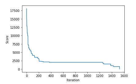
Running this, the main loop executed 1,541 times before finding a solution. Each iteration, it calls vary_policy() (described below) ten times to generate ten variations of the current policy. It then calls evaluate_policy() to evaluate each. This was defined above, and provides a score (in dollars), of how short the broker can come up using this policy in an average set of 128 instances of the world series (we can divide this by 128 to get the expected loss for any single world series). The lower the score, the better.
The initial solution had a score of 153,656.25, so quite poor, as expected. It rapidly improves from there, quickly dropping to around 100,000, then 70,000, then 50,000, and so on. Printing the best policies found to date as the code executes also presents increasingly more sensible policies.
Method to Generate Random Variations
The following code generates a single variation on the current policy:
def vary_policy(policy):
    new_policy = copy.deepcopy(policy)
    num_change = np.random.randint(1, 10)
    for _ in range(num_change):
        win_num = np.random.choice(4)
        game_num = np.random.choice(7)
        new_val = np.random.choice([x*31.25 for x in range(33)])
        new_policy[win_num][game_num] = new_val
    return new_policy
Here we first select the number of cells in the 4×7 policy to change, between 1 and 10. It’s possible to modify fewer cells, and this can improve performance when the scores are getting close to zero. That is, once we have a strong policy, we likely wish to change it less than we would near the beginning of the process, where the solutions tend to be weak and there is more emphasis on exploring the search space.
However, consistently modifying a small, fixed number of cells does allow getting stuck in local optima (sometimes there is no modification to a policy that modifies exactly, say, 1 or 2 cells that will work better, and it’s necessary to change more cells to see an improvement), and doesn’t always work well. Randomly selecting a number of cells to modify avoids this. Though, setting the maximum number here to ten is just for demonstration, and is not the result of any tuning.
If we were to limit ourselves to the 16 relevant cells of the 4×7 matrix for changes, this code would need only minor changes, simply skipping updates to those cells, and marking them with a special symbol (equivalent to ‘n/a’, such as np.NaN) for clarity when displaying the matrices.
Results
In the end, the algorithm was able to find the following policy. That is, in the first game, we will have no wins, so will bet $312.50. In the second game, we will have either zero or one win, but in either case will be $312.50. In the third game, we will have either zero, one, or two wins, so will bet $250, $375, or $250, and so on, up to, at most, seven games. If we reach game 7, we must have 3 wins, and will bet $1000 on that game.
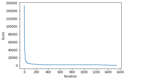
I’ve also created a plot of how the scores for the best policy found so far drops (that is, improves — smaller is better) over the 1,541 iterations:
The score for the best policy found so far over each of the iterations until a suitable solution (with a score of 0) is found.
This is a bit hard to see since the score is initially quite large, so we plot this again, skipping first 15 steps:
The score for the best policy found so far over each of the iterations (skipping the first 15 iterations) until a suitable solution (with a score of 0) is found.
We can see the score initially continuing to drop quickly, even after the first 15 steps, then going into a long period of little improvement until it eventually finds a small modification to the current policy that improves it, followed by more drops until we eventually reach a perfect score of 0 (being $0 short for any possible sequence of wins & losses).
Similar types of problems
The problem we worked on here is an example of what is known as a constraints satisfaction problem, where we simply wish to find a solution that covers all the given constraints (in this case, we take the constraints as hard constraints — it’s necessary to end correctly with either $0 or $2000 for any possible valid sequence of games).
Given two or more full solutions to the problem, there is no sense of one being better than the other; any that works is good, and we can stop once we have a workable policy. The N Queens problem and Sudoku, are two other examples of problems of this type.
Other types of problems may have a sense of optimality. For example, with the Travelling Salesperson Problem, any solution that visits every city exactly once is a valid solution, but each solution has a different score, and some are strictly better than others. In that type of problem, it’s never clear when we’ve reached the best possible solution, and we usually simply try for a fixed number of iterations (or amount of time), or until we’ve reached a solution with at least some minimal level of quality. Hill climbing can also be used with these types of problems.
It’s also possible to formulate a problem where it’s necessary to find, not just one, but all workable solutions. In the case of the Betting on World Series problem, it was simple to find a single workable solution, but finding all solutions would be much harder, requiring an exhaustive search (though optimized to quickly remove cases that are equivalent, or to quit evaluation early where policies have a clear outcome).
Similarly, we could re-formulate Betting on World Series problem to simply require a good, but not perfect, solution. For example, we could accept solutions where the broker comes out even most of the time, and only slightly behind in other cases. In that case, hill climbing can still be used, but something like a random search or grid search are also possible — taking the best policy found after a fixed number of trials, may work sufficiently in that case.
In problems harder than the Betting on World Series problem, simple hill climbing as we’ve used here may not be sufficient. It may be necessary, for example, to maintain a memory of previous policies, or to include a process called simulated annealing (where we take, on occasion, a sub-optimal next step — a step that may actually have lower quality than the current solution — in order to help break away from local optima).
For more complex problems, it may be better to use Bayesian Optimization, Evolutionary Algorithms, Particle Swarm Intelligence, or other more advanced methods. I’ll hopefully cover these in future articles, but this was a relatively simple problem, and straight-forward hill climbing worked quite well (though as indicated, can easily be optimized to work better).
Conclusions
This article provided a simple example of hill climbing. The problem was relatively straight-forward, so hopefully easy enough to go through for anyone not previously familiar with hill climbing, or as a nice example even where you are familiar with the technique.
What’s interesting, I think, is that despite this problem being solvable otherwise, optimization techniques such as used here are likely the simplest and most effective means to approach this. While tricky to solve otherwise, this problem was quite simple to solve using hill climbing.
We use cookies on our website to give you the most relevant experience by remembering your preferences and repeat visits. By clicking “Accept”, you consent to the use of ALL the cookies.
This website uses cookies to improve your experience while you navigate through the website. Out of these, the cookies that are categorized as necessary are stored on your browser as they are essential for the working of basic functionalities of the website. We also use third-party cookies that help us analyze and understand how you use this website. These cookies will be stored in your browser only with your consent. You also have the option to opt-out of these cookies. But opting out of some of these cookies may affect your browsing experience.
Necessary cookies are absolutely essential for the website to function properly. These cookies ensure basic functionalities and security features of the website, anonymously.
Cookie
Duration
Description
cookielawinfo-checkbox-analytics
11 months
This cookie is set by GDPR Cookie Consent plugin. The cookie is used to store the user consent for the cookies in the category "Analytics".
cookielawinfo-checkbox-functional
11 months
The cookie is set by GDPR cookie consent to record the user consent for the cookies in the category "Functional".
cookielawinfo-checkbox-necessary
11 months
This cookie is set by GDPR Cookie Consent plugin. The cookies is used to store the user consent for the cookies in the category "Necessary".
cookielawinfo-checkbox-others
11 months
This cookie is set by GDPR Cookie Consent plugin. The cookie is used to store the user consent for the cookies in the category "Other.
cookielawinfo-checkbox-performance
11 months
This cookie is set by GDPR Cookie Consent plugin. The cookie is used to store the user consent for the cookies in the category "Performance".
viewed_cookie_policy
11 months
The cookie is set by the GDPR Cookie Consent plugin and is used to store whether or not user has consented to the use of cookies. It does not store any personal data.
Functional cookies help to perform certain functionalities like sharing the content of the website on social media platforms, collect feedbacks, and other third-party features.
Performance cookies are used to understand and analyze the key performance indexes of the website which helps in delivering a better user experience for the visitors.
Analytical cookies are used to understand how visitors interact with the website. These cookies help provide information on metrics the number of visitors, bounce rate, traffic source, etc.
Advertisement cookies are used to provide visitors with relevant ads and marketing campaigns. These cookies track visitors across websites and collect information to provide customized ads.