
Practical techniques to accelerate heavy workloads with GPU optimization in Python
Originally appeared here:
How to Reduce Python Runtime for Demanding Tasks
Go Here to Read this Fast! How to Reduce Python Runtime for Demanding Tasks
Practical techniques to accelerate heavy workloads with GPU optimization in Python
Originally appeared here:
How to Reduce Python Runtime for Demanding Tasks
Go Here to Read this Fast! How to Reduce Python Runtime for Demanding Tasks

Most quick proof of concepts (POCs) which allow a user to explore data with the help of conversational AI simply blow you away. It feels like pure magic when you can all of a sudden talk to your documents, or data, or code base.
These POCs work wonders on small datasets with a limited count of docs. However, as with almost anything when you bring it to production, you quickly run into problems at scale. When you do a deep dive and you inspect the answers the AI gives you, you notice:
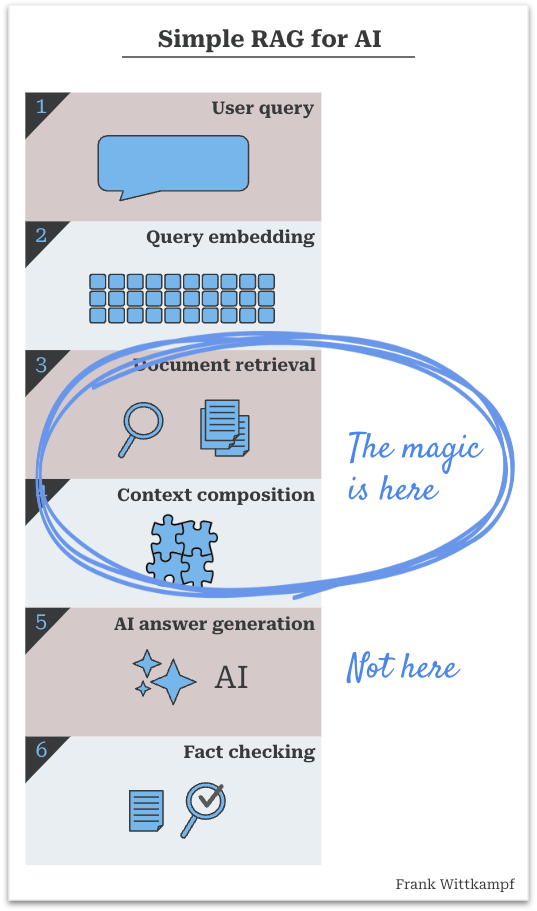
It turns out that the real magic in RAG does not happen in the generative AI step, but in the process of retrieval and composition. Once you dive in, it’s pretty obvious why…
* RAG = Retrieval Augmented Generation — Wikipedia Definition of RAG
A quick recap of how a simple RAG process works:
The dirty little secret is that the essence of the RAG process is that you have to provide the answer to the AI (before it even does anything), so that it is able to give you the reply that you’re looking for.
In other words:
Which is more important? The answer is, of course, it depends, because if judgement is the critical element, then the AI model does all the magic. But for an endless amount of business use cases, finding and properly composing the pieces that make up the answer, is the more important part.
The first set of problems to solve when running a RAG process are the data ingestion, splitting, chunking, document interpretation issues. I’ve written about a few of these in prior articles, but am ignoring them here. For now let’s assume you have properly solved your data ingestion, you have a lovely vector store or search index.
Typical challenges:
This list goes on, but you get the gist.
Short answer: no.
The cost and performance impact of using extremely large context windows shouldn’t be underestimated (you easily 10x or 100x your per query cost), not including any follow up interaction that the user/system has.
However, putting that aside. Imagine the following situation.
We put Anne in room with a piece of paper. The paper says: *patient Joe: complex foot fracture.* Now we ask Anne, does the patient have a foot fracture? Her answer is “yes, he does”.
Now we give Anne a hundred pages of medical history on Joe. Her answer becomes “well, depending on what time you are referring to, he had …”
Now we give Anne thousands of pages on all the patients in the clinic…
What you quickly notice, is that how we define the question (or the prompt in our case) starts to get very important. The larger the context window, the more nuance the query needs.
Additionally, the larger the context window, the universe of possible answers grows. This can be a positive thing, but in practice, it’s a method that invites lazy engineering behavior, and is likely to reduce the capabilities of your application if not handled intelligently.
As you scale a RAG system from POC to production, here’s how to address typical data challenges with specific solutions. Each approach has been adjusted to suit production requirements and includes examples where useful.
Duplication is inevitable in multi-source systems. By using fingerprinting (hashing content), document IDs, or semantic hashing, you can identify exact duplicates at ingestion and prevent redundant content. However, consolidating metadata across duplicates can also be valuable; this lets users know that certain content appears in multiple sources, which can add credibility or highlight repetition in the dataset.
# Fingerprinting for deduplication
def fingerprint(doc_content):
    return hashlib.md5(doc_content.encode()).hexdigest()

# Store fingerprints and filter duplicates, while consolidating metadata
fingerprints = {}
unique_docs = []
for doc in docs:
    fp = fingerprint(doc['content'])
    if fp not in fingerprints:
        fingerprints[fp] = [doc]
        unique_docs.append(doc)
    else:
        fingerprints[fp].append(doc)  # Consolidate sources
Near-duplicate documents (similar but not identical) often contain important updates or small additions. Given that a minor change, like a status update, can carry critical information, freshness becomes crucial when filtering near duplicates. A practical approach is to use cosine similarity for initial detection, then retain the freshest version within each group of near-duplicates while flagging any meaningful updates.
from sklearn.metrics.pairwise import cosine_similarity
from sklearn.cluster import DBSCAN
import numpy as np

# Cluster embeddings with DBSCAN to find near duplicates
clustering = DBSCAN(eps=0.1, min_samples=2, metric="cosine").fit(doc_embeddings)

# Organize documents by cluster label
clustered_docs = {}
for idx, label in enumerate(clustering.labels_):
 if label == -1:
 continue
 if label not in clustered_docs:
 clustered_docs[label] = []
 clustered_docs[label].append(docs[idx])

# Filter clusters to retain only the freshest document in each cluster
filtered_docs = []
for cluster_docs in clustered_docs.values():
 # Choose the document with the most recent timestamp or highest relevance
 freshest_doc = max(cluster_docs, key=lambda d: d['timestamp'])
 filtered_docs.append(freshest_doc)
When a query returns a high volume of relevant documents, effective handling is key. One approach is a **layered strategy**:
This approach reduces the workload by retrieving synthesized information that’s more manageable for the AI. Other strategies could involve batching documents by theme or pre-grouping summaries to further streamline retrieval.
Balancing quality with freshness is essential, especially in fast-evolving datasets. Many scoring approaches are possible, but here’s a general tactic:
Other strategies could involve scoring only high-quality sources or applying decay factors to older documents.
Ensuring diverse data sources in retrieval helps create a balanced response. Grouping documents by source (e.g., different databases, authors, or content types) and selecting top snippets from each source is one effective method. Other approaches include scoring by unique perspectives or applying diversity constraints to avoid over-reliance on any single document or perspective.
# Ensure variety by grouping and selecting top snippets per source

from itertools import groupby

k = 3  # Number of top snippets per source
docs = sorted(docs, key=lambda d: d['source'])

grouped_docs = {key: list(group)[:k] for key, group in groupby(docs, key=lambda d: d['source'])}
diverse_docs = [doc for docs in grouped_docs.values() for doc in docs]
Ambiguous queries can lead to suboptimal retrieval results. Using the exact user prompt is mostly not be the best way to retrieve the results they require. E.g. there might have been an information exchange earlier on in the chat which is relevant. Or the user pasted a large amount of text with a question about it.
To ensure that you use a refined query, one approach is to ensure that a RAG tool provided to the model asks it to rephrase the question into a more detailed search query, similar to how one might carefully craft a search query for Google. This approach improves alignment between the user’s intent and the RAG retrieval process. The phrasing below is suboptimal, but it provides the gist of it:
tools = [{
  "name": "search_our_database",
  "description": "Search our internal company database for relevent documents",
  "parameters": {
   "type": "object",
   "properties": {
    "query": {
     "type": "string",
     "description": "A search query, like you would for a google search, in sentence form. Take care to provide any important nuance to the question."
    }
   },
   "required": ["query"]
  }
}]
For tailored responses, integrate user-specific context directly into the RAG context composition. By adding a user-specific layer to the final context, you allow the AI to take into account individual preferences, permissions, or history without altering the core retrieval process.
By addressing these data challenges, your RAG system can evolve from a compelling POC into a reliable production-grade solution. Ultimately, the effectiveness of RAG relies more on careful engineering than on the AI model itself. While AI can generate fluent answers, the real magic lies in how well we retrieve and structure information. So the next time you’re impressed by an AI system’s conversational abilities, remember that it’s likely the result of an expertly designed retrieval process working behind the scenes.
I hope this article provided you some insight into the RAG process, and why the magic that you experience when talking to your data isn’t necessarily coming from the AI model, but is largely dependent on the design of your retrieval process.
Please comment with your thoughts.
Spoiler Alert: The Magic of RAG Does Not Come from AI was originally published in Towards Data Science on Medium, where people are continuing the conversation by highlighting and responding to this story.
Originally appeared here:
Spoiler Alert: The Magic of RAG Does Not Come from AI
Go Here to Read this Fast! Spoiler Alert: The Magic of RAG Does Not Come from AI

Automatic music transcription is the process of converting audio files like MP3 and WAV into sheet music, guitar tablature, and any format a musician may want to learn a song on their instrument.
We’ll go over the best current tools for doing this, which happen to be deep learning-based, and a novel approach for it.
The current state-of-the-art for this task comes from Magenta, an open-source research project developed by the now defunct (as of April 2023) Google Brain Team.
They released a paper Sequence-to-Sequence Piano Transcription with Transformers in 2021 which used a T5-inspired transformer model (similar to “t5-small”) with 54 million parameters and the Maestro dataset, achieving great results. The problem is approached as a sequence-to-sequence task using an encoder-decoder Transformer architecture. The encoder processes mel spectrogram frames as input and produces embeddings, while the decoder uses these embeddings via cross-attention to autoregressively generate a sequence of MIDI-like tokens. Their vocabulary consisted of four types of tokens:
See the image below for a visualisation of the architecture and an example sequence of their custom MIDI tokens:
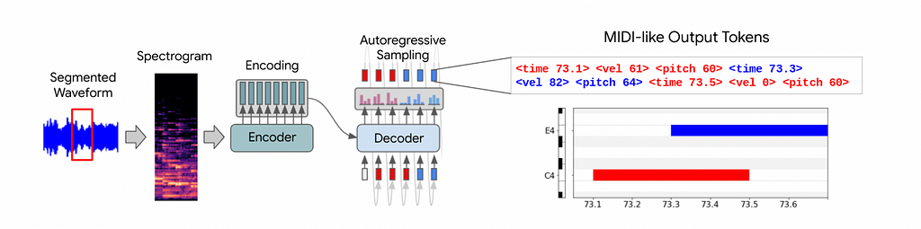
Our model is a generic encoder-decoder Transformer architecture where each input position contains a single spectrogram frame and each output position contains an event from our MIDI-like vocabulary. Outputs tokens are autoregressively sampled from the decoder, at each step taking the token with maximum probability.
In 2022, they released a paper, MT3: Multi-Task Multitrack Music Transcription. This experiment used the same approach as the last one but added additional instrument tokens to represent the different instruments. Again, they used a similar T5 model and achieved great performance against many of the datasets trained on, notably Slakh, Maestro and MusicNet.
MR-MT3 was released the following year as a slight improvement to MT3.
Huge resources were needed to train this from scratch, despite being much smaller in size compared to even the smallest language models. The 2021 paper noted:
“We trained all models on 32 TPUv3 cores, resulting in a per-core batch size of 8. Based on validation set results, overfitting did not seem to be a problem, so we allowed training to progress for 400K steps, which took about 2.5 days for our baseline models.”
The MT3 paper doesn’t provide as specific details on training, stating they train for 1 million steps.
These models have some inherent limitations in their output flexibility. While language models typically have large vocabularies (often 30,000+ tokens) that are extensively pre-trained on diverse natural language data, MT3 and similar music transcription models use a much smaller, specialised token vocabulary (only a few thousand tokens) focused solely on musical events. This specialisation means that adding new tokens, such as for new instruments or playing techniques like palm muting on guitars or pizzicato on violins, is likely not easy — it requires significant retraining to integrate these new tokens effectively with the existing vocabulary, and often requires substantial training data demonstrating these techniques. This differs from large language models which can often describe such musical nuances in natural language without modification, as they’ve encountered these concepts during their broad pre-training.
We can leverage transfer learning from large open-source pre-trained audio and language models. Examples of music generation models include OpenAI’s Jukebox and Meta’s MusicGen.
GPT-4o is designed to handle text, audio and images “natively”. Although OpenAI has not released the technical details on this, it’s assumed that some weights in the network will process all modalities. It’s possible that the model uses a decoder-only architecture like language only GPT models without the need for encoder components to convert different modalities to a dense representation first. This design allows the model to seamlessly process and interpret inputs like text and images together, potentially offering performance benefits both computationally and in terms of model understanding.
Many multi-modal models take a simpler approach reminiscent of the encoder-decoder architecture: they combine two pre-trained models — an encoder for the specific input modality (like ViT for vision or an audio encoder for sound) and a Large Language Model (such as LLaMA, Gemma, or Qwen). These models are connected through projection layers that align their representations in a shared latent space, often using just a single linear layer. These projection layers learn to convert the encoder’s output into a format that matches the LLM’s expected input dimensions and characteristics. The projection creates new embeddings/tokens from the input modality that can then be injected into the LLM’s input sequence. LLaVA is a prime example of this architecture for vision-language tasks, while Spotify’s Llark and Qwen-Audio apply the same principle using audio encoders instead of vision encoders.
Here’s some pseudocode on how the models are stitched together:
# Extract features from final layer of audio encoder
# Shape: [batch_size, audio_seq_len, encoder_dim=1024]
audio_features = audio_model(audio_input)

# Project audio features to match LLM's embedding dimension
# Shape: [batch_size, audio_seq_len, llm_embed_dim=4096]
audio_embeddings = projection_layer(audio_features)

# Get text embeddings from LLM's embedding layer
# Shape: [batch_size, text_seq_len, llm_embed_dim=4096]
text_embeddings = llm.embed_text(text_input)

# Concatenate along sequence length dimension
# Shape: [batch_size, audio_seq_len + text_seq_len, llm_embed_dim=4096]
combined_input = concatenate([audio_embeddings, text_embeddings], dim=1)

# Feed them into the LLM as normal for generation
output = llm(combined_input)
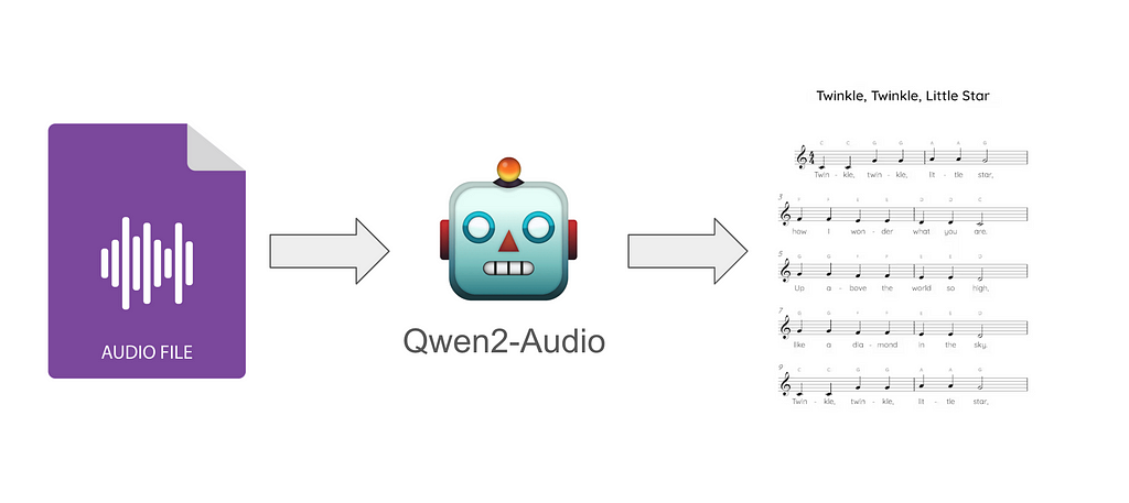
Llark uses OpenAI’s Jukebox and Qwen2-Audio uses OpenAI’s Whisper for the audio towers. Jukebox is a music generation model but it can also take in audio clips as input and outputs a continuation of the audio clip. Whisper is used for transcribing voice to text.
Given their purpose, the choice of audio module is clear: Llark specialises in music analysis, while Qwen2Audio primarily focuses on responding to voice instructions with some basic audio and music analysis capabilities.
Determining the optimal source for extracting embeddings from large pre-trained models involves research and experimentation. Additionally, deciding whether to fine-tune the entire module or freeze parts of it is a crucial design choice. For instance, LlaVa’s training strategy involves freezing the vision tower and focusing on fine-tuning the projection layer and language model. We’ll go over this aspect of each model below.
Determining the optimal location to extract embeddings from large models typically requires extensive probing. This involves testing various activations or extracted layers of the model on different classification tasks through a process of trial and error. For music generation models, this could include tasks like genre recognition, instrument detection, emotion detection, as well as analysis of harmonic structures and temporal patterns. Many commercial embedding models (like OpenAI’s embedding models) are trained specifically for embedding generation with specialised architectures and training objectives, rather than being fine-tuned versions of existing language models.
The two largest publicly available music generation and music continuation (i.e.: able to take in audio as input) models are Jukebox and MusicGen. MusicGen is newer and faster, and therefore seemed like it would be the obvious choice to me. However, according to this paper on probing MusicGen, embeddings extracted from Jukebox appear to outperform MusicGen on average in classification tasks. The findings from this paper led to the authors of Llark using the following approach for extracting embeddings:
(The downsampled embedding size is approximately 6x larger than CLIP ViT-L14 models used in many multimodal vision models)
The embedding extraction for Qwen2Audio isn’t mentioned in detail in the paper. Whisper is an encoder-decoder architecture where the encoder generates deeply learned representations of the audio and the decoder decodes the representations to text (the transcription). In Qwen2Audio, it appears they extract embeddings from the final layer of Whisper’s encoder, although they don’t mention whether they freeze it during training.
Unfortunately Spotify has not provided any datasets or their trained model weights to the public, noting:
“With respect to inputs: the inputs to our model are public, open-source, Creative Commons-licensed audio and associated annotations. However, each individual audio file can have its own, potentially more restrictive license. Many of the audio files include “no derivatives” licenses. We encourage users of the datasets to familiarize themselves with the restrictions of these licenses; in order to honor such licenses, we do not release any derivatives from the training data in this paper (including query- response pairs or trained model weights).”
They used the following datasets:
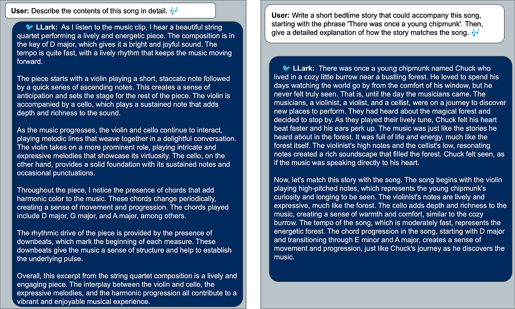
Llark details it’s training data generation process in the following extract:
“We use variants of ChatGPT to extract the instruction- tuning data for all experiments. However, the exact language model used varies by dataset. We select the OpenAI model as follows: We use GPT-4 for all reasoning tasks. We found that GPT-4 was much more adept at following the complex instructions in the Reasoning task family. For datasets with more than 25k samples, we limit Reasoning data to a random subsample of 25k tracks.”
This results in Q&A data like this:
The datasets used for training Qwen2Audio are not shared either, but the trained model is widely available and also is implemented in the transformers library:
For this project, fine-tuning off a pre-trained Llark model would have been optimal, given it’s reportedly good performance against the evaluation benchmarks Spotify stated in the paper.
However, given they didn’t release the weights for it, it’s unfeasible to start training a model like this from scratch without a fair bit of expertise and money. Spotify trained it on:
Our model is trained on 4 80GB NVIDIA A100 GPUs. Training takes approximately 54 hours.
This would cost around $700 using a provider like LambdaLabs.
Because of the above, I went with Qwen. However, Qwen2-Audio doesn’t perform that well across basic music tasks like tempo and instrument detection. I detail this below in the evaluation section. This means that the model is probably not large enough or pre-trained enough to achieve this task, but my hope is I could at least set a starting point and framework for fine-tuning on this task in the future. As Alibaba state in their Qwen2-Audio blog post:
We also plan to build larger Qwen2-Audio models to explore the scaling laws of audio language models.
For my own learning though, I did have a go at re-creating the model using torch and pre-trained models with the transformers library.
I also created datasets for Q&A data and embeddings. I generated short form Q&A data for the URMP dataset, e.g.: “What is the tempo of this track”, “What instruments are playing in this audio”.
Here’s a notebook for running Jukebox in a Colab environment to take advantage of the cheap T4 GPU’s. I uploaded both Q&A and embeddings datasets to HuggingFace here.
Here’s a notebook with Llark replicated.
I chose ABC music notation as the output format that the language model is expected to transcribe the music in. Here’s an example of it:
X:1
M:4/4
L:1/16
K:none
Q:67

V:1 name="Electric Bass (finger)"
%%octave-default C4
GAA^2E3A2<A^2 | D^D^2E2A2A^4 A^2E2 | A2A^4A^2E2 A2A^4 | A^2E2A2A^4A^2E2A2 |
A^4 A^2E2 A2A^4A^2 E2 | A2A^4 |

V:2 name="Bright Acoustic Piano"
%%octave-default C5
[E3C3][E3C3][E3C3] [E3C3][A^,2E2A^2] | [E3A^3][E3A^3][E3A^3][E3A^3][E3A^3] |
[E3A^3][E3A^3][E3A^3] [E3A^3][E3A^3] | [E3A^3][E3A^3][E3A^3][E3A^3][E3A^3] |
[E3A^3][E3A^3][E3A^3] [E3A^3][E3A^3] | [E3A^3] |

V:3 name="Electric Guitar (jazz)"
%%octave-default C5
E'3C'3A^4E'3C'3 | A^4E'3 C'3A^4E'3C'3 | A^4 E'3C'3A^4 E'3C'3 | A^4E'3C'3A^4E'3C'3 |
A^4E'3C'3 A^4E'3C'3 | A^4 |
In this notation we have the time signature and tempo defined at the top denoted by ‘M’ and ‘Q’. The ‘L’ indicates the default note length of the notation, in this case a sixteenth note, which is the norm. We then define each instrument and the default octave they should adhere to when writing the notes for each of them. Here’s a summary of the key syntactical points for writing notes in ABC music notation:
The reasons for choosing this notation are:
I converted the MIDI files provided by the datasets to ABC notation using this library. A notebook for creating the datasets is here.
To evaluate both the original model and each stage of fine-tuning I performed thereafter, I randomly selected 30 samples of varying complexity from the URMP dataset and ran the model three times on each sample, manually examining all responses.
Through manual testing, I found the optimal decoding parameters to be a temperature of 0.7 and a top_p of 1.2. The maximum number of tokens to return was capped at 2048. Adjusting the max seemed to have little difference on performance.
The original model performed poorly on this evaluation set. While it occasionally predicted the tempo and instruments correctly, it mostly failed to do so. A text file with the evaluation results is available here.
Given this starting point, it’s unlikely that we’ll see strong results from this experiment without a robust pre-trained model. However, the goal is to develop strategies that can be applied in the future as more advanced pre-trained models become available.
I first attempted fine-tuning with basic cross-entropy loss. Supervised fine-tuning with cross-entropy loss is a quick way to start teaching the model but a basic loss function like this has limitations as we will see below. The intuition behind this stage of training is that it would nudge the model in the right direction and it would pick up any patterns or any customised ABC notation the dataset may have which the model may not have seen before.
First, we trained it in a typical supervised fine-tuning manner for language models. I used the SFTtrainer from the trl library for this, which uses cross-entropy loss with teacher forcing defined step by step below:
The results from this training phase were poor. It degraded the performance of the original model. The model, which previously handled tempo and instrument recognition well, now mostly got these wrong. It also began producing garbled text output with endless repetition. This occurred even when setting a low learning rate, applying gradient clipping, and using low LoRA ranks to mitigate large changes to the model. Overall, it seemed the model was very sensitive to the training applied.
However, while this training phase may offer some improvements, it won’t lead to optimal performance due to the limitations of our basic loss function. This function struggles to fully capture the model’s performance nuances. For example, when using teacher forcing, instrument predictions can yield deceptively low loss across certain token sections. If an instrument name begins with “V”, the model might confidently predict “Violin” or “Viola” based on our dataset, regardless of accuracy. Additionally, the loss function may not accurately reflect near-misses, such as predicting a tempo of 195 instead of 200 — a small difference that’s reasonably accurate but potentially penalised heavily dependent on the distribution of probabilities amongst logits. It’s possible that neighbouring numbers also have high probabilities.
Because of these limitations, we can create our own custom loss function that can more accurately score the response from the model. That is, given a predicted sequence from the model, the loss function could give it a score between 0 and 1 on how good it is.
However, integrating this custom loss function into supervised fine-tuning presents a significant challenge. The issue stems from the non-linearity introduced by the custom loss function, which prevents the direct calculation of gradients. Let’s break this down:
In traditional SFT with cross-entropy loss:
With our custom loss function:
To overcome this, reinforcement learning techniques like Proximal Policy Optimisation (PPO) can be employed. PPO is specifically designed to handle non-differentiable loss functions and can optimise the model by considering the entire policy (the model’s output distribution), rather than relying on gradient information from logits.
Note, there’s a lot of great articles on here explaining PPO!
The key insight of PPO is that instead of trying to directly backpropagate through the non-differentiable steps, it:
This approach allows us to effectively train the model with the custom loss function, ensuring performance improvements without disrupting the core training dynamics. The PPO algorithm’s conservative update strategy helps maintain stability during training, which is particularly important when working with large language models.
Usually, this scoring function would be implemented as a separate LLM in the form of a “reward model” commonly used when fine-tuning models via RLHF, which was a breakthrough first introduced when ChatGPT came out. Due to the nature of this task, we can manually write code to score the responses, which uses fewer resources and is quicker.
For time signature and tempo recognition this is easy to calculate. We extract all predicted items with regex, for example extracting the metre:
def extract_metre(self, abc_string):
  return re.search(r'M:(S+)', abc_string).group(1)
The model should learn the syntax and structure we want it to output in the SFT stage. If it outputs something that will cause our regex to not find anything or error, we can just skip that sample, assuming it’s a small minority of the dataset.
We extract the predicted tempo and write a function that is more forgiving for small errors but penalises larger errors more heavily:
Let’s break down the key components of this custom loss:
Code for the custom loss is here
1. Metre Loss
The metre loss focuses on the time signature of the piece. It compares the predicted metre with the ground truth, considering both the numerator and denominator separately, as well as their ratio. This approach allows for a nuanced evaluation that can handle various time signatures accurately.
The metre loss uses a combination of linear and exponential scaling to penalise differences. Small discrepancies result in a linear increase in loss, while larger differences lead to an exponential increase, capped at a maximum value of 1.
2. Tempo Loss
Tempo loss evaluates the accuracy of the predicted beats per minute (BPM). Similar to the metre loss, it uses a combination of linear and exponential scaling.
For small tempo differences (≤10 BPM), the function applies linear scaling. Larger differences trigger exponential scaling, ensuring that significant tempo mismatches are penalised more heavily.
3. Pitch Loss
The pitch loss is perhaps the most crucial component, as it assesses the accuracy of the transcribed notes. This function uses the Levenshtein distance to compare the sequence of notes in each voice.
The pitch loss calculation accounts for multiple voices, matching each predicted voice to the closest ground truth voice. This approach allows for flexibility in voice ordering while still maintaining accuracy in the overall pitch content.
4. Instrument Loss
The instrument loss evaluates the accuracy of instrument selection for each voice.
This function considers exact matches, instruments from the same family, and uses string similarity for more nuanced comparisons. It provides a comprehensive assessment of how well the model identifies and assigns instruments to each voice.
5. Combining the Losses
The final loss is a weighted combination of these individual components:
total_loss = (0.5 * pitch_loss +
 0.15 * metre_loss +
 0.15 * tempo_loss +
 0.2 * instrument_loss)
This weighting scheme prioritises pitch accuracy while still considering other important aspects of music transcription.
PPO training generally requires a lot more memory than SFT for a few reasons:
Because of the above, we’re more limited than SFT in the size of the models we can train and how much it costs. Whereas the above training I could do on an A100 40GB in Colab, for the PPO training I needed more memory. I trained on an H100 80GB, which could train a LoRA with a rank of 128 and a batch size of 8.
My hyperparameter sweep was narrow, I went with what seemed most intuitive using batch sizes ranging from 1 to 16 and learning rates from 2e-5 to 2e-4.
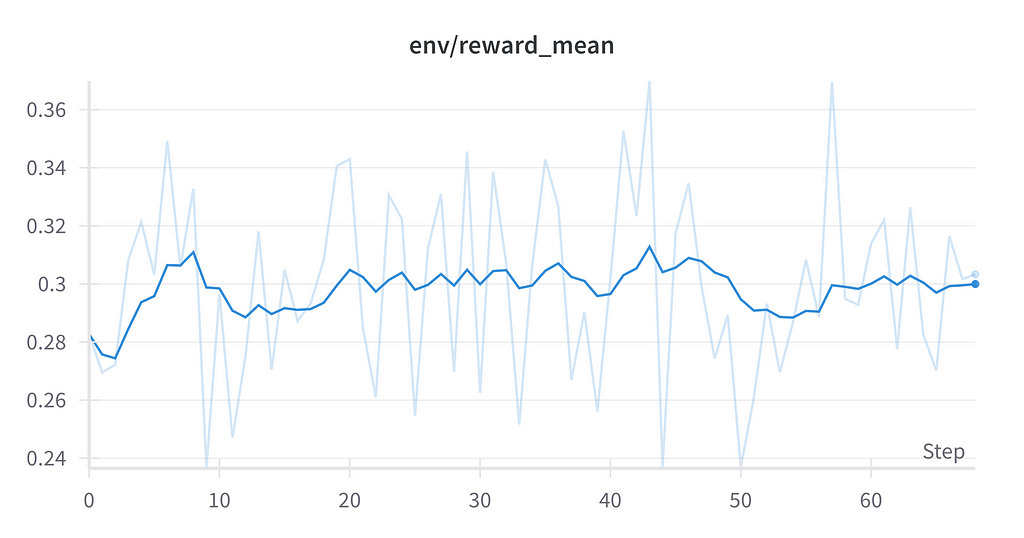
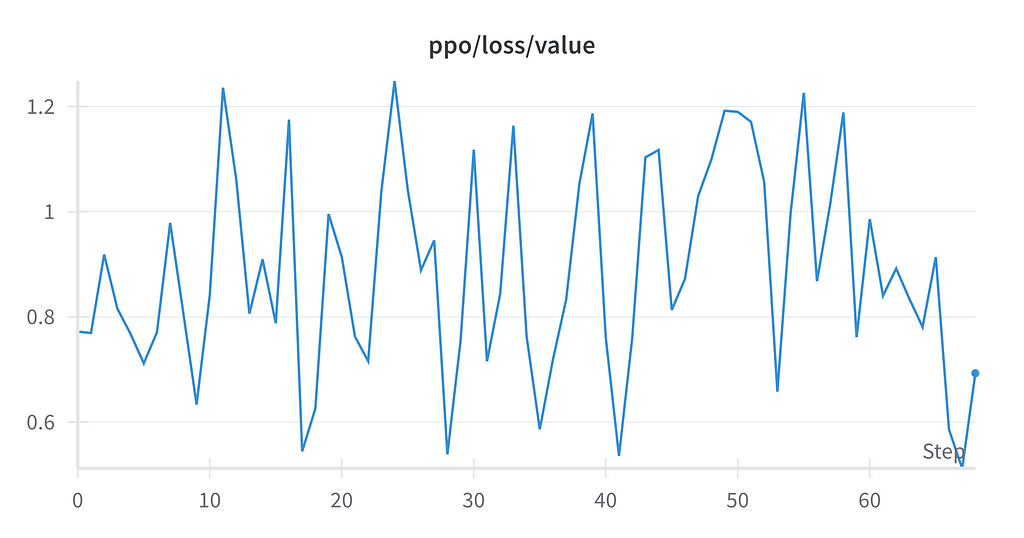
The model made no improvements to the task. The text file with the results is here.
I tracked various training metrics using Weights & Biases (WandB). Key metrics included the policy loss, value loss, total loss, KL divergence, and the reward model’s score.
For all hyperparameter runs, the logs no improvement in the rewards and loss calculated over time. The KL divergence remained within the pre-defined threshold.
While this initial experiment didn’t achieve the desired performance in music transcription, we’ve provided some groundwork for future developments in the space. The challenges encountered have provided valuable insights into both the technical requirements and potential approaches for tackling this complex task. Future work could explore several promising directions:
Here’s my notebook for running these experiments with Qwen2-Audio!
Exploring Music Transcription with Multi-Modal Language Models was originally published in Towards Data Science on Medium, where people are continuing the conversation by highlighting and responding to this story.
Originally appeared here:
Exploring Music Transcription with Multi-Modal Language Models
Go Here to Read this Fast! Exploring Music Transcription with Multi-Modal Language Models


A deep dive into LLM visualization and interpretation using sparse autoencoders
Originally appeared here:
Open the Artificial Brain: Sparse Autoencoders for LLM Inspection
Go Here to Read this Fast! Open the Artificial Brain: Sparse Autoencoders for LLM Inspection
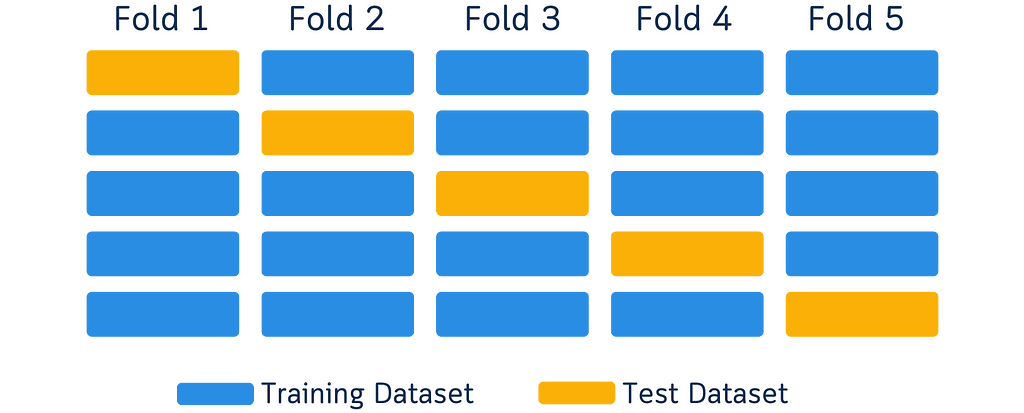

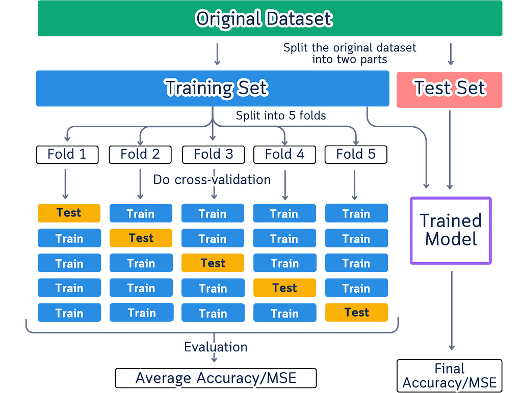
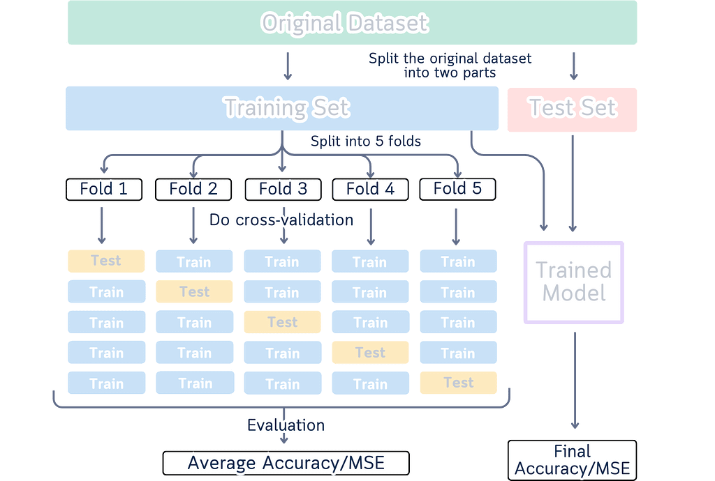
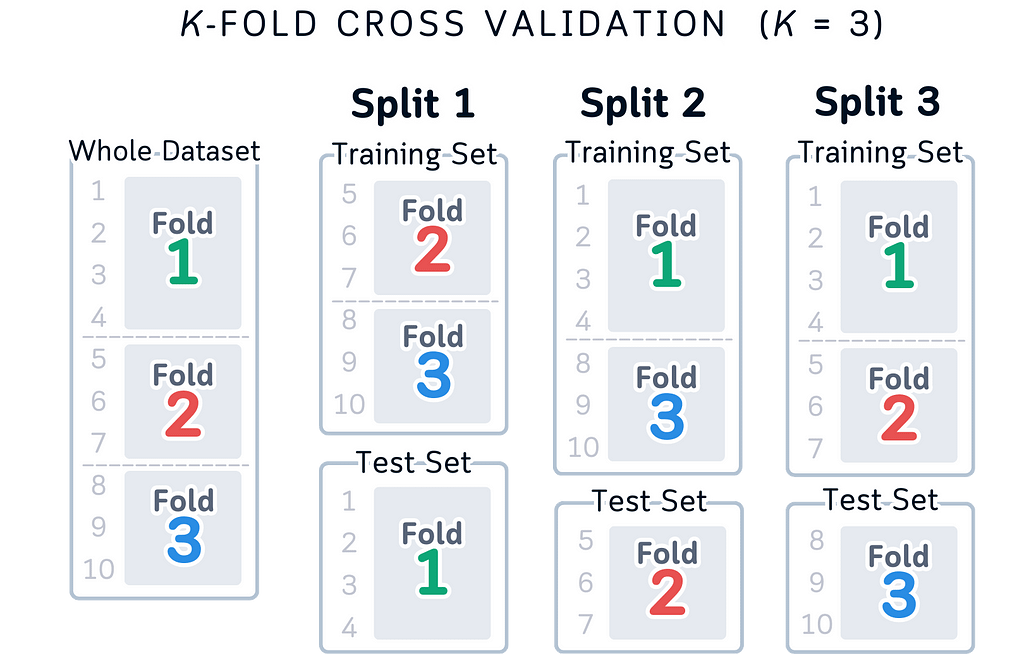
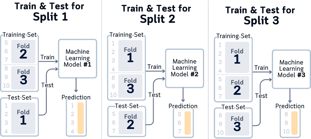
You know those cross-validation diagrams in every data science tutorial? The ones showing boxes in different colors moving around to explain how we split data for training and testing? Like this one:
I’ve seen them too — one too many times. These diagrams are common — they’ve become the go-to way to explain cross-validation. But here’s something interesting I noticed while looking at them as both a designer and data scientist.
When we look at a yellow box moving to different spots, our brain automatically sees it as one box moving around.
It’s just how our brains work — when we see something similar move to a new spot, we think it’s the same thing. (This is actually why cartoons and animations work!)
But here’s the thing: In these diagrams, each box in a new position is supposed to show a different chunk of data. So while our brain naturally wants to track the boxes, we have to tell our brain, “No, no, that’s not one box moving — they’re different boxes!” It’s like we’re fighting against how our brain naturally works, just to understand what the diagram means.
Looking at this as someone who works with both design and data, I started thinking: maybe there’s a better way? What if we could show cross-validation in a way that actually works with how our brain processes information?

Cross-validation is about making sure machine learning models work well in the real world. Instead of testing a model once, we test it multiple times using different parts of our data. This helps us understand how the model will perform with new, unseen data.
Here’s what happens:
The goal is to get a reliable understanding of our model’s performance. That’s the core idea — simple and practical.
(Note: We’ll discuss different validation techniques and their applications in another article. For now, let’s focus on understanding the basic concept and why current visualization methods need improvement.)
Open up any machine learning tutorial, and you’ll probably see these types of diagrams:
Here are the issues with such diagram:
Colors create practical problems when showing data splits. Some people can’t differentiate certain colors, while others may not see colors at all. The visualization fails when printed in black and white or viewed on different screens where colors vary. Using color as the primary way to distinguish data parts means some people miss important information due to their color perception.
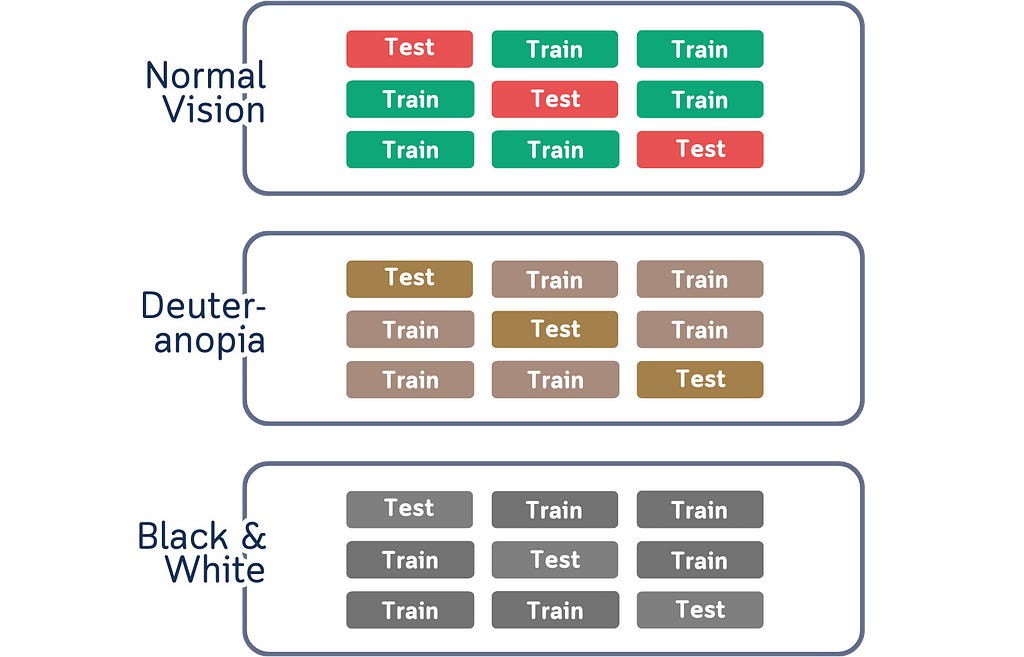
Another thing about colors is that it might look like they help explain things, but they actually create extra work for our brain. When we use different colors for different parts of the data, we have to actively remember what each color represents. This becomes a memory task instead of helping us understand the actual concept. The connection between colors and data splits isn’t natural or obvious — it’s something we have to learn and keep track of while trying to understand cross-validation itself.
Our brain doesn’t naturally connect colors with data splits.
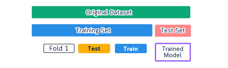
The current diagrams also suffer from information overload. They attempt to display the entire cross-validation process in a single visualization, which creates unnecessary complexity. Multiple arrows, extensive labeling, all competing for attention. When we try to show every aspect of the process at the same time, we make it harder to focus on understanding each individual part. Instead of clarifying the concept, this approach adds an extra layer of complexity that we need to decode first.
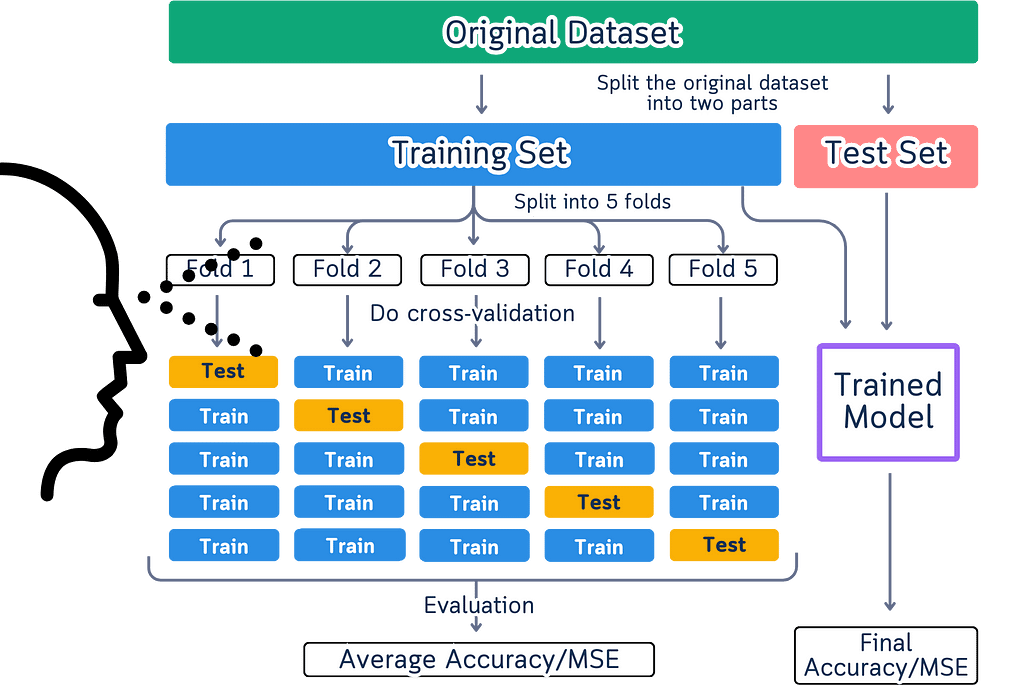
Movement in these diagrams creates a fundamental misunderstanding of how cross-validation actually works. When we show arrows and flowing elements, we’re suggesting a sequential process that doesn’t exist in reality. Cross-validation splits don’t need to happen in any particular order — the order of splits doesn’t affect the results at all.
These diagrams also give the wrong impression that data physically moves during cross-validation. In reality, we’re simply selecting different rows from our original dataset each time. The data stays exactly where it is, and we just change which rows we use for testing in each split. When diagrams show data flowing between splits, they add unnecessary complexity to what should be a straightforward process.
We need diagrams that:
Let’s fix this. Instead of trying to make our brains work differently, why don’t we create something that feels natural to look at?
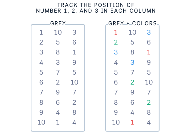
Let’s try something different. First, this is how data looks like to most people — rows and columns of numbers with index.
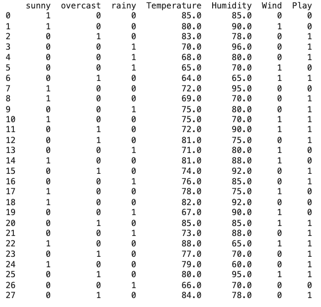
Inspired by that structure, here’s a diagram that make more sense.
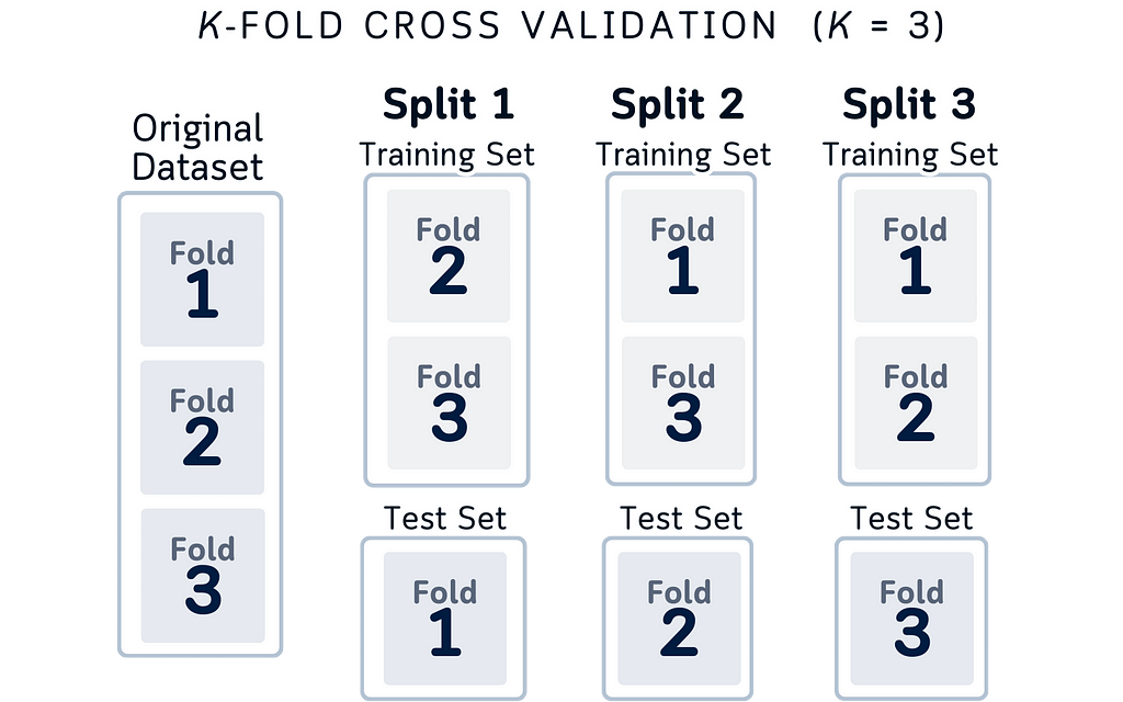
Here’s why this design makes more sense logically:
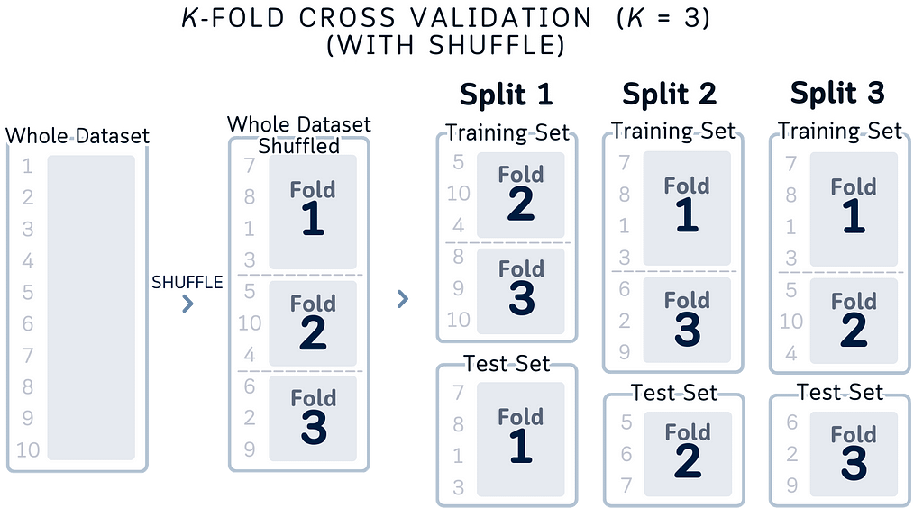
While the concept above is correct, thinking about actual row indices makes it even clearer:
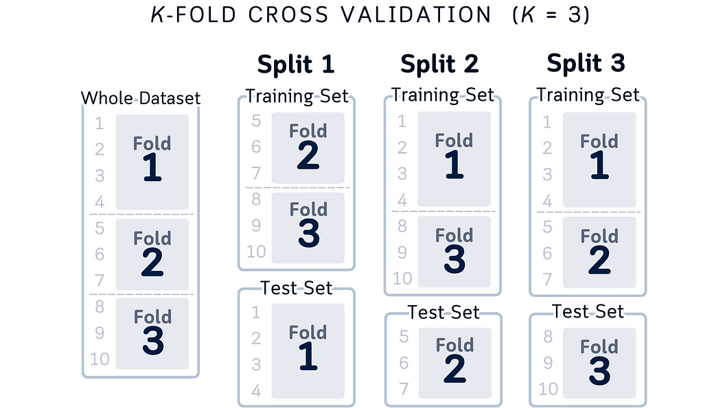
Here are some reasons of improvements of this visual:
This index-based view doesn’t change the concepts — it just makes them more concrete and easier to implement in code. Whether you think about it as portions or specific row numbers, the key principles remain the same: independent folds, complete coverage, and using all your data.
If you feel the black-and-white version is too plain, this is also another acceptable options:
While using colors in this version might seem problematic given the issues with color blindness and memory load mentioned before, it can still work as a helpful teaching tool alongside the simpler version.
The main reason is that it doesn’t only use colors to show the information — the row numbers (1–10) and fold numbers tell you everything you need to know, with colors just being a nice extra touch.
This means that even if someone can’t see the colors properly or prints it in black and white, they can still understand everything through the numbers. And while having to remember what each color means can make things harder to learn, in this case you don’t have to remember the colors — they’re just there as an extra help for people who find them useful, but you can totally understand the diagram without them.
Just like the previous version, the row numbers also help by showing exactly how the data is being split up, making it easier to understand how cross-validation works in practice whether you pay attention to the colors or not.
The visualization remains fully functional and understandable even if you ignore the colors completely.
Let’s look at why our new designs makes sense not just from a UX view, but also from a data science perspective.
Matching Mental Models: Think about how you explain cross-validation to someone. You probably say “we take these rows for testing, then these rows, then these rows.” Our visualization now matches exactly how we think and talk about the process. We’re not just making it pretty, we’re making it match reality.
Data Structure Clarity: By showing data as columns with indices, we’re revealing the actual structure of our dataset. Each row has a number, each number appears in exactly one test set. This isn’t just good design, it’s accurate to how our data is organized in code.
Focus on What Matters: Our old way of showing cross-validation had us thinking about moving parts. But that’s not what matters in cross-validation. What matters is:
Our new design answers these questions at a glance.
Index-Based Understanding: Instead of abstract colored boxes, we’re showing actual row indices. When you write cross-validation code, you’re working with these indices. Now the visualization matches your code — Fold 1 uses rows 1–4, Fold 2 uses 5–7, and so on.
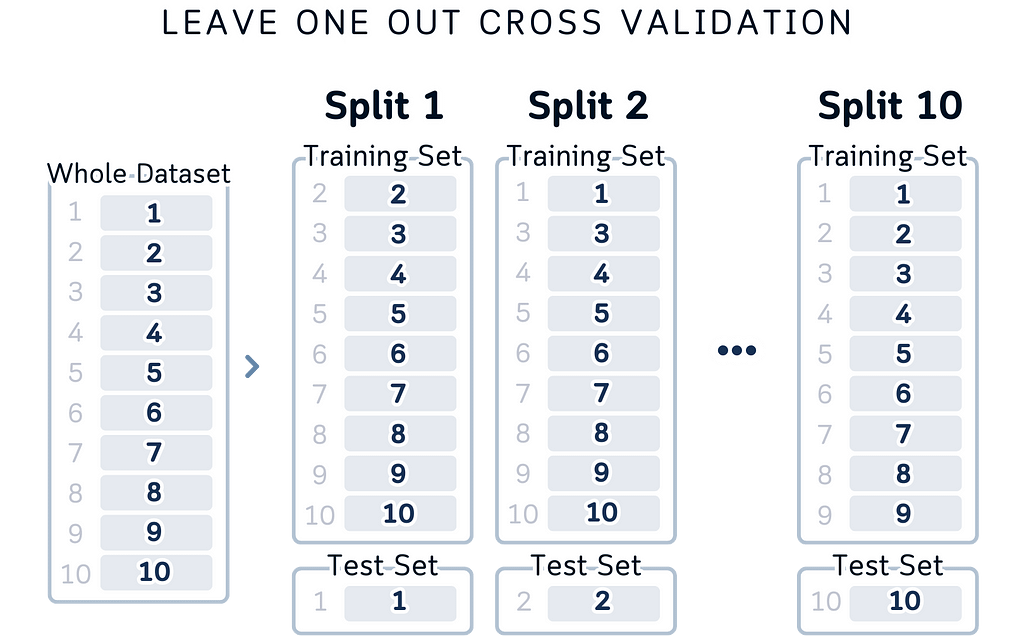
Clear Data Flow: The layout shows data flowing from left to right: here’s your dataset, here’s how it’s split, here’s what each split looks like. It matches the logical steps of cross-validation and it’s also easier to look at.
Here’s what we’ve learned about the whole redrawing of the cross-validation diagram:
Match Your Code, Not Conventions: We usually stick to traditional ways of showing things just because that’s how everyone does it. But cross-validation is really about selecting different rows of data for testing, so why not show exactly that? When your visualization matches your code, understanding follows naturally.
Data Structure Matters: By showing indices and actual data splits, we’re revealing how cross-validation really works while also make a clearer picture. Each row has its place, each split has its purpose, and you can trace exactly what’s happening in each step.
Simplicity Has It Purpose: It turns out that showing less can actually explain more. By focusing on the essential parts — which rows are being used for testing, and when — we’re not just simplifying the visualization but we’re also highlighting what actually matters in cross-validation.
Looking ahead, this thinking can apply to many data science concepts. Before making another visualization, ask yourself:
Good visualization isn’t about following rules — it’s about showing truth. And sometimes, the clearest truth is also the simplest.
Unless otherwise noted, all images are created by the author, incorporating licensed design elements from Canva Pro.
Why Most Cross-Validation Visualizations Are Wrong (And How to Fix Them) was originally published in Towards Data Science on Medium, where people are continuing the conversation by highlighting and responding to this story.
Originally appeared here:
Why Most Cross-Validation Visualizations Are Wrong (And How to Fix Them)
Go Here to Read this Fast! Why Most Cross-Validation Visualizations Are Wrong (And How to Fix Them)


Can Quantum Computing help improving our ability to train Large Neural Networks encoding language models (LLMs)?
Originally appeared here:
Of LLMs, Gradients, and Quantum Mechanics
Go Here to Read this Fast! Of LLMs, Gradients, and Quantum Mechanics


Watch out for these three ways too much of a good thing can be dangerous
Originally appeared here:
ROI Worship Can Be Bad For Business
Go Here to Read this Fast! ROI Worship Can Be Bad For Business
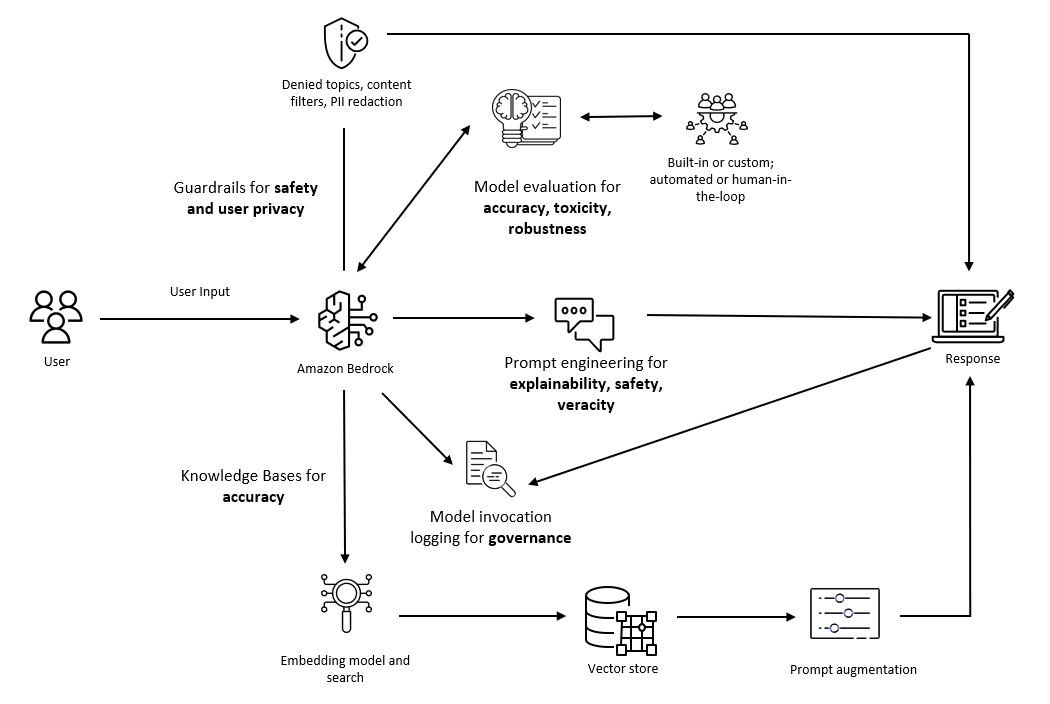

Originally appeared here:
Considerations for addressing the core dimensions of responsible AI for Amazon Bedrock applications
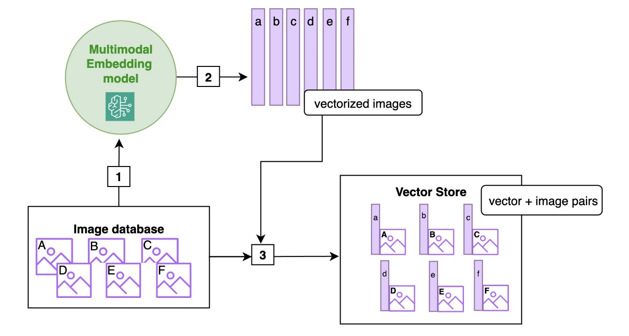

Originally appeared here:
From RAG to fabric: Lessons learned from building real-world RAGs at GenAIIC – Part 2
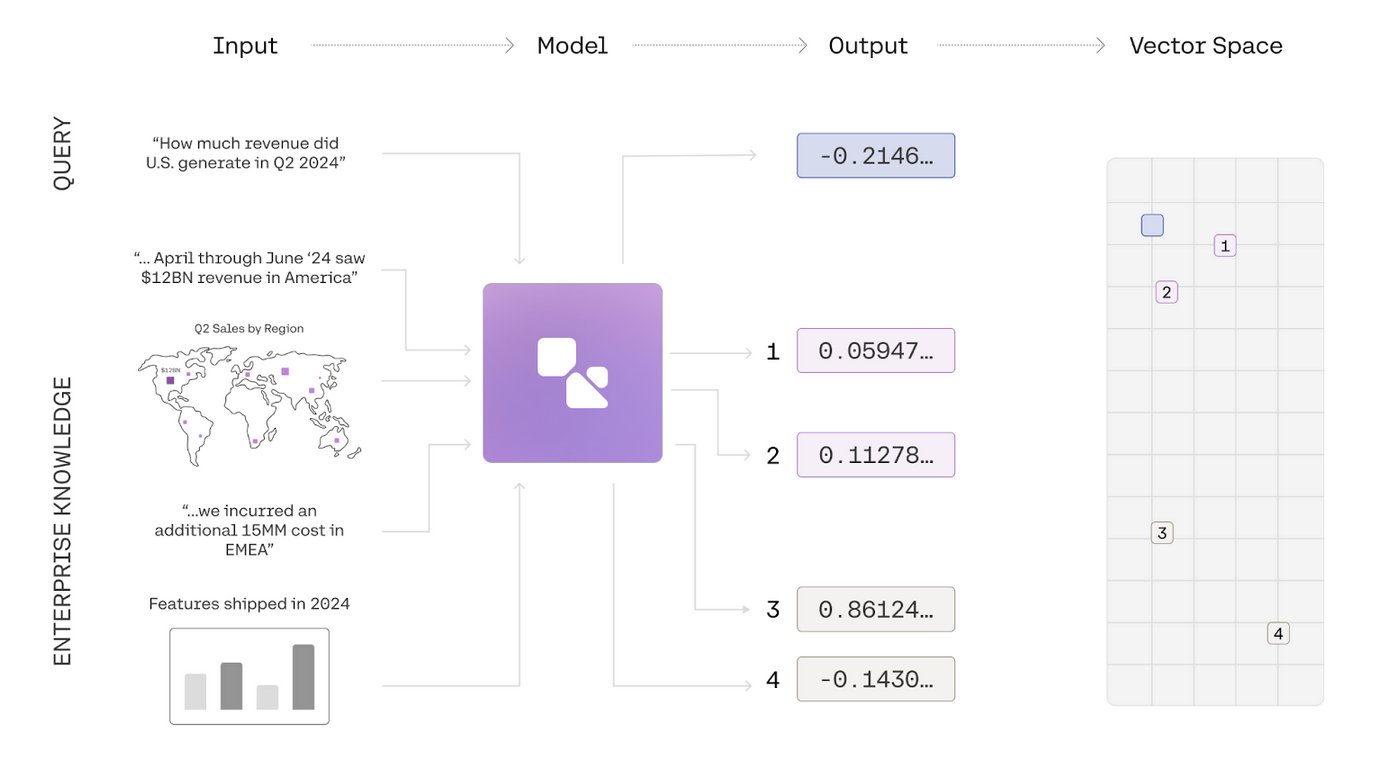

Originally appeared here:
Cohere Embed multimodal embeddings model is now available on Amazon SageMaker JumpStart