With the advent of generative AI, today’s foundation models (FMs), such as the large language models (LLMs) Claude 2 and Llama 2, can perform a range of generative tasks such as question answering, summarization, and content creation on text data. However, real-world data exists in multiple modalities, such as text, images, video, and audio. Take […]
pandas 2.2 was released on January 22nd 2024. Let’s take a look at the things this release introduces and how it will help us to improve our pandas workloads. It includes a bunch of improvements that will improve the user experience.
pandas 2.2 brought a few additional improvements that rely on the Apache Arrow ecosystem. Additionally, we added deprecations for changes that are necessary to make Copy-on-Write the default in pandas 3.0. Let’s dig into what this means for you. We will look at the most important changes in detail.
I am part of the pandas core team. I am an open source engineer for Coiled where I work on Dask, including improving the pandas integration.
Improved PyArrow support
We have introduced PyArrow backed DataFrame in pandas 2.0 and continued to improve the integration since then to enable a seamless integration into the pandas API. pandas has accessors for certain dtypes that enable specialized operations, like the string accessor, that provides many string methods. Historically, list and structs were represented as NumPy object dtype, which made working with them quite cumbersome. The Arrow dtype backend now enables tailored accessors for lists and structs, which makes working with these objects a lot easier.
This is a series that contains a dictionary in every row. Previously, this was only possible with NumPy object dtype and accessing elements from these rows required iterating over them. The struct accessor now enables direct access to certain attributes:
The next release will bring a CategoricalAccessor based on Arrow types.
Integrating the Apache ADBC Driver
Historically, pandas relied on SqlAlchemy to read data from an Sql database. This worked very reliably, but it was very slow. Alchemy reads the data row-wise, while pandas has a columnar layout, which makes reading and moving the data into a DataFrame slower than necessary.
The ADBC Driver from the Apache Arrow project enables users to read data in a columnar layout, which brings huge performance improvements. It reads the data and stores them into an Arrow table, which is used to convert to a pandas DataFrame. You can make this conversion zero-copy, if you set dtype_backend=”pyarrow” for read_sql.
Let’s look at an example:
import adbc_driver_postgresql.dbapi as pg_dbapi

df = pd.DataFrame(
   [
       [1, 2, 3],
       [4, 5, 6],
   ],
   columns=['a', 'b', 'c']
)
uri = "postgresql://postgres:postgres@localhost/postgres"
with pg_dbapi.connect(uri) as conn:
   df.to_sql("pandas_table", conn, index=False)

# for round-tripping
with pg_dbapi.connect(uri) as conn:
   df2 = pd.read_sql("pandas_table", conn)
The ADBC Driver currently supports Postgres and Sqlite. I would recommend everyone to switch over to this driver if you use Postgres, the driver is significantly faster and completely avoids round-tripping through Python objects, thus preserving the database types more reliably. This is the feature that I am personally most excited about.
Adding case_when to the pandas API
Coming from Sql to pandas, users often miss the case-when syntax that provides an easy and clean way to create new columns conditionally. pandas 2.2 adds a new case_when method, that is defined on a Series. It operates similarly to what Sql does.
The method takes a list of conditions that are evaluated sequentially. The new object is then created with those values in rows where the condition evaluates to True. The method should make it significantly easier for us to create conditional columns.
Copy-on-Write
Copy-on-Write was initially introduced in pandas 1.5.0. The mode will become the default behavior with 3.0, which is hopefully the next pandas release. This means that we have to get our code into a state where it is compliant with the Copy-on-Write rules. pandas 2.2 introduced deprecation warnings for operations that will change behavior.
df = pd.DataFrame({"x": [1, 2, 3]})

df["x"][df["x"] > 1] = 100
This will now raise a FutureWarning.
FutureWarning: ChainedAssignmentError: behaviour will change in pandas 3.0!
You are setting values through chained assignment. Currently this works in certain cases, but when
using Copy-on-Write (which will become the default behaviour in pandas 3.0) this will never work to
update the original DataFrame or Series, because the intermediate object on which we are setting
values will behave as a copy. A typical example is when you are setting values in a column of a
DataFrame, like:

df["col"][row_indexer] = value

Use `df.loc[row_indexer, "col"] = values` instead, to perform the assignment in a single step and
ensure this keeps updating the original `df`.
I wrote an earlier post that goes into more detail about how you can migrate your code and what to expect. There is an additional warning mode for Copy-on-Write that will raise warnings for all cases that change behavior:
pd.options.mode.copy_on_write = "warn"
Most of those warnings are only noise for the majority of pandas users, which is the reason why they are hidden behind an option.
This will raise a lengthy warning explaining what will change:
FutureWarning: Setting a value on a view: behaviour will change in pandas 3.0.
You are mutating a Series or DataFrame object, and currently this mutation will
also have effect on other Series or DataFrame objects that share data with this
object. In pandas 3.0 (with Copy-on-Write), updating one Series or DataFrame object
will never modify another.
The short summary of this is: Updating view will never update df, no matter what operation is used. This is most likely not relevant for most.
I would recommend enabling the mode and checking the warnings briefly, but not to pay too much attention to them if you are comfortable that you are not relying on updating two different objects at once.
This will give you the new release in your environment.
Conclusion
We’ve looked at a couple of improvements that will improve performance and user experience for certain aspects of pandas. The most exciting new features will come in pandas 3.0, where Copy-on-Write will be enabled by default.
Thank you for reading. Feel free to reach out to share your thoughts and feedback.
including 4 ways to make them and 2 ways to style them
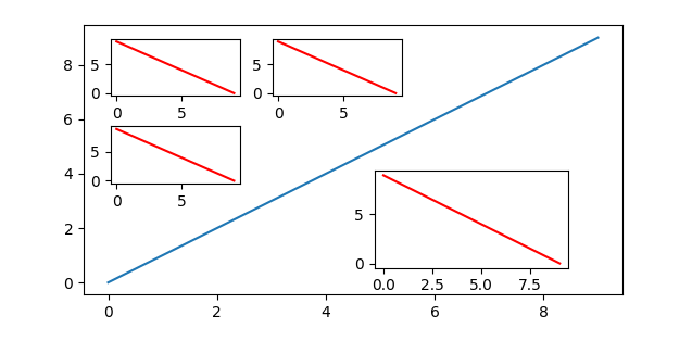
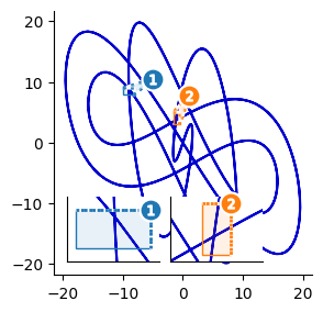
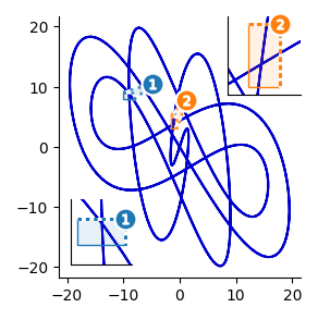
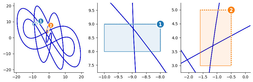
example plot with four inset axes
Inset axes are a powerful data visualization technique to highlight specific plot regions or add detailed subplots. They are a great way to make effective use of otherwise-emtpy figure space.
This tutorial shows 4 methods to create inset axes in matplotlib, which let you position insets relative to an axes, to an overall, figure, in absolute units (i.e., inches), or using a grid system — the latter useful in particular when working with multiple insets.
We’ll also cover 2 ways to style zoom insets: with classic leader lines and with color-coded overlays.
inset axes with color-coded overlays
At the end of this tutorial, you will be able to determine which approach best meets your needs —and have some code you can copy/paste to make it happen.
manual placement with axes-level coordinates: Axes.inset_axes, and
manual placement with figure-level coordinates: Figure.add_axes;
multi-inset auto-layout:Axes.inset_axes with outset.layout_corner_insets.
Adding zoom indicators:
5. leader lines: Axes.indicate_inset_zoom and
6. color-coded overlays: OutsetGrid.marqueeplot.
Sections 4 and 6 make use new tools from the open source outset library for multi-scale data visualization, which I recently released and am excited to share with the community.
Method 1: Using `mpl_toolkits.axes_grid1.inset_axes`
This function simplifies adding insets. Here’s how to use it, including an explanation of the `loc` parameter for positioning:
import matplotlib.pyplot as plt
from mpl_toolkits.axes_grid1.inset_locator import inset_axes

fig, ax = plt.subplots(); ax.set_box_aspect(0.5)  # main figure and axes
ax.plot([0, 9], [0, 9])  # example plot

# create inset axes & plot on them
inset_ax = inset_axes(ax, width="30%", height=1.2, loc="upper left")
inset_ax.plot([9, 0], [0, 9], color="r")
plt.xticks([]); plt.yticks([])  # strip ticks, which collide w/ main ax
Note that axes size can be specified relative to parent axes or in inches, as shown here with width and height, respectively.
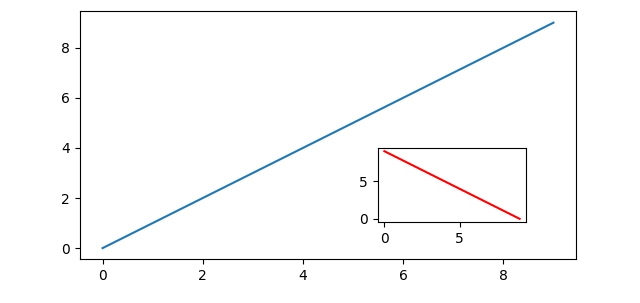
Matplotlib’s Axes class provides the inset_axes member function, which is a straightforward way to create insets relative to the parent axes:
import matplotlib.pyplot as plt

fig, ax = plt.subplots(); ax.set_box_aspect(0.5)  # main figure and axes
ax.plot([0, 9], [0, 9])  # example plot

# create inset axes & plot on them
ins_ax = ax.inset_axes([.6, .15, .3, .3])  # [x, y, width, height] w.r.t. ax
ins_ax.plot([9, 0], [0, 9], color="r")
Coordinates are specified relative to the parent axes, so — for example — (0, 0, 0.5, 0.2) will create an axes in the lower left-hand corner with width that takes up half of axes width and height that takes up 0.2 of axes height.
To position an inset relative to a parent axes ax in terms of inches, we must first calculate the size of the parent axes in inches.
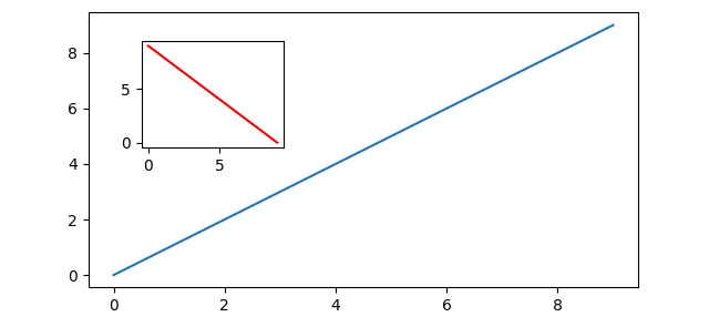
Matplotlib’s Figure class provides an analogous add_axes member function, which lets you position insets relative to the overall figure.
import matplotlib.pyplot as plt

fig, ax = plt.subplots(); ax.set_box_aspect(0.5)  # main figure and axes
ax.plot([0, 9], [0, 9])  # example plot

# create inset axes & plot on them
ins_ax = fig.add_axes([.2, .5, .2, .2])  # [x, y, width, height] w.r.t. fig
ins_ax.plot([9, 0], [0, 9], color="r")
Similarly to before, coordinates will be specified relative to the parent axes, so — for example — (0.5, 0.5, 0.3, 0.2) will create an axes 2/10ths the height of the overall figure and 3/10ths the width with the lower left corner centered within the figure.
Method 4: `Axes.inset_axes` with `outset.layout_corner_insets`
For this next example, we will use the outset library, which provides specialized tools for working with inset axes in matplotlib. It can be installed as python3 -m pip install outset.
The outset library provides the flexible outset.util.layout_corner_insets utility to position multiple inset axes within a specified corner of a main axes. Here’s how to use it to pick positions for calls to Axes.inset_axes.
import matplotlib.pyplot as plt
import outset

fig, ax = plt.subplots(); ax.set_box_aspect(0.5)  # main figure and axes
ax.plot([0, 9], [0, 9])  # example plot

# ------ pick inset axes positions: 3 in upper left, one in lower right
inset_positions = outset.util.layout_corner_insets(  # upper left positions
    3, "NW", # number insets and corner to position in
    # optional layout tweaks...
    inset_pad_ratio=(.2,.35), inset_grid_size=(.6,.65), inset_margin_size=.05)
inset_positions.append(  # generate lower right position & tack on to list
    outset.util.layout_corner_insets(1, "SE", inset_grid_size=.4))

# ----- create inset axes & plot on them
inset_axes = [*map(ax.inset_axes, inset_positions)]  # create inset axes
for iax in inset_axes:  # example plot
  iax.plot([9, 0], [0, 9], color="r")
Note the optional customizations to inset positioning made through keyword arguments to outset.util.layout_corner_insets. Here, “pad” refers to spacing between insets, “margin” refers to space between the insets and the main axes, and “grid size” refers to the overall fraction of axes space that insets are stacked into.
That covers it for techniques to place inset axes!
A common use case for inset axes is to provide magnification of an area of interest within the main plot. Next, we’ll look at two ways to visually correspond magnifying insets with a region of the main plot.
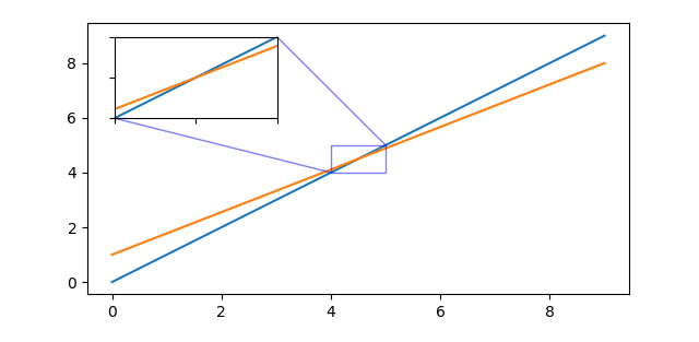
Method 5: Zoom Indicator Leaders
A classic approach depicting zoom relationships draws connecting lines between the corners of the inset axes and the region it is magnifying. This works especially well when plotting small numbers of insets.
Matplotlib’s Axes includes the indicate_inset_zoom member function for this purpose. Here’s how to use it.
from math import isclose; import matplotlib.pyplot as plt
# set up main fig/axes fig, main_ax = plt.subplots(); main_ax.set_box_aspect(0.5) inset_ax = main_ax.inset_axes( [0.05, 0.65, 0.3, 0.3], # [x, y, width, height] w.r.t. axes xlim=[4, 5], ylim=[4, 5], # sets viewport & tells relation to main axes xticklabels=[], yticklabels=[] )
# add plot content for ax in main_ax, inset_ax: ax.plot([0, 9], [0, 9]) # first example line ax.plot([0, 9], [1, 8]) # second example line
# careful! warn if aspect ratio of inset axes doesn't match main axes if not isclose(inset_ax._get_aspect_ratio(), main_ax._get_aspect_ratio()): print("chosen inset x/ylim & width/height skew aspect w.r.t. main axes!")
Note that to use Axes.indicate_inset_zoom, inset axes must be created using Axes.inset_axes.
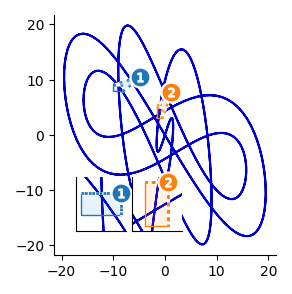
Method 6: Zoom Indicator Overlays
When working with larger numbers of insets, it may work better to correspond regions with numbered, color-coded highlights instead of leader lines.
The outset library’s OutsetGrid provides a marqueeplot member function for this purpose. Under this scheme, inset positioning is handled by outset.inset_outsets. Here’s how to create a zoom plot with color-coded position overlays.
from matplotlib import pyplot as plt
import numpy as np
import outset

# example adapted from https://matplotlib.org/stable/gallery/
i, a, b, c, d = np.arange(0.0, 2 * np.pi, 0.01), 1, 7, 3, 11

# 3 axes grid: source plot and two zoom frames
grid = outset.OutsetGrid([  # data coords for zoom sections...
     (-10, 8, -8, 9), (-1.6, 5, -0.5, 3)])  # ...as (x0, y0, x1, y1)
grid.broadcast(plt.plot,  # run plotter over all axes
    # subsequent kwargs go to the plotter
    np.sin(i * a) * np.cos(i * b) * 20,  # line coords
    np.sin(i * c) * np.cos(i * d) * 20,  # line coords
    c="mediumblue",  zorder=-1,  # line styling
)

# position insets over the source plot into lower/left ("SW") corner
outset.inset_outsets(grid, insets="SW")

grid.marqueeplot()  # render overlay annotations
Note that inset positioning can be more finely controlled via outset.util.layout_corner_insets, as used for Method 4 above:
...  # as before

customized_placements = outset.util.layout_corner_insets(
    2, "SW",  # 2 insets into the lower left corner
    inset_margin_size=0.05, inset_grid_size=(0.8, 0.55)  # layout params
)
outset.inset_outsets(grid, insets=customized_placements)
grid.marqueeplot()  # render overlay annotations
Inset placements can also be manually specified to outset.inset_outsetsusing axes-relative coordinates, too:
And, finally, to use bigger, side-by-side magnification panels instead of insets, just omit the call to outset.inset_outsets.
Conclusion
Inset axes are a great way to take your matplotlib visualizations to the next level, whether you’re looking to highlight specific data regions or add detailed subplots.
Here, we’ve covered the variety of approaches at your disposal, both built in to matplotlib and using the outset library. Each method offers unique advantages, ensuring a good fit for nearly any inset plotting scenario.
Now go make something informative and beautiful! Happy plotting 🙂
Further Information
matplotlib has some excellent inset example materials that are well worth checking out. In particular,
Formal argument-by-argument listings for all code covered here can be found in the API documentation pages for outset and matplotlib.
Both projects are open source on GitHub, matplotlib under a PSF license at matplotlib/matplotlib and outset under the MIT License at mmore500/outset — outset is a new project, consider leaving a ⭐️!
Joseph Early also has an excellent medium article on inset axes in matplotlib, which you can read here.
I currently serve as a postdoctoral scholar at the University of Michigan, where my work is supported by the Eric and Wendy Schmidt AI in Science Postdoctoral Fellowship, a Schmidt Futures program.
My appointment is split between the university’s Ecology and Evolutionary Biology Department, the Center for the Study of Complexity, and the Michigan Institute for Data Science.
disclosure: I am the author of the outset library.
Citations
J. D. Hunter, “Matplotlib: A 2D Graphics Environment”, Computing in Science & Engineering, vol. 9, no. 3, pp. 90–95, 2007. https://doi.org/10.1109/MCSE.2007.55
Using Poetry and Docker to Package Your Model for AWS Lambda
An accessible tutorial for one way to put a model into production, with special focus on troubleshooting and hiccups you might encounter along the way
I like to think of models as little critters. Photo by Jiawei Zhao on Unsplash
As promised, this week I’m coming with a more technical topic and taking a little break from all the discussions of business. I recently had an opportunity to deploy a new model using AWS Lambda, and I learned a few things when combining my usual development tooling (Poetry) with the infrastructure of Lambda. (Big hat tip to my teammate Aaron for teaching me new stuff!) I’m going to walk through the less obvious steps to getting a locally trained model deployed to Lambda successfully.
For my regular readers who are not interested in the nuts and bolts of model development, fear not, I’ll be back to commenting on social issues and machine learning next time!
Setting up your model architecture
If you don’t already have a preferred package manager/environment manager tool in Python, let me make a case for Poetry. It took me a while to get started and get the hang of it, but I’ve been using it for a couple of years now and have become a real fan. Some folks prefer venv or other more bare bones tooling, which is fine, but Poetry has some nice extra features that I think are worth it. (If you don’t have any experience with Poetry, please visit the official docs at https://python-poetry.org/ and they can get you set up.)
One of the selling points I’d like to emphasize is that Poetry makes it quite easy to package your project so that internal modules you create are callable without a lot of fuss. This means that you don’t have to fight the “Python says that module doesn’t exist” battle that I’m sure many of us are familiar with.
The example embedded here is just the head of the pyproject.toml file for a project like this one — notice the line starting with packages telling this env to include the package I’m creating in its imports. This is what lets me call things like from new_package.tools import stuff anywhere inside this project, even if those things are not in the immediate parent directory or whatever.
[tool.poetry] name = "new_package" version = "0.1.0" description = "What this package is gonna do" authors = [ "Stephanie Kirmer <[email protected]>", ]
packages = [{ include = "new_package"}] include = [{ path = "tests", format = "sdist" }]
Assuming you’re sold on Poetry, then you can use this to define your environment and manage all your dependencies, and you’ll be developing your model and its pipelines inside that project. Go ahead and build and train your model, and come back when that bit is done. I’ll wait.
Ok, welcome back! Because you know you’re going to be deploying this model through Docker in Lambda, that dictates how your inference pipeline should be structured.
You need to construct a “handler”. What is that, exactly? It’s just a function that accepts the JSON object that is passed to the Lambda, and it returns whatever your model’s results are, again in a JSON payload. So, everything your inference pipeline is going to do needs to be called inside this function.
In the case of my project, I’ve got a whole codebase of feature engineering functions: mountains of stuff involving semantic embeddings, a bunch of aggregations, regexes, and more. I’ve consolidated them into a FeatureEngineering class, which has a bunch of private methods but just one public one, feature_eng. So starting from the JSON that is being passed to the model, that method can run all the steps required to get the data from “raw” to “features”. I like setting up this way because it abstracts away a lot of complexity from the handler function itself. I can literally just call:
fe = FeatureEngineering(input=json_object)
processed_features = fe.feature_eng()
And I’m off to the races, my features come out clean and ready to go.
Be advised: I have written exhaustive unit tests on all the inner guts of this class because while it is neat to write it this way, I still need to be extremely conscious of any changes that might occur under the hood. Write your unit tests! If you make one small change, you may not be able to immediately tell you’ve broken something in the pipeline until it’s already causing problems.
The second half is the inference work, and this is a separate class in my case. I’ve gone for a very similar approach, which just takes in a few arguments.
The class initialization accepts the result of the feature engineering class’s method, so that handshake is clearly defined. Then the prediction method takes two items: the feature set (a JSON file listing all the feature names) and the model object, in my case a CatBoost classifier I’ve already trained and saved. I’m using the native CatBoost save method, but whatever you use and whatever model algorithm you use is fine. The point is that this method abstracts away a bunch of underlying stuff, and neatly returns the predictions object, which is what my Lambda is going to give you when it runs.
So, to recap, my “handler” function is essentially just this:
def lambda_handler(json_object, _context):
fe = FeatureEngineering(input=json_object) processed_features = fe.feature_eng()
Nothing more to it! You might want to add some controls for malformed inputs, so that if your Lambda gets an empty JSON, or a list, or some other weird stuff it’s ready, but that’s not required. Do make sure your output is in JSON or similar format, however (here I’m giving back a dict).
Building your Docker image
This is all great, we have a Poetry project with a fully defined environment and all the dependencies, as well as the ability to load the modules we create, etc. Good stuff. But now we need to translate that into a Docker image that we can put on AWS.
Here I’m showing you a skeleton of the dockerfile for this situation. First, we’re pulling from AWS to get the right base image for Lambda. Next, we need to set up the file structure that will be used inside the Docker image. This may or may not be exactly like what you’ve got in your Poetry project — mine is not, because I’ve got a bunch of extra junk here and there that isn’t necessary for the prod inference pipeline, including my training code. I just need to put the inference stuff in this image, that’s all.
The beginning of the dockerfile
FROM public.ecr.aws/lambda/python:3.9

ARG YOUR_ENV
ENV NLTK_DATA=/tmp
ENV HF_HOME=/tmp
In this project, anything you copy over is going to live in a /tmp folder, so if you have packages in your project that are going to try and save data at any point, you need to direct them to the right place.
You also need to make sure that Poetry gets installed right in your Docker image- that’s what will make all your carefully curated dependencies work right. Here I’m setting the version and telling pip to install Poetry before we go any further.
The next issue is making sure all the files and folders your project uses locally get added to this new image correctly — Docker copy will irritatingly flatten directories sometimes, so if you get this built and start seeing “module not found” issues, check to make sure that isn’t happening to you. Hint: add RUN ls -R to the dockerfile once it’s all copied to see what the directory is looking like. You’ll be able to view those logs in Docker and it might reveal any issues.
Also, make sure you copy everything you need! That includes the Lambda file, your Poetry files, your feature list file, and your model. All of this is going to be needed unless you store these elsewhere, like on S3, and make the Lambda download them on the fly. (That’s a perfectly reasonable strategy for developing something like this, but not what we’re doing today.)
We’re almost done! The last thing you should do is actually install your Poetry environment and then set up your handler to run. There are a couple of important flags here, including –no-dev , which tells Poetry not to add any developer tools you have in your environment, perhaps like pytest or black.
The end of the dockerfile
RUN poetry config virtualenvs.create false
RUN poetry install --no-dev

CMD [ "lambda_function.lambda_handler" ]
That’s it, you’ve got your dockerfile! Now it’s time to build it.
Make sure Docker is installed and running on your computer. This may take a second but it won’t be too difficult.
Go to the directory where your dockerfile is, which should be the the top level of your project, and run docker build . Let Docker do its thing and then when it’s completed the build, it will stop returning messages. You can see in the Docker application console if it’s built successfully.
Go back to the terminal and run docker image ls and you’ll see the new image you’ve just built, and it’ll have an ID number attached.
From the terminal once again, run docker run -p 9000:8080 IMAGE ID NUMBER with your ID number from step 3 filled in. Now your Docker image will start to run!
Open a new terminal (Docker is attached to your old window, just leave it there), and you can pass something to your Lambda, now running via Docker. I personally like to put my inputs into a JSON file, such as lambda_cases.json , and run them like so:
If the result at the terminal is the model’s predictions, then you’re ready to rock. If not, check out the errors and see what might be amiss. Odds are, you’ll have to debug a little and work out some kinks before this is all running smoothly, but that’s all part of the process.
Deploying to AWS and testing
The next stage will depend a lot on your organization’s setup, and I’m not a devops expert, so I’ll have to be a little bit vague. Our system uses the AWS Elastic Container Registry (ECR) to store the built Docker image and Lambda accesses it from there.
When you are fully satisfied with the Docker image from the previous step, you’ll need to build one more time, using the format below. The first flag indicates the platform you’re using for Lambda. (Put a pin in that, it’s going to come up again later.) The item after the -t flag is the path to where your AWS ECR images go- fill in your correct account number, region, and project name.
After this, you should authenticate to an Amazon ECR registry in your terminal, probably using the command aws ecr get-login-password and using the appropriate flags.
Finally, you can push your new Docker image up to ECR:
If you’ve authenticated correctly, this should only take a moment.
There’s one more step before you’re ready to go, and that is setting up the Lambda in the AWS UI. Go log in to your AWS account, and find the “Lambda” product.
This is what the header will look like, more or less.
Pop open the lefthand menu, and find “Functions”.
This is where you’ll go to find your specific project. If you have not set up a Lambda yet, hit “Create Function” and follow the instructions to create a new function based on your container image.
If you’ve already created a function, go find that one. From there, all you need to do is hit “Deploy New Image”. Regardless of whether it’s a whole new function or just a new image, make sure you select the platform that matches what you did in your Docker build! (Remember that pin?)
The last task, and the reason I’ve carried on explaining up to this stage, is to test your image in the actual Lambda environment. This can turn up bugs you didn’t encounter in your local tests! Flip to the Test tab and create a new test by inputting a JSON body that reflects what your model is going to be seeing in production. Run the test, and make sure your model does what is intended.
If it works, then you did it! You’ve deployed your model. Congratulations!
Troubleshooting
There are a number of possible hiccups that may show up here, however. But don’t panic, if you have an error! There are solutions.
If your Lambda runs out of memory, go to the Configurations tab and increase the memory.
If the image didn’t work because it’s too large (10GB is the max), go back to the Docker building stage and try to cut down the size of the contents. Don’t package up extremely large files if the model can do without them. At worst, you may need to save your model to S3 and have the function load it.
If you have trouble navigating AWS, you’re not the first. Consult with your IT or Devops team to get help. Don’t make a mistake that will cost your company lots of money!
If you have another issue not mentioned, please post a comment and I’ll do my best to advise.
Good luck, happy modeling!
Upcoming talks: I will be speaking remotely about data science career trajectories to the Overseas Chinese Association for Institutional Research (OCAIR) on Friday, April 12, at 1 pm US Central Time. Check with OCAIR about how to join if you’d like to tune in.
(All images in this post except the header photo are created by the author.)
We use cookies on our website to give you the most relevant experience by remembering your preferences and repeat visits. By clicking “Accept”, you consent to the use of ALL the cookies.
This website uses cookies to improve your experience while you navigate through the website. Out of these, the cookies that are categorized as necessary are stored on your browser as they are essential for the working of basic functionalities of the website. We also use third-party cookies that help us analyze and understand how you use this website. These cookies will be stored in your browser only with your consent. You also have the option to opt-out of these cookies. But opting out of some of these cookies may affect your browsing experience.
Necessary cookies are absolutely essential for the website to function properly. These cookies ensure basic functionalities and security features of the website, anonymously.
Cookie
Duration
Description
cookielawinfo-checkbox-analytics
11 months
This cookie is set by GDPR Cookie Consent plugin. The cookie is used to store the user consent for the cookies in the category "Analytics".
cookielawinfo-checkbox-functional
11 months
The cookie is set by GDPR cookie consent to record the user consent for the cookies in the category "Functional".
cookielawinfo-checkbox-necessary
11 months
This cookie is set by GDPR Cookie Consent plugin. The cookies is used to store the user consent for the cookies in the category "Necessary".
cookielawinfo-checkbox-others
11 months
This cookie is set by GDPR Cookie Consent plugin. The cookie is used to store the user consent for the cookies in the category "Other.
cookielawinfo-checkbox-performance
11 months
This cookie is set by GDPR Cookie Consent plugin. The cookie is used to store the user consent for the cookies in the category "Performance".
viewed_cookie_policy
11 months
The cookie is set by the GDPR Cookie Consent plugin and is used to store whether or not user has consented to the use of cookies. It does not store any personal data.
Functional cookies help to perform certain functionalities like sharing the content of the website on social media platforms, collect feedbacks, and other third-party features.
Performance cookies are used to understand and analyze the key performance indexes of the website which helps in delivering a better user experience for the visitors.
Analytical cookies are used to understand how visitors interact with the website. These cookies help provide information on metrics the number of visitors, bounce rate, traffic source, etc.
Advertisement cookies are used to provide visitors with relevant ads and marketing campaigns. These cookies track visitors across websites and collect information to provide customized ads.