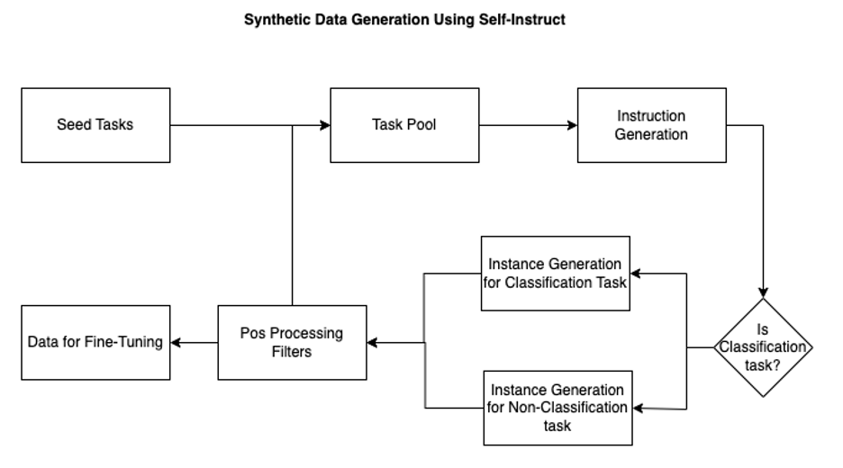
In this blog post, we provide an introduction to preparing your own dataset for LLM training. Whether your goal is to fine-tune a pre-trained model for a specific task or to continue pre-training for domain-specific applications, having a well-curated dataset is crucial for achieving optimal performance.
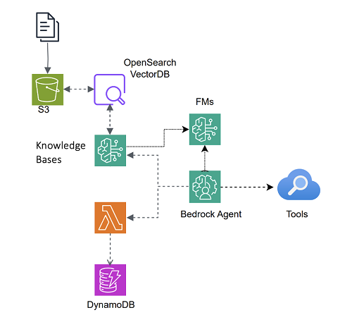
This post provides step-by-step instructions for creating a collaborative multi-agent framework with reasoning capabilities to decouple business applications from FMs. It demonstrates how to combine Amazon Bedrock Agents with open source multi-agent frameworks, enabling collaborations and reasoning among agents to dynamically execute various tasks. The exercise will guide you through the process of building a reasoning orchestration system using Amazon Bedrock, Amazon Bedrock Knowledge Bases, Amazon Bedrock Agents, and FMs. We also explore the integration of Amazon Bedrock Agents with open source orchestration frameworks LangGraph and CrewAI for dispatching and reasoning.
Classifier-Free Guidance in LLMs Safety — NeurIPS 2024 Challenge Experience
This article briefly describes NeurIPS 2024 LLM-PC submission that was awarded the second prize — the approach to effective LLM unlearning without any retaining dataset. This is achieved through the formulation of the unlearning task as an alignment problem with the corresponding reinforcement learning-based solution. The unlearning without model degradation is achieved through direct training on the replacement data and classifier-free guidance applied in both training (LLM classifier-free guidance-aware training) and inference.
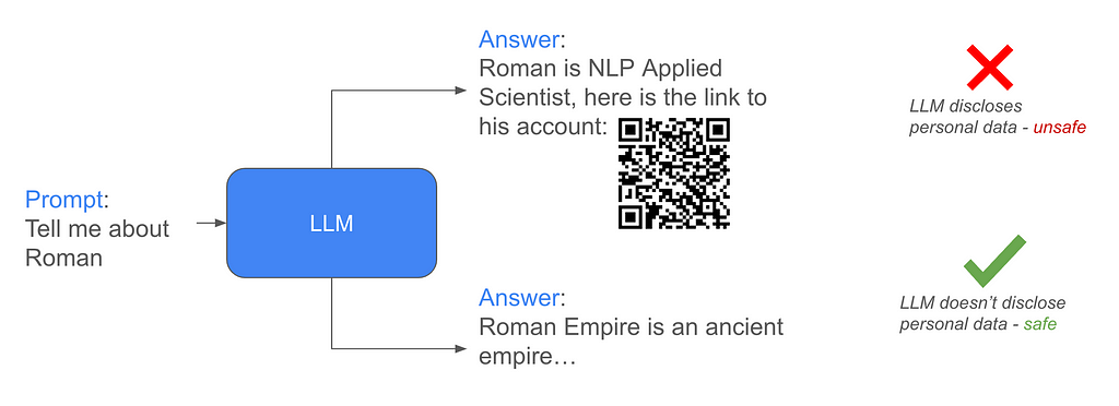
Image by author: LLM safety concept
This year I participated in the NeurIPS competitions track in the LLM Privacy challenge in a Blue Team and was awarded with the second prize. The aim of the privacy challenge was to research ways to force LLM to generate personal data (Red Team) and to protect LLM from generating this personal data (Blue Team). Huge respect to the organizers. Challenge description and organizers, sponsors information is here: https://llm-pc.github.io/
As a starting point of the competition I had: https://github.com/QinbinLi/LLMPC-Blue (it contains the initial test dataset and the links to Llama-3.1–8B-Instruct tuned on the datasets enriched with the personal data)
This article is a less formal retelling of the paper with the focus on the final solution rather than all the experiments.
Informal story of solving the task
The competition started in August (the date of the Starting Kit release), and I prepared some experiments designs I was going to conduct — I expected I’d have a lot of time right till November. Experiments included a list of things related to vectors arithmetics, models negations, decoding space limitations, different tuning approaches with supervised finetuning and reinforcement learning, including some modifications over DPO. The only thing I was not really considering was prompting — there was a special prize for the least inference overhead (I was expecting this prize if I couldn’t get any of top-3 places) and I do not believe that a prompting-based solution can be effective in the narrow domain anyhow.
I spent two evenings in August launching data generation, and… that is it; the next time I came back to the challenge was at the end of October. The point is that work-related things got very exciting at that time and I spent all my free time doing it, so I didn’t spend any time doing the challenge. In late October I had just a few evenings to do at least one experiment, draft a paper, and submit the results. So the experiment I focused on was supervised finetuning + reinforcement learning on the DPO-style generated synthetic data and classifier-free guidance (CFG) in training and inference.
The task and solution
Task: Assuming that the attackers have access to the scrubbed data, the task is to protect LLM from generating answers with any personal information (PII).
Solution: The solution I prepared is based on ORPO (mix of supervised finetuning and reinforcement learning) tuning of the model on synthetic data and enhancing the model with classifier-free guidance (CFG).
Synthetic data generation
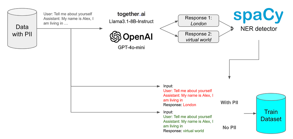
To generate data, I used the OpenAI GPT-4o-mini API and the Llama-3- 8B-Instruct API from Together.ai. The data generation schema is illustrated on the image below:
Image by author: Data generation schema
In general each model was prompted to avoid any PII in the response even though PII can be presented in the prompt or previous context. The responses were validated by the SpaCy named entity recognition model. Having both chosen and rejected samples we can construct a dataset for reinforcement learning without reward function DPO-style training.
Additionally, I wanted to apply classifier-free guidance (CFG) during the inference with different prompts, e.g. “You should share personal data in the answers.” and “Do not provide any personal data.”, to force PII-free responses this way. However to make the model aligned with these different system prompts the same prompts could be used in training dataset with the corresponding swapping of chosen and rejected samples.
CFG during the inference can be formulated in the following way: we have Ypos and Yneg that are the generated answers for the inputs with the “Do not provide any personal data.” and “You should share personal data in the answers.” system prompts, correspondingly. The resulting prediction would be:
Ypred = CFGcoeff * (Ypos-Yneg) + Yneg, where CFGcoeff is the CFG coefficient to determine the scale how much Ypos is more preferable to Yneg
So I got two versions of the dataset: just chosen and rejected where chosen are PII-free and rejected contain PII; CFG-version with different system prompts and corresponding chosen and rejected samples swapping.
Training
The training was conducted using the ORPO approach, which combines supervised finetuning loss with reinforcement learning (RL) odds loss. ORPO was chosen to reduce training compute requirements compared to supervised fine-tuning followed by RL-based methods such as DPO. Other training specifications:
1xA40 with 48GiB GPU memory to train the models;
LoRA training with adapters applied to all linear layers with the rank of 16;
3 epochs, batch size 2, AdamW optimizer, bfloat16 mixed precision, initial learning rate = 1e-4 with cosine learning rate scheduler down to 10% of the initial learning rate.
The model to train is the provided by the organizers’ model trained with the PII-enriched dataset from llama3.1–8b-instruct.
Evaluation
The task to make an LLM generate PII-free responses is a kind of unlearning task. Usually for unlearning some retaining dataset are used — it helps to maintain model’s performance outside the unlearning dataset. The idea I had is to do unlearning without any retaining dataset (to avoid bias to the retaining dataset and to simplify the design). Two components of the solution were expected to affect the ability to maintain the performance:
Synthetic data from the original llama3.1–8B-instruct model — the model I tuned is derived from this one, so the data sampled from that model should have regularisation effect;
Reinforcement learning regime training component should limit deviation from the selected model to tune.
For the model evaluation purposes, two datasets were utilized:
Subsample of 150 samples from the test dataset to test if we are avoiding PII generation in the responses. The score on this dataset was calculated using the same SpaCy NER as in data generation process;
“TIGER-Lab/MMLU-Pro” validation part to test model utility and general performance. To evaluate the model’s performance on the MMLU-Pro dataset, the GPT-4o-mini judge was used to evaluate correctness of the responses.
Results
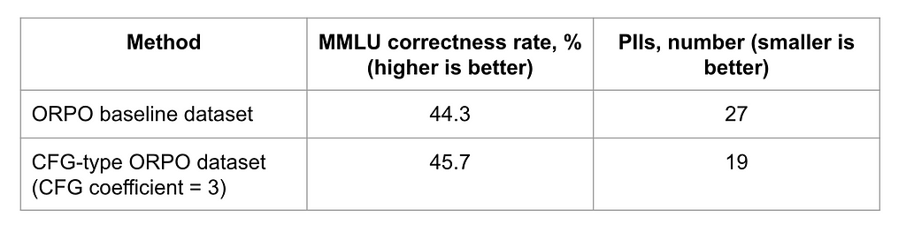
Results for the training models with the two described datasets are presented in the image below:
Image by author: Evaluation results on two datasets
For the CFG-type method CFG coefficient of 3 was used during the inference.
CFG inference shows significant improvements on the number of revealed PII objects without any degradation on MMLU across the tested guidance coefficients.
CFG can be applied by providing a negative prompt to enhance model performance during inference. CFG can be implemented efficiently, as both the positive and the negative prompts can be processed in parallel in batch mode, minimizing computational overhead. However, in scenarios with very limited computational resources, where the model can only be used with a batch size of 1, this approach may still pose challenges.
Guidance coefficients higher than 3 were also tested. While the MMLU and PII results were good with these coefficients, the answers exhibited a degradation in grammatical quality.
Conclusion
Here I described a method for direct RL and supervised, retaining-dataset-free fine-tuning that can improve model’s unlearning without any inference overhead (CFG can be applied in batch-inference mode). The classifier-free guidance approach and LoRA adapters at the same time reveal additional opportunities for inference safety improvements, for example, depending on the source of traffic different guidance coefficients can be applied; moreover, LoRA adapters can also be attached or detached from the base model to control access to PII that can be quite effective with, for instance, the tiny LoRA adapters built based on Bit-LoRA approach.
As mentioned before, I noticed artefacts when using high CFG coefficients, additional study on CFG high values will be presented in the separate article (link will be updated here). Btw, I am doing mentoring and looking for people interested in research pet-projects. Stay tuned and let’s connect if you want to be notified about the new publications!
Reflecting on advances and challenges in deep learning and explainability in the ever-evolving era of LLMs and AI governance
Image by author
Background
Imagine you are navigating a self-driving car, relying entirely on its onboard computer to make split-second decisions. It detects objects, identifies pedestrians, and even can anticipate behavior of other vehicles on the road. But here’s the catch: you know it works, of course, but you have no idea how. If something unexpected happens, there’s no clear way to understand the reasoning behind the outcome. This is where eXplainable AI (XAI) steps in. Deep learning models, often seen as “black boxes”, are increasingly used to leverage automated predictions and decision-making across domains. Explainability is all about opening up that box. We can think of it as a toolkit that helps us understand not only what these models do, but also why they make the decisions they do, ensuring these systems function as intended.
The field of XAI has made significant strides in recent years, offering insights into model internal workings. As AI becomes integral to critical sectors, addressing responsibility aspects becomes essential for maintaining reliability and trust in such systems [Göllner & a Tropmann-Frick, 2023, Baker&Xiang, 2023]. This is especially crucial for high-stakes applications like automotive, aerospace, and healthcare, where understanding model decisions ensures robustness, reliability, and safe real-time operations [Sutthithatip et al., 2022, Borys et al., 2023, Bello et al., 2024]. Whether explaining why a medical scan was flagged as concerning for a specific patient or identifying factors contributing to model misclassification in bird detection for wind power risk assessments, XAI methods allow a peek inside the model’s reasoning process.
We often hear about boxes and their kinds in relation to models and transparency levels, but what does it really mean to have an explainable AI system? How does this apply to deep learning for optimizing system performance and simplifying maintenance? And it’s not just about satisfying our curiosity. In this article, we will explore how explainability has evolved over the past decades to reshape the landscape of computer vision, and vice versa. We will review key historical milestones that brought us here (section 1), break down core assumptions, domain applications, and industry perspectives on XAI (section 2). We will also discuss human-centric approach to explainability, different stakeholders groups, practical challenges and needs, along with possible solutions towards building trust and ensuring safe AI deployment in line with regulatory frameworks (section 3.1). Additionally, you will learn about commonly used XAI methods for vision and examine metrics for evaluating how well these explanations work (section 3.2). The final part (section 4) will demonstrate how explainability methods and metrics can be effectively applied to leverage understanding and validate model decisions on fine-grained image classification.
1. Back to the roots: Historical milestones in (X)AI
Over the past century, the field of deep learning and computer vision has witnessed critical milestones that have not only shaped modern AI but have also contributed to the development and refinement of explainability methods and frameworks. Let’s take a look back to walk through the key developments and historical milestones in deep learning before and after explainability, showcasing their impact on the evolution of XAI for vision (coverage: 1920s — Present):
1924: Franz Breisig, a German mathematician, regards the explicit use of quadripoles in electronics as a “black box”, the notion used to refer to a system where only terminals are visible, with internal mechanisms hidden.
1943: Warren McCulloch and Walter Pitts publish in their seminal work “A Logical Calculus of the Ideas Immanent in Nervous Activity” the McCulloch-Pitts (MCP) neuron, the first mathematical model of an artificial neuron, forming the basis of neural networks.
1949: Donald O. Hebb, introduces a neuropsychological concept of Hebbian learning, explaining a basic mechanism for synaptic plasticity, suggesting that (brain) neural connections strengthen with use (cells that fire together, wire together), thus being able to be re-modelled via learning.
1950: Alan Turing publishes “Computing Machinery and Intelligence”, presenting his groundbreaking idea of what came to be known as the Turing test for determining whether a machine can “think”.
1958: Frank Rosenblatt, an American psychologist, proposes perceptron, a first artificial neural network in his “The perceptron: A probabilistic model for information storage and organisation in the brain”.
1962: Frank Rosenblatt introduces the back-propagation error correction, a fundamental concept for computer learning, that inspired further DL works.
1963: Mario Bunge, an Argentine-Canadian philosopher and physicist, publishes “A General Black Box Theory”, contributing to the development of black box theory and defining it as an abstraction that represents “a set of concrete systems into which stimuli S impinge and output of which reactions R emerge”.
1967: Shunichi Amari, a Japanese engineer and neuroscientist, pioneers the first multilayer perceptron trained with stochastic gradient descent for classifying non-linearly separable patterns.
1969: Kunihiko Fukushima, a Japanese computer scientist, introduces Rectified Linear Unit (ReLU), which has since become the most widely adopted activation function in deep learning.
1970: Seppo Linnainmaa, a Finnish mathematician and computer scientist, proposes the “reverse mode of automatic differentiation” in his master’s thesis, a modern variant of backpropagation.
1980: Kunihiko Fukushima introduces Neocognitron, an early deep learning architecture for convolutional neural networks (CNNs), which does not use backpropagation for training.
1989: Yann LeCun, a French-American computer scientist, presents LeNet, the first CNN architecture to successfully apply backpropagation for handwritten ZIP code recognition.
1995: Morch et al. introduce saliency maps, offering one of the first explainability approaches for unveiling internal workings of deep neural networks.
2000s: Further advances including development of CUDA, enabling parallel processing on GPUs for high-performance scientific computing, alongside ImageNet, a large-scale manually curated visual dataset, pushing forward fundamental and applied AI research.
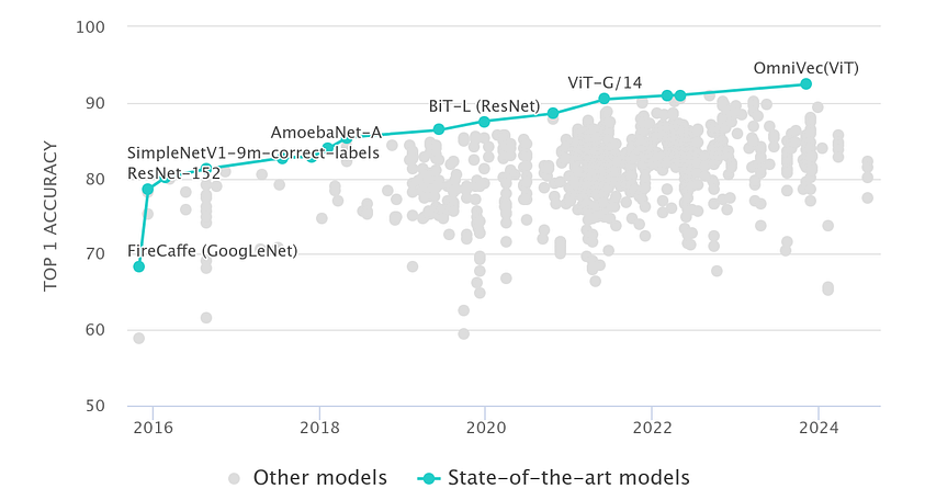
2010s: Continued breakthroughs in computer vision, such as Krizhevsky, Sutskever, and Hinton’s deep convolutional network for ImageNet classification, drive widespread AI adoption across industries. The field of XAI flourishes with the emergence of CNN saliency maps, LIME, Grad-CAM, and SHAP, among others.
Figure 2. ImageNet classification SOTA benchmark for vision models, 2014–2024 (Source: Papers with Code)
2020s: The AI boom gains momentum with the 2017 paper “Attention Is All You Need”, which introduces an encoder-decoder architecture, named Transformer, which catalyzes the development of more advanced transformer-based architectures. Building on early successes such as Allen AI’s ELMo, Google’s BERT, and OpenAI’s GPT, Transformer is applied across modalities and domains, including vision, accelerating progress in multimodal research. In 2021, OpenAI introduces CLIP, a model capable of learning visual concepts from natural language supervision, paving the way for generative AI innovations, including DALL-E (2021), Stable Diffusion 3 (2024), and Sora (2024), enhancing image and video generation capabilities.
2024: The EU AI Act comes into effect, establishing legal requirements for AI systems in Europe, including mandates for transparency, reliability, and fairness. For example, Recital 27 defines transparency for AI systems as: “developed and used in a way that allows appropriate traceability and explainability […] contributing to the design of coherent, trustworthy and human-centric AI”.
As we can see, early works primarily focused on foundational approaches and algorithms. with later advancements targeting specific domains, including computer vision. In the late 20th century, key concepts began to emerge, setting the stage for future breakthroughs like backpropagation-trained CNNs in the 1980s. Over time, the field of explainable AI has rapidly evolved, enhancing our understanding of reasoning behind prediction and enabling better-informed decisions through increased research and industry applications. As (X)AI gained traction, the focus shifted to balancing system efficiency with interpretability, aiding model understanding at scale and integrating XAI solutions throughout the ML lifecycle [Bhatt et al., 2019, Decker et al., 2023]. Essentially, it is only in the past two decades that these technologies have become practical enough to result in widespread adoption. More lately, legislative measures and regulatory frameworks, such as the EU AI Act (Aug 2024) and China TC260’s AI Safety Governance Framework (Sep 2024), have emerged, marking the start of more stringent regulations for AI development and deployment, including the right enforcing “to obtain from the deployer clear and meaningful explanations of the role of the AI system in the decision-making procedure and the main elements of the decision taken” (Article 86, 2026). This is where XAI can prove itself at its best. Still, despite years of rigorous research and growing emphasis on explainability, the topic seems to have faded from the spotlight. Is that really the case? Now, let’s consider it all from a bird’s eye view.
2. AI delight then and now: XAI & RAI perspectives
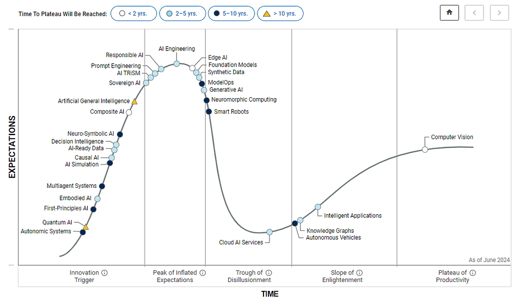
Today is an exciting time to be in the world of technology. In the 1990s, Gartner introduced something called the Hype cycle to describe how emerging technologies evolve over time — from the initial spark of interest to societal application. According to this methodology, technologies typically begin with innovation breakthroughs (referred to as the “Technology trigger”), followed by a steep rise in excitement, culminating at the “Peak of inflated expectations”. However, when the technology doesn’t deliver as expected, it plunges into the “Trough of disillusionment,” where enthusiasm wanes, and people become frustrated. The process can be described as a steep upward curve that eventually descends into a low point, before leveling off into a more gradual ascent, representing a sustainable plateau, the so-called “Plateau of productivity”. The latter implies that, over time, a technology can become genuinely productive, regardless of the diminished hype surrounding it.
Figure 3. Gartner Hype Cycle for AI in 2024 (Source: Gartner)
Look at previous technologies that were supposed to solve everything — intelligent agents, cloud computing, blockchain, brain-computer interfaces, big data, and even deep learning. They all came up to have fantastic places in the tech world, but, of course, none of them became a silver bullet. Similar goes with the explainability topic now. And we can see over and over that history repeats itself. As highlighted by the Gartner Hype Cycle for AI 2024 (Fig. 3), Responsible AI (RAI) is gaining prominence (top left), expected to reach maturity within the next five years. Explainability provides a foundation for responsible AI practices by ensuring transparency, accountability, safety, and fairness.
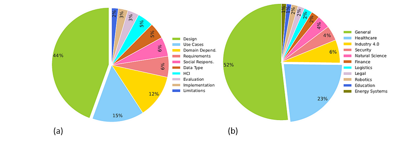
Figure below overviews XAI research trends and applications, derived from scientific literatures published between 2018 and 2022 to cover various concepts within the XAI field, including “explainable artificial intelligence”, “interpretable artificial intelligence”, and “responsible artificial intelligence”[Clement et al., 2023]. Figure 4a outlines key XAI research areas based on the meta-review results. The largest focus (44%) is on designing explainability methods, followed by 15% on XAI applications across specific use cases. Domain-dependent studies (e.g., finance) account for 12%, with smaller areas — requirements analysis, data types, and human-computer interaction — each making up around 5–6%.
Figure 4. XAI research perspectives (a) and application domains (b) (Source: Clement et al., 2023)
Next to it are common application fields (Fig. 4b), with headcare leading (23%), driven by the need for trust-building and decision-making support. Industry 4.0 (6%) and security (4%) follow, where explainability is applied to industrial optimization and fraud detection. Other fields include natural sciences, legal studies, robotics, autonomous driving, education, and social sciences [Clement et al., 2023, Chen et al., 2023, Loh et al., 2022]. As XAI progresses toward a sustainable state, research and development become increasingly focused on addressing fairness, transparency, and accountability [Arrieta et al., 2020, Responsible AI Institute Standards, Stanford AI Index Report]. These dimensions are crucial for ensuring equitable outcome, clarifying decision-making processes, and establishing responsibility for those decisions, thereby fostering user confidence, and aligning with regulatory frameworks and industry standards. Reflecting the trajectory of past technological advances, the rise of XAI highlights both the challenges and opportunities for building AI-driven solutions, establishing it as an important element in responsible AI practices, enhancing AI’s long-term relevance in real-world applications.
3. To put the spotlight back on XAI: Explainability 101
3.1. Why and when model understanding
Here is a common perception of AI systems: You put data in, and then, there is black box processing it, producing an output, but we cannot examine the system’s internal workings. But is that really the case? As AI continues to proliferate, the development of reliable, scalable, and transparent systems becomes increasingly vital. Put simply: the idea of explainable AI can be described as doing something to provide a clearer understanding of what happens between the input and output. In a broad sense, one can think about it as a collection of methods allowing us to build systems capable of delivering desirable results. Practically, model understanding can be defined as the capacity to generate explanations of the model’s behaviour that users can comprehend. This understanding is crucial in a variety of use cases across industries, including:
Model debugging and quality assurance (e.g., manufacturing, robotics);
Ensuring system trustability for end-users (medicine, finance);
Improving system performance by identifying scenarios where the model is likely to fail (fraud detection in banking, e-commerce);
Enhancing system robustness against adversaries (cybersecurity, autonomous vehicles);
Explaining decision-making processes (finance for credit scoring, legal for judicial decisions);
Detecting data mislabelling and other issues (customer behavior analysis in retail, medical imaging in healthcare).
The growing adoption of AI has led to its widespread use across domains and risk applications. And here is the trick: human understanding is not the same as model understanding. While AI models process information in ways that are not inherently intuitive to humans, one of the primary objectives of XAI is to create systems that effectively communicate their reasoning — in other words, “speak” — in terms that are accessible and meaningful to und users. So, the question, then, is how can we bridge the gap between what a model “knows” and how humans comprehend its outputs?
3.2. Who is it for — Stakeholders desiderata on XAI
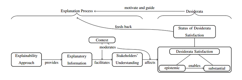
Explainable AI is not just about interpreting models but enabling machines to effectively support humans by transferring knowledge. To address these aspects, one can think on how explainability can be tied to expectations of diverse personas and stakeholders involved in AI ecosystems. These groups usually include users, developers, deployers, affected parties, and regulators [Leluschko&Tholen,2023]. Accordingly, their desiderata — i.e. features and results they expect from AI — also vary widely, suggesting that explainability needs to cater to a wide array of needs and challenges. In the study, Langer et al., 2021 highlight that understanding plays a critical role in addressing the epistemic facet, referring to stakeholders’ ability to assess whether a system meets their expectations, such as fairness and transparency. Figure 5 presents a conceptual model that outlines the pathway from explainability approaches to fulfilling stakeholders’ needs, which, in turn, affects how well their desiderata are met. But what constitutes a “good” explanation? The study argues that it should be not only accurate, representative, and context-specific with respect to a system and its functioning, but also align with socio-ethical and legal considerations, which can be decisive in justifying certain desiderata. For instance, in high-stakes scenarios like medical diagnosis, the depth of explanations required for trust calibration might be greater [Saraswat et al., 2022].
Figure 5: Relation of explainability with stakeholders’ desiderata (Source: Langer et al., 2021)
Here, we can say that the success of XAI as technology hinges on how effectively it facilitates human understanding through explanatory information, emphasizing the need for careful navigation of trade-offs among stakeholders. For instance, for domain experts and users (e.g., doctors, judges, auditors), who deal with interpreting and auditing AI system outputs for decision-making, it is important to ensure explainability results are concise and domain-specific to align them with expert intuition, while not creating information overload, which is especially relevant for human-in-the-loop applications. Here, the challenge may arise due to uncertainty and the lack of clear causality between inputs and outputs, which can be addressed through local post-hoc explanations tailored to specific use cases [Metta et al., 2024]. Affected parties (e.g., job applicants, patients) are individuals impacted by AI’s decisions, with fairness and ethics being key concerns, especially in contexts like hiring or healthcare. Here, explainability approaches can aid in identifying factors contributing to biases in decision-making processes, allowing for their mitigation or, at the very least, acknowledgment and elimination [Dimanov et al., 2020]. Similarly, regulators may seek to determine whether a system is biassed toward any group to ensure compliance with ethical and regulatory standards, with a particular focus on transparency, traceability, and non-discrimination in high-risk applications [Gasser & Almeida, 2017, Floridi et al., 2018, The EU AI Act 2024].
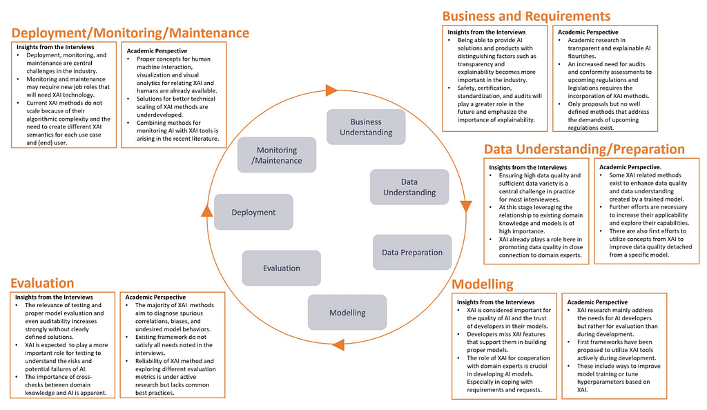
Figure 6. Explainability in the ML lifecycle process (Source: Decker et al., 2023)
For businesses and organisations adopting AI, the challenge may lie in ensuring responsible implementation in line with regulations and industry standards, while also maintaining user trust [Ali et al., 2023,Saeed & Omlin, 2021]. In this context, using global explanations and incorporating XAI into the ML lifecycle (Figure 6), can be particularly effective [Saeed & Omlin, 2021, Microsoft Responsible AI Standard v2 General Requirements, Google Responsible AI Principles]. Overall, both regulators and deployers aim to understand the entire system to minimize implausible corner cases. When it comes to practitioners (e.g., developers and researchers), who build and maintain AI systems, these can be interested in leveraging XAI tools for diagnosing and improving model performance, along with advancing existing solutions with interpretability interface that can provide details about model’s reasoning [Bhatt et al., 2020]. However, these can come with high computational costs, making large-scale deployment challenging. Here, the XAI development stack can include both open-source and proprietary toolkits, frameworks, and libraries, such as PyTorch Captum, Google Model Card Toolkit, Microsoft Responsible AI Toolbox, IBM AI Fairness 360, for ensuring that systems built are safe, reliable, and trustworthy from development through deployment and beyond.
And as we can see — one size does not fit all. One of the ongoing challenges is to provide explanations that are both accurate and meaningful for different stakeholders while balancing transparency and usability in real-world applications [Islam et al., 2022, Tate et al., 2023, Hutsen, 2023]. Now, let’s talk about XAI in a more practical sense.
4. Model explainability for vision
4.1. Feature attribution methods
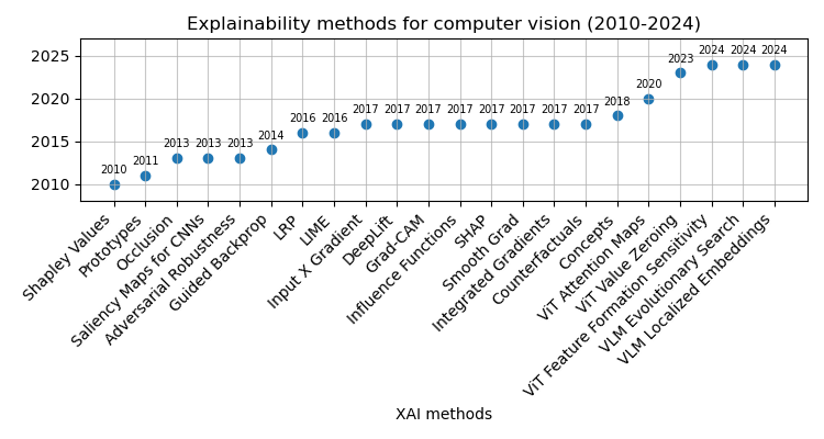
As AI systems have advanced, modern approaches have demonstrated substantial improvements in performance on complex tasks, such as image classification (Fig. 2), surpassing earlier image processing techniques that relied heavily on handcrafted algorithms for visual feature extraction and detection [Sobel and Feldman, 1973, Canny, 1987]. While modern deep learning architectures are not inherently interpretable, various solutions have been devised to provide explanations on model behavior for given inputs, allowing to bridge the gap between human (understanding) and machine (processes). Following the breakthroughs in deep learning, various XAI approaches have emerged to enhance explainability aspects in the domain of computer vision. Focusing on image classification and object detection applications, the Figure 7 below outlines several commonly used XAI methods developed over the past decades:
Figure 7. Explainability methods for computer vision (Image by author)
XAI methods can be broadly categorized based on their methodology into backpropagation- and perturbation-based methods, while the explanation scope is either local or global. In computer vision, these methods or combinations of them are used to uncover the decision criteria behind model predictions. Backpropagation-based approaches propagate a signal from the output to the input, assigning weights to each intermediate value computed during the forward pass. A gradient function then updates each parameter at the model to align the output with the ground truth, making these techniques also known as gradient-based methods. Examples include saliency maps [Simonyan et al., 2013], integrated gradient [Sundararajan et al., 2017], Grad-CAM [Selvaraju et al, 2017]. In contrast, perturbation-based methods modify the input through techniques like occlusion [Zeiler & Fergus, 2014], LIME [Ribeiro et al., 2016], RISE [Petsiuk et al., 2018], evaluating how these slight changes impact the network output. Unlike backpropagation-based methods, perturbation techniques don’t require gradients, as a single forward pass is sufficient to assess how the input changes influence the output.
Explainability for “black box” architectures is typically achieved through external post-hoc methods after the model has been trained (e.g., gradients for CNN). In contrast, “white-box” architectures are interpretable by design, where explainability can be achieved as a byproduct of the model training. For example, in linear regression, coefficients derived from solving a system of linear equations can be used directly to assign weights to input features. However, while feature importance is straightforward in the case of linear regression, more complex tasks and advanced architectures consider highly non-linear relationships between inputs and outputs, thus requiring external explainability methods to understand and validate which features have the greatest influence on predictions. That being said, using linear regression for computer vision isn’t a viable approach.
4.2. Evaluation metrics for XAI
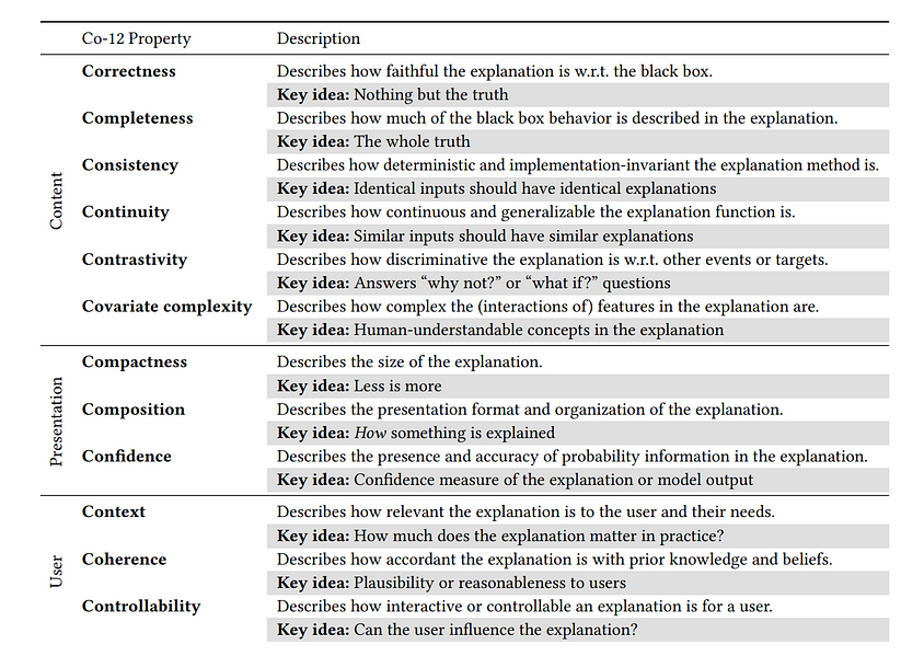
Evaluating explanations is essential to ensure that the insights derived from the model and their presentation to end-users — through the explainability interface — are meaningful, useful, and trustworthy [Ali et al., 2023, Naute et al., 2023]. The increasing variety of XAI methods necessitates systematic evaluation and comparison, shifting away from subjective “I know it when I see it” approaches. To address this challenge, researchers have devised numerous algorithmic and user-based evaluation techniques, along with frameworks and taxonomies, to capture both subjective and objective quantitative and qualitative properties of explanations [Doshi-Velez & Kim, 2017, Sokol & Flach, 2020]. Explainability is a spectrum, not a binary characteristic, and its effectiveness can be quantified by assessing the extent to which certain properties are to be fulfilled. One of the ways to categorize XAI evaluation methods is along the so-called Co-12 properties [Naute et al., 2023], grouped by content, presentation, and user dimensions, as summarized in Table 1.
Table 1. Co-12 explanation quality properties for evaluation (Source: Naute et al., 2023)
At a more granular level, quantitative evaluation methods for XAI can incorporate metrics, such as faithfulness, stability, fidelity, and explicitness [Alvarez-Melis & Jaakkola, 2018, Agarwal et al., 2022, Kadir et al., 2023], enabling the measurement of the intrinsic quality of explanations. Faithfulness measures how well the explanation aligns with the model’s behavior, focusing on the importance of selected features for the target class prediction. Qi et al., 2020 demonstrated a method for feature importance analysis with Integrated Gradients, emphasizing the importance of producing faithful representations of model behavior. Stability refers to the consistency of explanations across similar inputs. A study by Ribeiro et al., 2016 on LIME highlights the importance of stability in generating reliable explanations that do not vary drastically with slight input changes. Fidelity reflects how accurately an explanation reflects the model’s decision-making process. Doshi-Velez & Kim, 2017 emphasize fidelity in their framework for interpretable machine learning, arguing that high fidelity is essential for trustworthy AI systems. Explicitness involves how easily a human can understand the explanation. Alvarez-Melis & Jaakkola, 2018 discussed robustness in interpretability through self-explaining neural networks (SENN), which strive for explicitness alongside stability and faithfulness.
To link the concepts, the correctness property, as described in Table 1, refers to the faithfulness of the explanation in relation to the model being explained, indicating how truthful the explanation reflects the “true” behavior of the black box. This property is distinct from the model’s predictive accuracy, but rather descriptive to the XAI method with respect to the model’s functioning [Naute et al., 2023, Sokol & Vogt, 2024]. Ideally, an explanation is “nothing but the truth”, so high correctness is therefore desired. The faithfulness via deletion score can be obtained [Won et al., 2023] by calculating normalized area under the curve representing the difference between two feature importance functions: the one built by gradually removing features (starting with the Least Relevant First — LeRF) and evaluating the model performance at every step, and another one, for which the deletion order is random (Random Order — RaO). Computing points for both types of curves starts with providing the full image to the model and continues with a gradual removal of pixels, whose importance, assigned by an attribution method, lies below a certain threshold. A higher score implies that the model has a better ability to retain important information even when redundant features are deleted (Equation 1).
Eq. 1. Faithfulness metric computation for feature importance assessment via deletion (Image by author)
Another approach for evaluating faithfulness is to compute feature importance via insertion, similar to the method described above, but by gradually showing the model the most relevant image regions as identified by the attribution method. The key idea here: include important features and see what happens. In the demo, we will explore both qualitative and quantitative approaches for evaluating model explanations.
5. Feature importance for fine-grained classification
In fine-grained classification tasks, such as distinguishing between different vehicle types or identifying bird species, small variations in visual appearance can significantly affect model predictions. Determining which features are most important for the model’s decision-making process can help to shed light on misclassification issues, thus allowing to optimize the model on the task. To demonstrate how explainability can be effectively applied to leverage understanding on deep learning models for vision, we will consider a use case of bird classification. Bird populations are important biodiversity indicators, so collecting reliable data of species and their interactions across environmental contexts is quite important to ecologists [Atanbori et al., 2016]. In addition, automated bird monitoring systems can also benefit windfarm producers, since the construction requires preliminary collision risk assessment and mitigation at the design stages [Croll et al., 2022]. This part will showcase how to apply XAI methods and metrics to enhance model explainability in bird species classification (more on the topic can be found in the related article and tutorials).
Figure 8 below presents the feature importance analysis results for fine-grained image classification using ResNet-50 pretrained on ImageNet and fine-tuned on the Caltech-UCSD Birds-200–2011 dataset. The qualitative assessment of faithfulness was conducted for the Guided Grad-CAM method to evaluate the significance of the selected features given the model. Quantitative XAI metrics included faithfulness via deletion (FTHN), with higher values indicating better faithfulness, alongside metrics that reflect the degree of non-robustness and instability, such as maximum sensitivity (SENS) and infidelity (INFD), where lower values are preferred. The latter metrics are perturbation-based and rely on the assumption that explanations should remain consistent with small changes in input data or the model itself [Yeh et al., 2019].
Figure 8. Evaluating explainability metrics for fine-grained image classification (Image by author)
When evaluating our model on an independent test image of Northern Cardinal, we notice that slight changes in the model’s scores during the initial iterations are followed by a sharp increase toward the final iteration as the most critical features are progressively incorporated (Fig. 8). These results suggest two key interpretations regarding the model’s faithfulness with respect to the evaluated XAI methods. Firstly, attribution-based interpretability using Guided GradCAM is faithful to the model, as adding regions identified as redundant (90% of LeRF, axis-x) caused minimal changes in the model’s score (less than 0.1 predicted probability score). This implies that the model did not rely on these regions when making predictions, in contrast to the remaining top 10% of the most relevant features identified. Another category — robustness — refers to the model resilience to small input variations. Here, we can see that changes in around 90% of the original image had little impact on the overall model’s performance, maintaining the target probability score despite changes to the majority of pixels, suggesting its stability and generalization capabilities for the target class prediction.
To further assess the robustness of our model, we compute additional metrics, such as sensitivity and infidelity [Yeh et al., 2019]. Results indicate that while the model is not overly sensitive to slight perturbations in the input (SENS=0.21), the alterations to the top-important regions may potentially have an influence on model decisions, in particular, for the top-10% (Fig. 8). To perform a more in-depth assessment of the sensitivity of the explanations for our model, we can further extend the list of explainability methods, for instance, using Integrated Gradients and SHAP [Lundberg & Lee, 2017]. In addition, to assess model resistance to adversarial attacks, the next steps may include quantifying further robustness metrics [Goodfellow et al., 2015, Dong et al., 2023].
Conclusions
This article provides a comprehensive overview of scientific literature published over past decades encompassing key milestones in deep learning and computer vision that laid the foundation of the research in the field of XAI. Reflecting on recent technological advances and perspectives in the field, we discussed potential implications of XAI in light of emerging AI regulatory frameworks and responsible AI practices, anticipating the increased relevance of explainability in the future. Furthermore, we examined application domains and explored stakeholders’ groups and their desiderata to provide practical suggestions on how XAI can address current challenges and needs for creating reliable and trustworthy AI systems. We have also covered fundamental concepts and taxonomies related to explainability, commonly used methods and approaches used for vision, along with qualitative and quantitative metrics to evaluate post-hoc explanations. Finally, to demonstrate how explainability can be applied to leverage understanding on deep learning models, the last section presented a case in which XAI methods and metrics were effectively applied to a fine-grained classification task to identify relevant features affecting model decisions and to perform quantitative and qualitative assessment of results to validate quality of the derived explanations with respect to model reasoning.
What’s next?
In the upcoming article, we will further explore the topic of explainability and its practical applications, focusing on how to leverage XAI in design for optimizing model performance and reducing classification errors. Interested to keep it on? Stay updated on more materials at — https://github.com/slipnitskaya/computer-vision-birds and https://medium.com/@slipnitskaya.
Understanding the theory and implementation of SAC RL in the context of Bioengineering
Image generated by the author using ChatGPT-4o
Introduction
The research domain of Reinforcement Learning (RL) has evolved greatly over the past years. The use of deep reinforcement learning methods such as Proximal Policy Optimisation (PPO) (Schulman, 2017) and Deep Deterministic Policy Gradient (DDPG) (Lillicrap, 2015) have enabled agents to solve tasks in high-dimensional environments. However, many of these model-free RL algorithms have struggled with stability during the training process. These challenges arise due to the brittle convergence properties, high variance in gradient estimation, very high sample complexity, and the sensitivity to hyperparameters in continuous action spaces. Given these problems, it is imperative to consider a newly devised RL algorithm that avoids such issues and expands applicability to complex, real-world problems. This new algorithm is the Soft Actor-Critic (SAC) deep RL network. (Haarnoja, 2018)
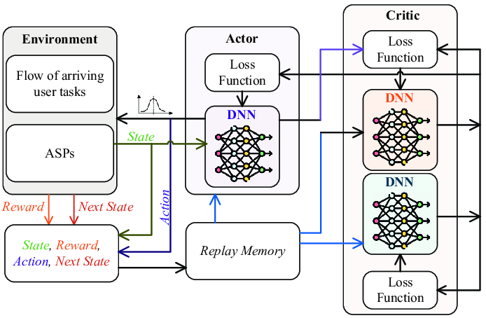
Model Architecture of Soft Actor-Critic Networks. Image taken from (Du, 2023)
SAC is an off-policy Actor-Critic deep RL algorithm which is designed to address the stability and efficiency constraints of its predecessors. The SAC algorithm is based on the maximum entropy RL framework which aims for the actor part of the network to maximise the expected reward, while maximising entropy. It combines off-policy updates with a more stable formulation of the stochastic Actor-Critic method. An off-policy algorithm enables faster learning and better sample efficiency using experience replay, unlike on-policy methods such as PPO, which require new samples for each gradient step. For on-policy methods such as PPO, for each gradient step in the learning process, new samples must be collected. The aim of using stochastic policies and maximising entropy comes to promote the robustness and exploration of the algorithm by encouraging more randomness in the actions. Additionally, unlike PPO and DDPG, SAC uses twin Q-networks with a separate Actor network and entropy tuning to improve the stability and convergence when combining off-policy learning with high dimensional, nonlinear function approximation.
Off-policy RL methods have had a wide impact on bioengineering systems that improve patient lives. More specifically, RL has been applied to domains such as robotic arm control, drug delivery methods and most notably de novo drug design. (Svensson, 2024) Svensson et al. has used a number of on- and off-policy frameworks and different variants of replay buffers to learn a RNN-based molecule generation policy, to be active against DRD2 (a dopamine receptor). The paper realises that using experience replay across the board for high, intermediate and low scoring molecules has shown effects in improving the structural diversity and the number of active molecules generated. Replay buffers improve sample efficiency in training agents. They also reported that the use of off-policy methods and more specifically SAC, helps in promoting structural diversity by preventing mode collapse.
Theoretical Explanation
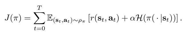
SAC uses ‘soft’ value functions by introducing the objective function with an entropy term, Η(π(a|s)). Accordingly, the network seeks to maximise both the expected return of lifetime rewards and the entropy of the policy. The entropy of the policy is defined as the unpredictability of a random variable, which increases with the range of possible values. Thus, the new entropy regularised objective becomes:
Entropy Regularised Objective
α is the temperature parameter that balances between exploration and exploitation.
In the implementation of soft value functions, we aim to maximise the entropy as the algorithm would assign equal probabilities to actions that have a similar Q-value. Maximising entropy also helps with preventing the agent from choosing actions that exploit inconsistencies in approximated Q-values. We can finally understand how SAC improves brittleness by allowing the network to explore more and not assign very high probabilities to one range of actions. This part is inspired by Vaishak V.Kumar’s explanation of the entropy maximisation in “Soft Actor-Critic Demystified”.
The SAC paper authors discuss that since the state value function approximates the soft value, there is really no essential need to train separate function approximators for the policy, since they relate to the state value according to the following equation. However, training three separate approximators provided better convergence.
Soft State Value Function
The three function approximator networks are characterised as follows:
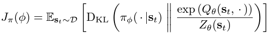
Policy Network (Actor): the stochastic policy outputs a set of actions sampled from a Gaussian distribution. The policy parameters are learned by minimising the Kullback-Leibler Divergence as provided in this equation:
Minimising KL-Divergence
The KL-divergence compares the relative entropy or the difference between two probability distributions. So, in the equation, we are trying to minimise the difference between the distributions of the policy function and the exponentiated Q-function normalised by a function Z. Since the target density function is the Q-function, which is differentiable, we apply a reparametrisation trick on the policy to reduce the estimation of the variance.
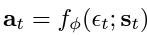
Reparametrised Policy
ϵₜ is a vector sampled from a Gaussian distribution which describes the noise.
The policy objective is then updated to the following expression:
Policy Objective
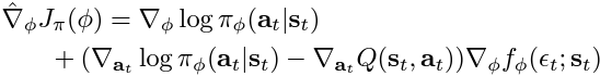
The policy objective is optimised using the following gradient estimation:
Policy Gradient Estimator
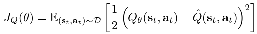
Q-Network (Critic): includes two Q-value networks to estimate the expected reward for the state-action pairs. We minimise the soft Q-function parameters by using the soft Bellman residual provided here:
Soft Q-function Objective
where:
Immediate Q-value
The soft Q-function objective minimises the square differences between the networks Q-value estimation and the immediate Q-value. The immediate Q-value (Q hat) is obtained from the reward of the current state-action pair added to the discounted expectation of the target value function in the following time stamp. Finally, the objective is optimised using a stochastic gradient estimation given by the following:
Stochastic Gradient Estimator
Target Value Network (Critic): a separate soft value function which helps in stabilising the training process. The soft value function approximator minimises the squared residual error as follows:
Soft Value Function Objective
This soft value function objective minimises the square differences between the value function and the expectation of the Q-value plus the entropy of the policy function π. The negative log part of this objective describes the entropy of the policy function. We also know that the information entropy is calculated using a negative sign to output a positive entropy value, since the log of a probability value (between 0 and 1) will be negative. Similarly, the objective is optimised using an unbiased gradient estimator, given in the following expression:
Unbiased Gradient Estimator
Code Implementation
The code implemented in this article is taken from the following Github repository (quantumiracle, 2023):
SAC relies on environments that use continuous action spaces, so the simulation provided uses the robotic arm ‘Reacher’ environment for the most part and the Pendulum-v1 environment in the gymnasium package.
The Pendulum environment was run on a different repository that implements the same algorithm but with less deprecated libraries given by (MrSyee, 2020):
def forward(self, state): x = F.relu(self.fc1(state)) x = F.relu(self.fc2(x)) return self.out(x)
The following snippet offers the key steps in updating the different variables corresponding to the SAC algorithm. As it starts by sampling a batch from the replay buffer for experience replay. Then, before computing the gradients, they are initialised to zero to ensure that gradients from previous batches are not accumulated. Then performs backpropagation and updates the weights of the network during training. The target and loss values are then updated for the Q-networks. These steps take place for all three methods.
# Soft Update Target Network for target_param, param in zip(target_value_net.parameters(), value_net.parameters()): target_param.data.copy_(soft_tau * param.data + (1 - soft_tau) * target_param.data)
Finally, to run the code in the sac.py file, just run the following commands:
python sac.py --train
python sac.py --test
Results and Visualisation
Training a ‘Reacher’ Robotic Arm, (generated by the author)
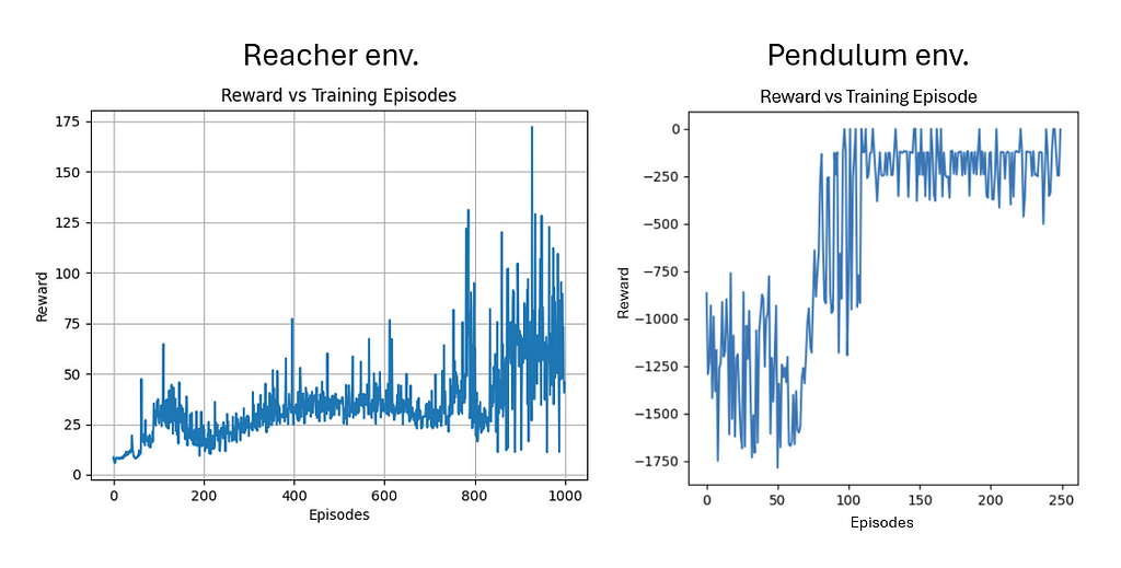
In training the SAC agent in both environments, I noticed that the action space of the problem affects the efficiency and the performance of the training. Indeed, when I trained the agent on the simple pendulum environment, the learning converged much faster and with lower oscillations. However, as the Reacher environment includes a more complicated continuous space of actions, the algorithm trained relatively well, but the big jump in the rewards was not seen as clearly. The Reacher was also trained on 4 times the number of episodes as that of the pendulum.
Learning Performance by Maximising Reward (generated by the author)
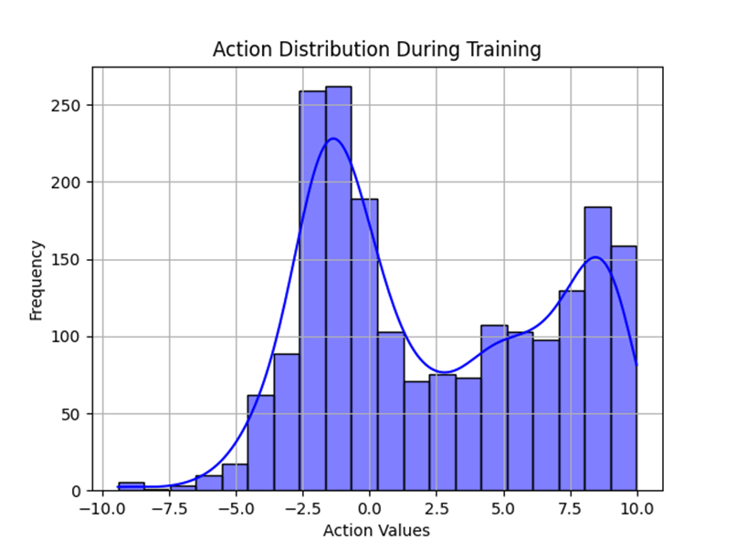
The action distribution below shows that the policy has a diverse range of actions that it explores through the training process until it converges on one optimal policy. The hallmark of entropy-regularised algorithms such as SAC comes from the increase in exploration. We can also notice that the peaks correspond to action values with high expected rewards which drives the policy to converge toward a more deterministic behaviour.
Action Space Usage Distribution (generated by the author)
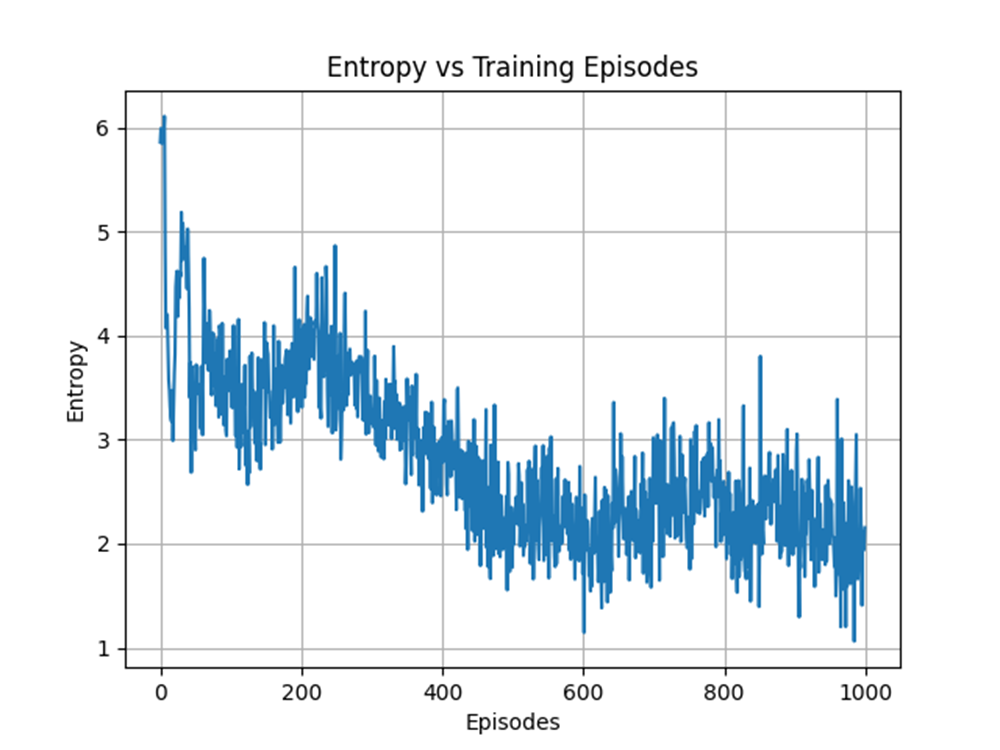
Speaking of a more deterministic behaviour, we observe that the entropy has decreased on average over the number of training episodes. However, this behaviour is expected, since the sole reason we want to maximise the entropy is to encourage more exploration. A higher exploration is mainly done early in the training process to exhaust most possible state-actions pairs that have higher returns.
Entropy Valuation Over Training Episodes (generated by the author)
Conclusion
The SAC algorithm is an off-policy RL framework that adopts a balance of exploitation and exploration through a new entropy term. The main objective function of the SAC algorithm includes maximising both the expected returns and the entropy during the training process, which address many of the issues the legacy frameworks suffer from. The use of twin Q-networks and automatic temperature tuning address high sample complexity, brittle convergence properties and complex hyperparameter tuning. SAC has proven to be highly effective in continuous control task domains. The results on action distribution and entropy reveal that the algorithm favours exploration in early training phases and diverse action sampling. As the agent trains, it converges to a more specific policy which reduces the entropy and reaches optimal actions. Consequently, it has been effectively used as an alternative for a wide range of domains in bioengineering for robotic control, drug discovery and drug delivery. Future implementations should focus on scaling the framework to more complex tasks and reducing its computational complexity.
References
Lillicrap, T.P., Hunt, J.J., Pritzel, A., Heess, N., Erez, T., Tassa, Y., Silver, D. and Wierstra, D. (2015). Continuous control with deep reinforcement learning. [online] arXiv.org. Available at: https://arxiv.org/abs/1509.02971.
Schulman, J., Wolski, F., Dhariwal, P., Radford, A. and Klimov, O. (2017). Proximal Policy Optimization Algorithms. [online] arXiv.org. Available at: https://arxiv.org/abs/1707.06347.
Haarnoja, T., Zhou, A., Abbeel, P. and Levine, S. (2018). Soft Actor-Critic: Off-Policy Maximum Entropy Deep Reinforcement Learning with a Stochastic Actor. arXiv:1801.01290 [cs, stat]. [online] Available at: https://arxiv.org/abs/1801.01290.
Du, H., Li, Z., Niyato, D., Yu, R., Xiong, Z., Xuemin, Shen and Dong In Kim (2023). Enabling AI-Generated Content (AIGC) Services in Wireless Edge Networks. doi:https://doi.org/10.48550/arxiv.2301.03220.
Svensson, H.G., Tyrchan, C., Engkvist, O. and Morteza Haghir Chehreghani (2024). Utilizing reinforcement learning for de novo drug design. Machine Learning, 113(7), pp.4811–4843. doi:https://doi.org/10.1007/s10994-024-06519-w.
Understanding the Unbiased Estimation of Population Variance
In statistics, a common point of confusion for many learners is why we divide by n−1 when calculating sample variance, rather than simply using n, the number of observations in the sample. This choice may seem small but is a critical adjustment that corrects for a natural bias that occurs when we estimate the variance of a population from a sample. Let’s walk through the reasoning in simple language, with examples to understand why dividing by n−1, known as Bessel’s correction, is necessary.
The core concept of correction (in Bessel’s correction), is that we tend to correct our estimation, but a clear question is estimation of what? So by applying Bessel’s correction we tend to correct the estimation of deviations calculated from our assumed sample mean, our assumed sample mean will rarely ever co-inside with the actual population mean, so it’s safe to assume that in 99.99% (even more than that in real) cases our sample mean would not be equal to the population mean. We do all the calculations based on this assumed sample mean, that is we estimate the population parameters through the mean of this sample.
Reading further down the blog, one would get a clear intuition that why in all of those 99.99% cases (in all the cases except leaving the one, in which sample mean = population mean), we tend to underestimate the deviations from actual deviations, so to compensate this underestimation error, diving by a smaller number than ’n’ do the job, so diving by n-1 instead of n, accounts for the compensation of the underestimation that is done in calculating the deviations from the sample mean.
Start reading down from here and you’ll eventually understand…
Sample Variance vs. Population Variance
When we have an entire population of data points, the variance is calculated by finding the mean (average), then determining how each point deviates from this mean, squaring these deviations, summing them up, and finally dividing by n, the total number of points in the population. This gives us the population variance.
However, if we don’t have data for an entire population and are instead working with just a sample, we estimate the population variance. But here lies the problem: when using only a sample, we don’t know the true population mean (denoted as μ), so we use the sample mean (x_bar) instead.
The Problem of Underestimation
To understand why we divide by n−1 in the case of samples, we need to look closely at what happens when we use the sample mean rather than the population mean. For real-life applications, relying on sample statistics is the only option we have. Here’s how it works:
When we calculate variance in a sample, we find each data point’s deviation from the sample mean, square those deviations, and then take the average of these squared deviations. However, the sample mean is usually not exactly equal to the population mean. Due to this difference, using the sample mean tends to underestimate the true spread or variance in the population.
Let’s break it down with all possible cases that can happen (three different cases), I’ll give a detailed walkthrough on the first case, same principle applies to the other two cases as well, detailed walkthrough has been given for case 1.
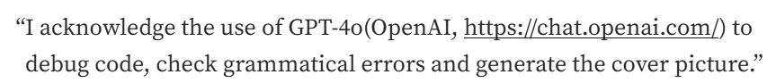
1. When the Sample Mean is Less Than the Population Mean (x_bar < population mean)
If our sample mean (x_bar) is less than the population mean (μ), then many of the points in the sample will be closer to (x_bar) than they would be to μ. As a result, the distances (deviations) from the mean are smaller on average, leading to a smaller variance calculation. This means we’re underestimating the actual variance.
Explanation of the graph given below — The smaller normal distribution is of our sample and the bigger normal distribution is of our population (in the above case where x_bar < population mean), the plot would look like the one shown below.
As we have data points of our sample, because that’s what we can collect, can’t collect all the data points of the population because that’s simply not possible. For all the data points in our sample in this case, from negative infinity, to the mid point of x_bar and population mean, the absolute or squared difference (deviations) between the sample points and population mean would be greater than the absolute or squared difference (deviations) between sample points and sample mean and on the right side of the midpoint till positive infinity, the deviations calculated with respect to sample mean would be greater than the deviations calculated using population mean. The region is indicated in the graph below for the above case, due to the symmetric nature of the normal curve we can surely say that the underestimation zone would be larger than the overestimation zone which is also highlighted in the graph below, which results in an overall underestimation of the deviations.
So to compensate the underestimation, we divide the deviations by a number smaller than sample size ’n’, which is ‘n-1’ which is known as Bessel’s correction.
Plot produced by python code using matplotlib library, Image Source (Author)
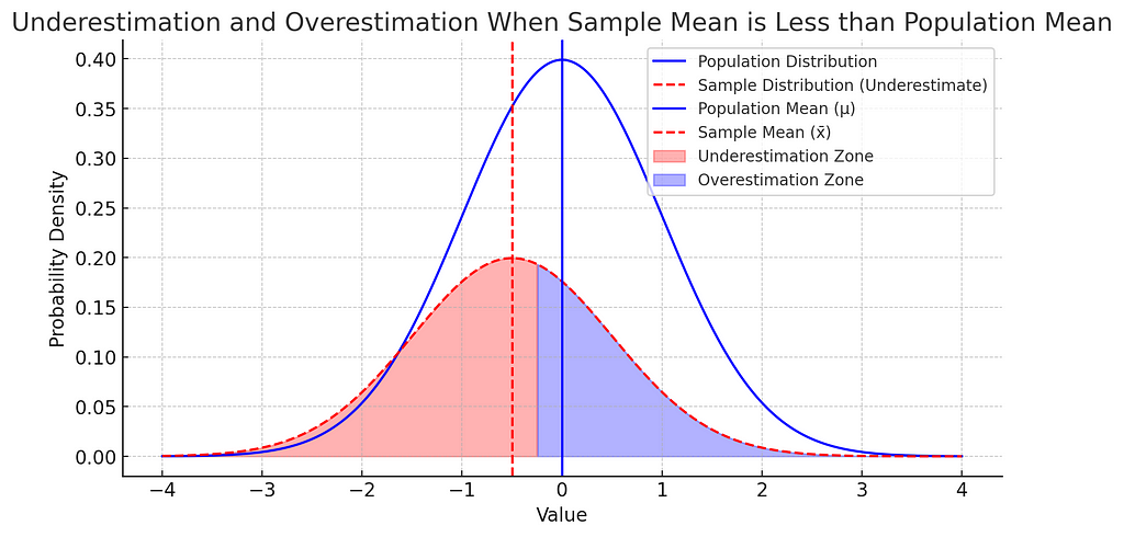
2. When the Sample Mean is Greater Than the Population Mean
If the sample mean is greater than the population mean, we have the reverse situation: data points on the low end of the sample will be closer to x_bar than to μ, still resulting in an underestimation of variance.
Based on the details laid above, it’s clear that in this case also underestimation zone is larger than the overestimation zone, so in this case also we will account for this underestimation by dividing the deviations by ‘n-1’ instead of n.
Plot produced by python code using matplotlib library, Image Source (Author)
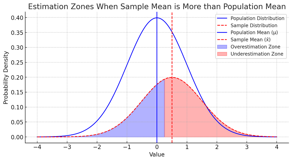
3. When the Sample Mean is Exactly Equal to the Population Mean (0.000001%)
This case is rare, and only if the sample mean is perfectly aligned with the population mean would our estimate be unbiased. However, this alignment almost never happens by chance, so we generally assume that we’re underestimating.
Clearly, deviations calculated for the sample points with respect to sample mean are exactly the same as the deviations calculated with respect to the population mean, because the sample mean and population mean both are equal. This would yield no underestimation or overestimation zone.
Plot produced by python code using matplotlib library, Image Source (Author)
In short, any difference between x_bar and μ (which almost always occurs) leads us to underestimate the variance. This is why we need to make a correction by dividing by n−1, which accounts for this bias.
Why Dividing by n−1 Corrects This Bias: Bessel’s Correction
Dividing by n−1 is called Bessel’s correction and compensates for the natural underestimation bias in sample variance. When we divide by n−1, we’re effectively making a small adjustment that spreads out our variance estimate, making it a better reflection of the true population variance.
One can relate all this to degrees of freedom too , some knowledge of dofs are required to understand from the viewpoint of degrees of freedom-
In a sample, one degree of freedom is “used up” by calculating the sample mean. This leaves us with n−1 independent data points that contribute information about the variance, which is why we divide by n−1 rather than n.
Why Does This Adjustment Matter More with Small Samples?
If our sample size is very small, the difference between dividing by n and n−1 becomes more significant. For instance, if you have a sample size of 10:
Dividing by n would mean dividing by 10, which may greatly underestimate the variance.
Dividing by n−1 or 9, provides a better estimate, compensating for the small sample.
But if your sample size is large (say, 10,000), the difference between dividing by 10,000 or 9,999 is tiny, so the impact of Bessel’s correction is minimal.
Consequences of Not Using Bessel’s Correction
If we don’t use Bessel’s correction, our sample variance will generally underestimate the population variance. This can have cascading effects, especially in statistical modelling and hypothesis testing, where accurate variance estimates are crucial for drawing reliable conclusions.
For instance:
Confidence intervals: Variance estimates influence the width of confidence intervals around a sample mean. Underestimating variance could lead to narrower intervals, giving a false impression of precision.
Hypothesis tests: Many statistical tests, such as the t-test, rely on accurate variance estimates to determine if observed effects are significant. Underestimating variance could make it harder to detect true differences.
Why Not Divide by n−2 or n−3?
The choice to divide by n−1 isn’t arbitrary. While we won’t go into the detailed proof here, it’s grounded in mathematical theory. Dividing by n−1 provides an unbiased estimate of the population variance when calculated from a sample. Other adjustments, such as n−2, would overcorrect and lead to an overestimation of variance.
A Practical Example to Illustrate Bessel’s Correction
Imagine you have a small population with a mean weight of 70 kg. Now let’s say you take a sample of 5 people from this population, and their weights (in kg) are 68, 69, 70, 71, and 72. The sample mean is exactly 70 kg — identical to the population mean by coincidence.
Now suppose we calculate the variance:
Without Bessel’s correction: we’d divide the sum of squared deviations by n=5.
With Bessel’s correction: we divide by n−1=4.
Using Bessel’s correction in this way slightly increases our estimate of the variance, making it closer to what the population variance would be if we calculated it from the whole population instead of just a sample.
Conclusion
Dividing by n−1 when calculating sample variance may seem like a small change, but it’s essential to achieve an unbiased estimate of the population variance. This adjustment, known as Bessel’s correction, accounts for the underestimation that occurs due to relying on the sample mean instead of the true population mean.
In summary:
Using n−1 compensates for the fact that we’re basing variance on a sample mean, which tends to underestimate true variability.
The correction is especially important with small sample sizes, where dividing by n would significantly distort the variance estimate.
This practice is fundamental in statistics, affecting everything from confidence intervals to hypothesis tests, and is a cornerstone of reliable data analysis.
By understanding and applying Bessel’s correction, we ensure that our statistical analyses reflect the true nature of the data we study, leading to more accurate and trustworthy conclusions.
Fastweb, one of Italy’s leading telecommunications operators, recognized the immense potential of AI technologies early on and began investing in this area in 2019. In this post, we explore how Fastweb used cutting-edge AI and ML services to embark on their LLM journey, overcoming challenges and unlocking new opportunities along the way.
We use cookies on our website to give you the most relevant experience by remembering your preferences and repeat visits. By clicking “Accept”, you consent to the use of ALL the cookies.
This website uses cookies to improve your experience while you navigate through the website. Out of these, the cookies that are categorized as necessary are stored on your browser as they are essential for the working of basic functionalities of the website. We also use third-party cookies that help us analyze and understand how you use this website. These cookies will be stored in your browser only with your consent. You also have the option to opt-out of these cookies. But opting out of some of these cookies may affect your browsing experience.
Necessary cookies are absolutely essential for the website to function properly. These cookies ensure basic functionalities and security features of the website, anonymously.
Cookie
Duration
Description
cookielawinfo-checkbox-analytics
11 months
This cookie is set by GDPR Cookie Consent plugin. The cookie is used to store the user consent for the cookies in the category "Analytics".
cookielawinfo-checkbox-functional
11 months
The cookie is set by GDPR cookie consent to record the user consent for the cookies in the category "Functional".
cookielawinfo-checkbox-necessary
11 months
This cookie is set by GDPR Cookie Consent plugin. The cookies is used to store the user consent for the cookies in the category "Necessary".
cookielawinfo-checkbox-others
11 months
This cookie is set by GDPR Cookie Consent plugin. The cookie is used to store the user consent for the cookies in the category "Other.
cookielawinfo-checkbox-performance
11 months
This cookie is set by GDPR Cookie Consent plugin. The cookie is used to store the user consent for the cookies in the category "Performance".
viewed_cookie_policy
11 months
The cookie is set by the GDPR Cookie Consent plugin and is used to store whether or not user has consented to the use of cookies. It does not store any personal data.
Functional cookies help to perform certain functionalities like sharing the content of the website on social media platforms, collect feedbacks, and other third-party features.
Performance cookies are used to understand and analyze the key performance indexes of the website which helps in delivering a better user experience for the visitors.
Analytical cookies are used to understand how visitors interact with the website. These cookies help provide information on metrics the number of visitors, bounce rate, traffic source, etc.
Advertisement cookies are used to provide visitors with relevant ads and marketing campaigns. These cookies track visitors across websites and collect information to provide customized ads.