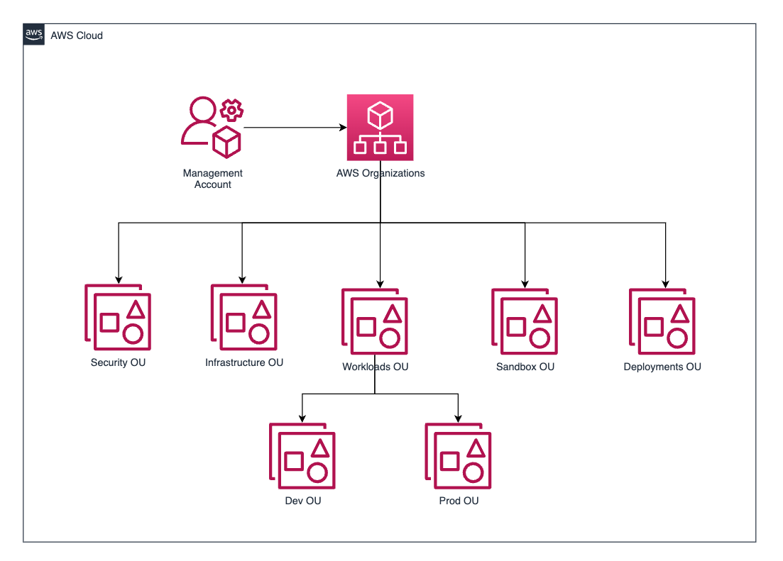
Your multi-account strategy is the core of your foundational environment on AWS. Design decisions around your multi-account environment are critical for operating securely at scale. Grouping your workloads strategically into multiple AWS accounts enables you to apply different controls across workloads, track cost and usage, reduce the impact of account limits, and mitigate the complexity […]
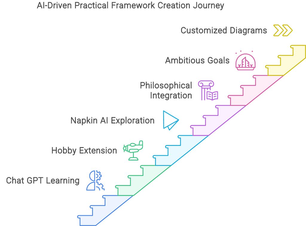
Discover how AI tools can transform intricate concepts into clear, practical frameworks and diagrams
Image by author, made in Napkin AI
Introduction
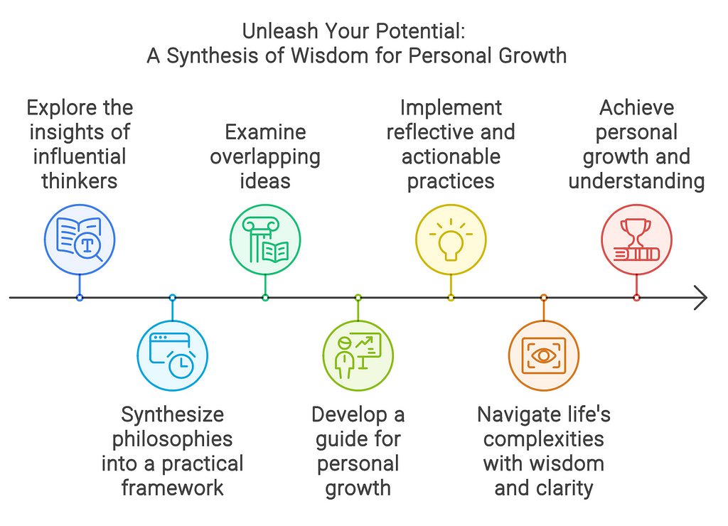
AI tools like Chat GPT are transforming how we approach complex ideas. One of the things I enjoy doing with Chat GPT is integrating perspectives and ideas from different thinkers, as well as differentiating between them to better understand their nuances. This is easily one of my favorite applications of AI.
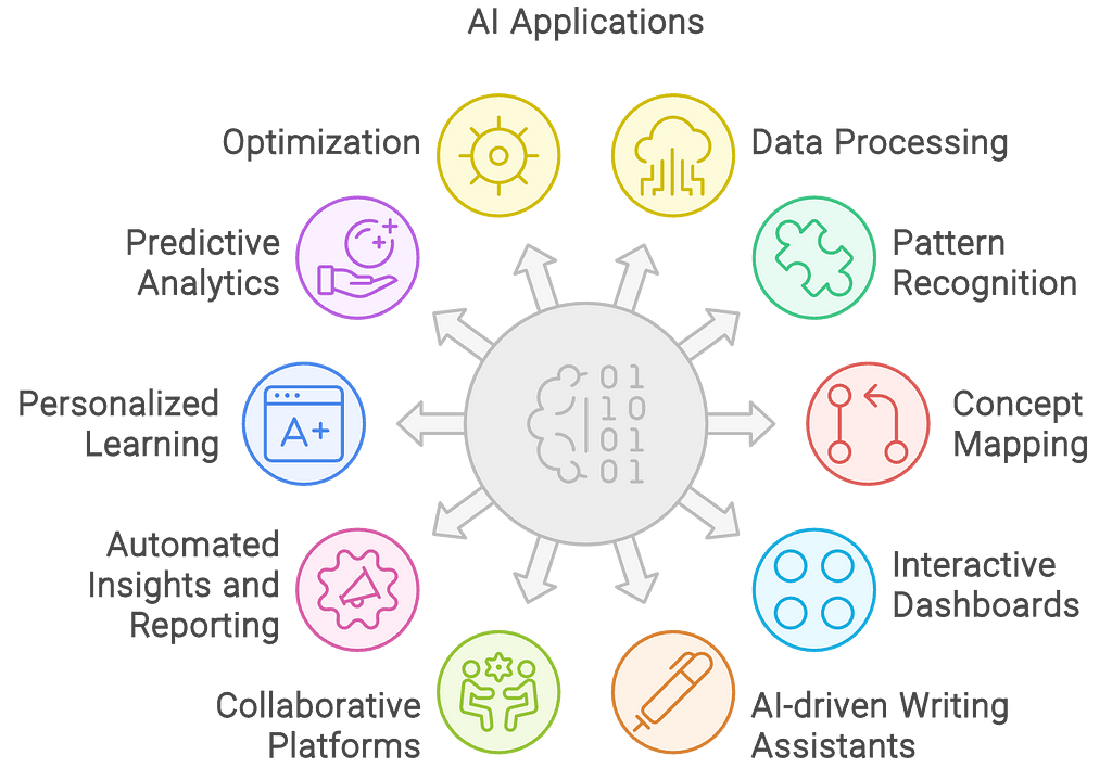
Image by author, made in Napkin AI
Motivation
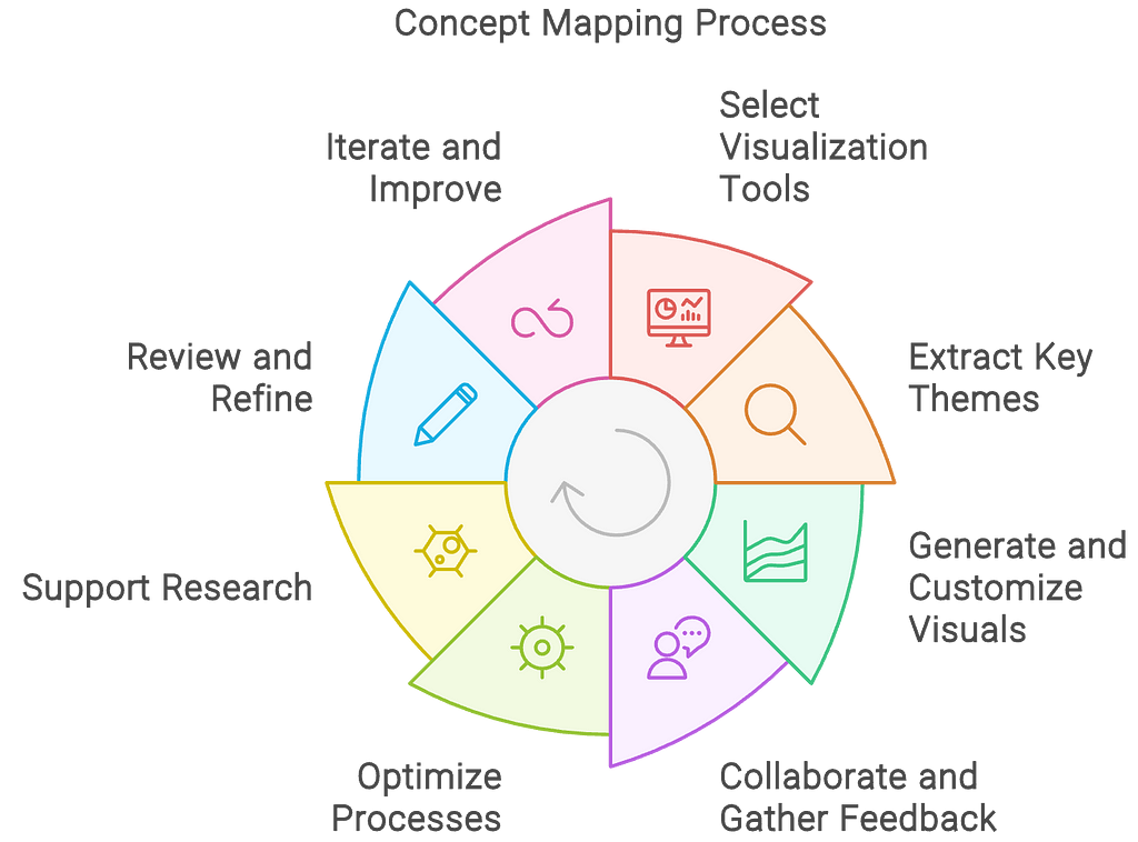
Napkin AI caught my eye because it generates interesting diagrams automatically from text input, making it highly flexible and easy to use. I’ve been looking for good concept mapping and knowledge mapping software, and this seemed like a reasonable place to start.
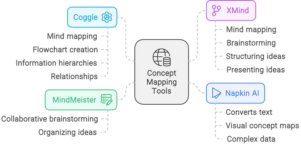
Image by author, made in Napkin AI
Goal
This article is the first in a series where I will explore different methods of examining, integrating, and visualizing complex ideas and perspectives. Although I’ve now moved on to creating my own tool, experimenting with Napkin AI was an important first step. In this series, I will document the journey that will involve exploring some of the tools out there, making new ones easy to use, and sharing my experiences.
Image by author, made in Napkin AI
The Process
1. Setting up the Prompt
After some basic setup, Napkin AI asked me for a prompt. I started with something I happened to be exploring at the time:
“The most unique insights from Alan Watts”
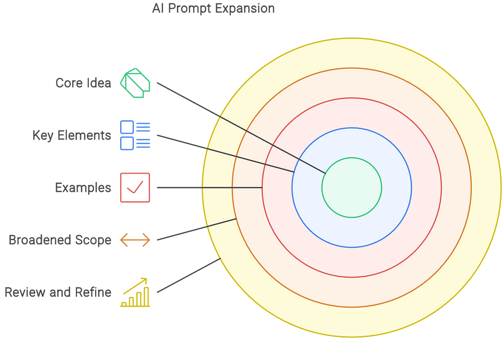
It generated some basic information, maybe about as powerful as Chat GPT-4. I previewed a few diagrams and then decided to challenge it further:
“The most unique insights from Alan Watts, Robert M. Pirsig, Spinoza, and Marcus Aurelius, emphasizing their overlaps with each other and their detailed underpinnings in very specific ideas from philosophy, science, and psychology, organized into practical frameworks and the logical progression towards such frameworks.”
Image by author, made in Napkin AI
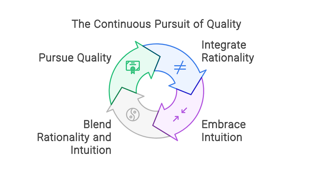
The results were geared more towards the process of creating a framework, which in a broad sense is great, but I wanted it to go further. It was easy enough to start a new Napkin and change a few words of the prompt to focus more on building what I wanted:
… organized into a single practical step by step iterative framework.
2. Creating and Customizing Visuals
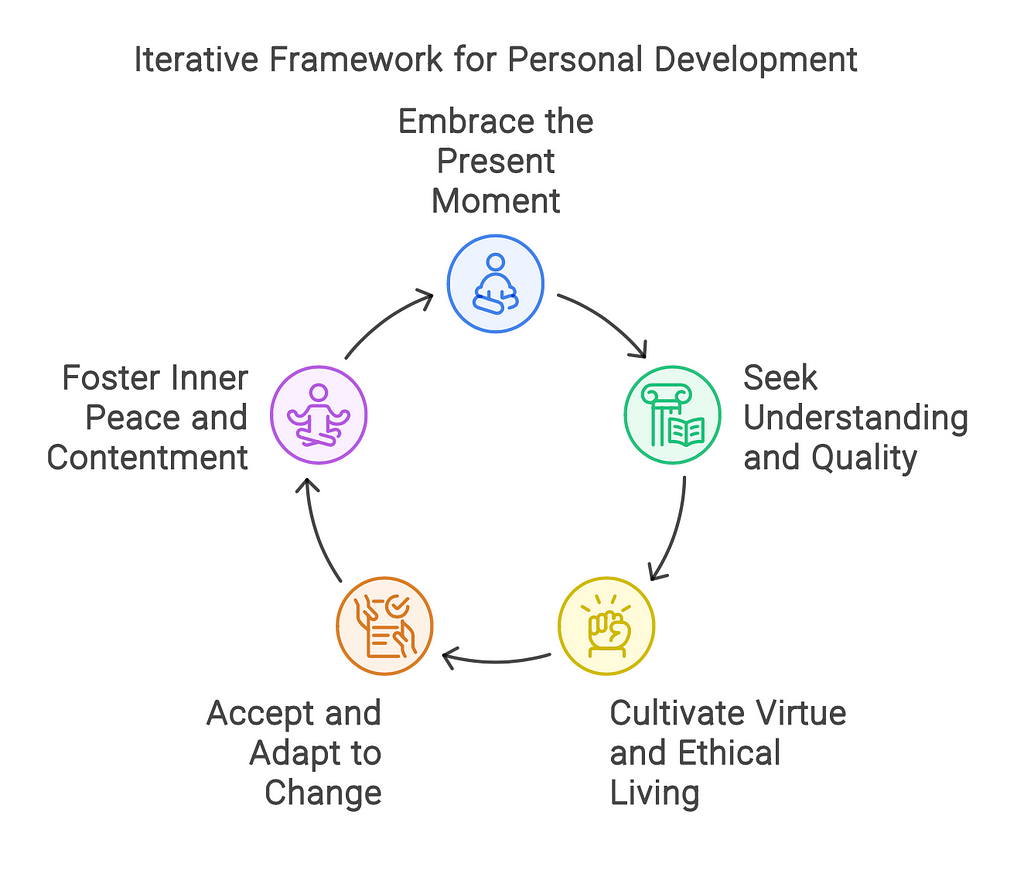
There are a number of templates to choose from, and a few styles. The content of each choice varied slightly, sometimes going into different levels of detail, reflecting the format of the diagram.
I selected the diagram template I felt suited each section best. I tended to prefer a few of the templates that were best suited for this project, but I opted towards a balance between consistency and variety. Here are a few:
Images by author, made in Napkin AI
3. Publishing the Output
Upon completing each document, I exported them as PDFs. Find them here.
Reflections and Applications
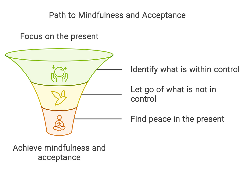
I am definitely glad I went ahead with this tool. What I created is not the type of concept map I was looking for, but it did help me visualize complex topics. It even helped me integrate them into practical frameworks with its Draft with AI option, although you can also start a blank document and provide your own text. If you want to edit the document or add your own images, that’s just as easy.
Image by author, made in Napkin AI
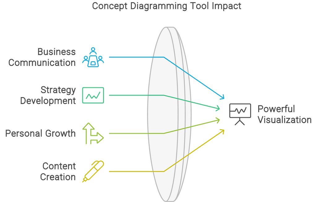
I imagine this could be used in a wide variety of presentational contexts, including business, education, personal growth, and content creation. It empowers individual creators to turn complex ideas into practical frameworks, supporting innovation and growth. Most importantly, it creates powerful diagrams that can be highly useful for business communications and strategy development.
Next Steps
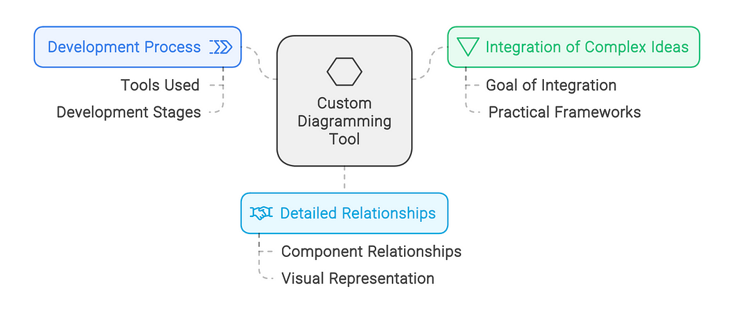
This was a great beginning, but I have more to share. Aside from using other tools for diagramming, I am developing a custom tool tailored to better integrate and visualize complex ideas, including the detailed relationships between their components. This series will cover those journeys. Stay tuned!
Large Language Models (LLMs) have undoubtedly taken the tech industry by storm. Their meteoric rise was fueled by a large corpora of data from Wikipedia, web pages, books, troves of research papers and, of course, user content from our beloved social media platforms. The data and compute hungry models have been feverishly incorporating multi-modal data from audio and video libraries, and have been using 10s of thousands of Nvidia GPUs for months to train the state-of-the-art (SOTA) models. All this makes us wonder whether this exponential growth can last.
The challenges facing these LLMs are numerous but let’s investigate a few here.
Cost and Scalability: Larger models can cost tens of millions of dollars to to train and serve, becoming a barrier to adoption by the swath of day-to-day applications. (See Cost of training GPT-4)
Training Data Saturation: Publicly available datasets will exhaust soon enough and may need to rely on slowly generated user content. Only companies and agencies that have a steady source of new content will be able to generate improvements.
Hallucinations: Models generating false and unsubstantiated information is going to be a deterrent with users expecting validation from authoritative sources before using for sensitive applications.
Exploring unknowns: LLMs are now being used for applications beyond their original intent. For example LLMs have shown great ability in game play, scientific discovery and climate modeling. We will need new approaches to solve these complex situations.
Before we start getting too worried about the future, let’s examine how AI researchers are tirelessly working on ways to ensure continued progress. The Mixture-of-Experts (MoE) and Mixture-of-Agents (MoA) innovations show that hope is on the horizon.
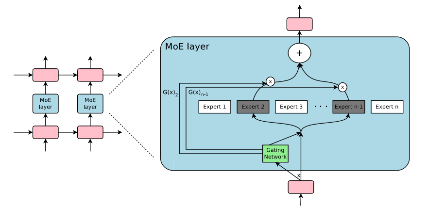
First introduced in 2017, Mixture-of-Experts technique showed that multiple experts and a gating network that can pick a sparse set of experts can produce a vastly improved outcome with lower computational costs. The gating decision allows to turn off large pieces of the network enabling conditional computation, and specialization improves performance for language modeling and machine translational tasks.
Source: MoE Layer from Outrageously Large Neural Networks
The figure above shows that a Mixture-of-Experts layer is incorporated in a recurrent neural network. The gating layer activates only two experts for the task and subsequently combines their output.
While this was demonstrated for select benchmarks, conditional computation has opened up an avenue to see continued improvements without resorting to ever growing model size.
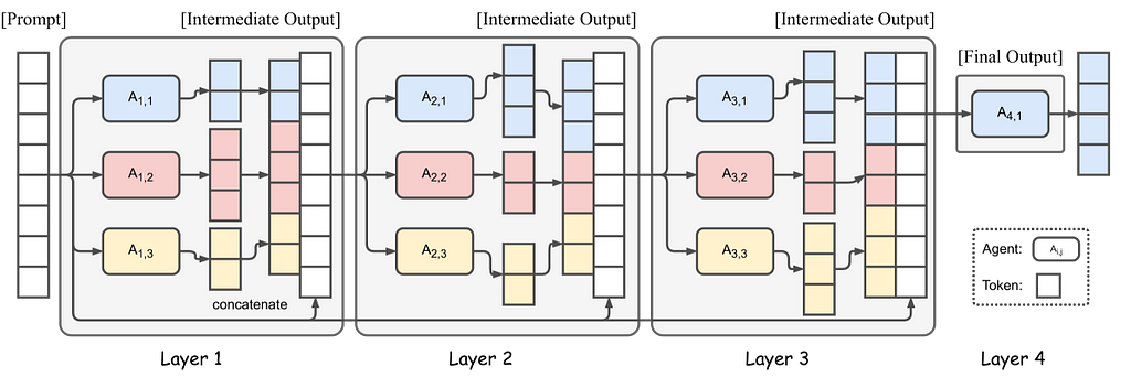
Inspired by MOE, Mixture-of-Agents technique leverages multiple LLM to improve the outcome. The problem is routed through multiple LLMs aka agents that enhance the outcome at each stage and the authors have demonstrated that it produces a better outcome with smaller models versus the larger SOTA models.
Source: Mixture-of-Agents Enhances Large Language Model Capabilities | license
The figure shows 4 Mixture-of-Agents layers with 3 agents in each layer. Selecting appropriate LLMs for each layer is important to ensure proper collaboration and to produce high quality response. (Source)
MOA relies on the fact that LLMs collaborating together produce better outputs as they can combine responses from other models. The role of LLMs is divided into proposers that generate diverse outputs and aggregators that can combine them to produce high-quality responses. The multi-stage approach will likely increase the Time to First Token (TTFT), so mitigating approaches will need to be developed to make them suitable for broad applications.
MOE and MOA have similar foundational elements but behave differently. MOE works on the concept of picking a set of experts to complete a job where the gating network has the task of picking the right set of experts. MOA works on teams building on the work of the previous teams, and improving the outcome at each stage.
Innovations for MOE and MOA have created a path of innovation where a combination of specialized components or models, collaborating and exchanging information, can continue to provide better outcomes even when linear scaling of model parameters and training datasets is no longer trivial.
While it is only with hindsight we will know whether the LLM innovations can last, I have been following the research in the field for insights. Seeing what is coming out of universities and research institutions, I am extremely bullish on what is next to come. I do feel we are just warming up for the onslaught of new capabilities and applications that will transform our lives. We don’t know what they are but we can be fairly certain that coming days will not fail to surprise us.
“We tend to overestimate the effect of a technology in the short run and underestimate the effect in the long run.”. -Amara’s Law
References
[1] Wang, J., Wang, J., Athiwaratkun, B., Zhang, C., & Zou, J. (2024). Mixture-of-Agents Enhances Large Language Model Capabilities. arXiv [Preprint]. https://arxiv.org/abs/2406.04692
[2] Shazeer, N., Mirhoseini, A., Maziarz, K., Davis, A., Le, Q., Hinton, G., & Dean, J. (2017). Outrageously large neural networks: The sparsely-gated mixture-of-experts layer. arXiv preprint arXiv:1701.06538.
I have heard many times data scientists frustrated due to the lack of cool projects to work on within their company. Convincing business stakeholders and management to start AI projects can be challenging. While it is not usually the data scientist’s responsibility to think and propose the projects that need to be prioritized, I’ve seen how data scientists together with data managers and product managers can influence the roadmaps and help introduce more innovative and impactful projects.
In this blog post I am going to share some of the steps and strategies that I’ve seen successfully influence the team or company culture towards introducing more innovative ML or AI based projects. Be aware this is not something that happens from one day to another, but a journey in which your knowledge and motivation can help others in your company to think outside of the box and see the potential of ML and AI.
These key steps and strategies for pitching innovation and AI in your company are: raising awareness, inspiring through use cases, finding sponsors & ideas, and prioritization.
1. Raise awareness about AI
The first step is to raise awareness on your organization about what AI can and cannot do. Many people have limited understanding of AI, which can lead both to skepticism and unrealistic expectations.
The end goal at this first step would be to help people around you to gain sensibility about AI. This sensibility can include: what is the difference between ML and AI, what type of problems can I solve with traditional ML (classification, regression, time series…), what new opportunities appear now with GenAI (text generation, image generation, few shot classification…). Some strategies to reach this awareness are:
Workshops and trainings: these can be organized in-house, or you can also recommend online courses. The second option is usually faster and less expensive; courses like “AI For Everyone” and “Generative AI For Everyone” from deeplearning.ai are always a good start.
Empower & encourage everyone to use GenAI: this can be done by casually explaining how you leverage GenAI yourself, by sharing images and poems obtained through it, or by challenging why they haven’t used it yet. Try to understand if there are specific concerns that are holding people back (e.g. “I don’t trust it with my own data”), and share tools or techniques that can help mitigate those perceived risks.
Showcase ML / AI projects: actively participate in your company demos, All Hands, or internal knowledge sharing sessions. You can share ML or AI projects you or your team have already implemented. It is important to ensure the right level of technical details to allow people to follow your presentation, and highlight the project’s potential, impact, and learnings. It can also be interesting to share how these projects differentiate from “traditional software development” or the other type of projects from the company.
2. Inspire through relevant use cases
People around you have already some awareness and sensibility about AI and ML, the types of models that exist, their potential, and how those types of projects work, great! The next step is to start introducing use cases that can inspire projects for your company. These use cases can come from competitors or analogous industries, but also from the general use cases that apply to most companies (user segmentation, client / user churn prediction, selling forecasts…).
Demonstrating how competitors or other companies are leveraging AI can be powerful to illustrate its potential and inspire next steps. When showcasing use cases, you can focus on the problem that use case solves, the tangible benefits it achieved, and make the analogy on how something similar could be applicable in your company. Similarly, for more general use cases, such as user segmentation, it can be interesting to showcase the type of application that could come out of it in your specific company (dynamic pricing, personalization, improved communications…).
If there are already some teams doing competitors analysis (usually User Researchers), make sure they are also taking into account ML / AI features. Help them gain the sensibility on how those solutions might work underneath to enrich further their research and detect AI opportunities for your company.
There is now awareness on what AI is and what types of problems and use cases it can help solve in your company. If you’ve done it right, you should have been able to get some people really excited about all this potential!
This excitement can translate into people coming directly to you to share other use cases, ask questions, or even ask wether something is feasible to solve with AI or not. These are your sponsors: champions within the organization who can support and advocate for AI initiatives. Depending on the size of the company and how big the culture change needs to be, this sponsorship might be close enough to influence decision-making at the highest levels. However, getting to inspire business stakeholders can also be good enough, as they can push to solve their own objectives through AI.
You’ve planted the seeds for AI project ideas to come out. You can now start proposing specific AI solutions for specific company problems or objectives. Thanks to all the previous work on awareness, use cases, and sponsors, these proposals should be now much more well received!
What is most interesting from this step though, is waiting for the use cases to also come to you. Your AI sponsors and other people in the company are now able to link problems and objectives to AI solutions. It might surprise you how much use cases can appear from this direction. The awareness you’ve built will naturally lead to more informed and relevant suggestions.
4. Assessing and prioritizing use cases
At this point you might have been able to collect several ideas of initiative and have the buy-in from the management to dedicate some time to work on them. But how do you decide with where to start? It might make sense to start with the initiative with biggest potential, but predicting the ROI of innovation, and particularly of AI projects, can be challenging due to their inherent uncertainty. However, there are some key points to take into account that can help on that end:
Focus on specific strategic pain points or opportunities within the company.
Use industry benchmarks to estimate success rates and potential revenues.
Asses potential benefit, but also feasibility and risks.
Differentiate between exploratory (high uncertainty, long-term) and exploitative (low uncertainty, short-term) projects.
Try to start with exploitative ideas (quick wins), to prove value faster, gain traction and build trust. Once that is managed, maybe you can start introducing explorative ideas (moonshots) that aim longer term & bigger transformation, but also involve higher risks to fail. Balancing a continuous delivery and improvement with moonshots is key to maintain the trust long term while also exploring real innovation.
In a previous post “Starting ML Product Initiatives on the Right Foot”, I deep-dived into how to successfully start with ML initiatives and manage their inherent uncertainty from the beginning.
Pitching AI in your company is a long term journey, not something that will happen overnight. From my experience, it is important to start generating awareness and education, showcasing use cases, and aligning with sponsors in the right positions. Only then, proposing use cases will listened; even other people might come to you with relevant ideas! Once some use cases have been gathered and there is some bandwidth and buy-in to prioritize some dedication, it is time to focus on strategic problems, quantify well the opportunity and potential, and balance between quick wins and long term moonshots.
We are in a moment in time where everybody is talking about AI. In particular, companies are trying to think about their (Gen)AI strategies and how this new technology will change the business and ways of working. This plays in your favor: it should be a good moment to start introducing this steps, as people are particularly keen to learn, play, and leverage AI.
From time to time, we all find ourselves considering whether to try out new tooling or experiment with a package, and there’s some risk involved in that. What if the tool doesn’t accomplish what I need, or takes days to get running, or requires complex knowledge I don’t have? Today I’m sharing a simple review of my own experience getting a model up and running using PyTorch Tabular, with code examples that should help other users considering it to get going quickly with a minimum of fuss.
This project began with a pretty high dimensionality CatBoost model, a supervised learning use case with multi-class classification outcome. The dataset has about 30 highly imbalanced classes, which I’ll describe in more detail in a future post. I wanted to try applying a neural network to the same use case, to see what changes in performance I might have, and I came across PyTorch Tabular as a good option. There are of course other alternatives for applying NNs to tabular data, including using base PyTorch yourself, but having a layer on top designed to accommodate your specific problem case often makes things easier and quicker for development. PyTorch Tabular keeps you from having to think about things like how to convert your dataframe to tensors, and gives you a straightforward access point to model customizations.
Getting Started
The documentation at https://pytorch-tabular.readthedocs.io/en/latest/ is pretty easy to read and get into, although the main page points you to the development version of the docs, so keep that in mind if you have installed from pypi.
I use poetry to manage my working environments and libraries, and poetry and PyTorch are known to not get along great all the time, so that’s also a consideration. It definitely took me a few hours to get everything installed and working smoothly, but that’s not the fault of the PyTorch Tabular developers.
As you may have guessed, this is all optimized for tabular data, so I am bringing my engineered features dataset in pandas format. As you’ll see later on, I can just dump dataframes directly into the training function with no need to reformat, provided my fields are all numeric or boolean.
Setup
When you begin structuring your code, you’ll be creating several objects that the PyTorch Tabular training function requires:
DataConfig: prepares the dataloader, including setting up your parallelism for loading.
TrainerConfig: sets batch sizes and epoch numbers, and also lets you determine what processor you’ll use, if you do/don’t want to be on GPU for example.
OptimizerConfig: Allows you to add whatever optimizer you might like, and also a learning rate scheduler, and parameter assignments for each. I didn’t end up customizing this for my use case, it defaults to Adam .
LinearHeadConfig: lets you create the model head if you want to customize that, I didn’t need to add anything special here.
Then you’ll also create a model config, but the base class will differ depending on what kind of model you intend to make. I used the basic CategoryEmbeddingModelConfig for mine, and this is where you’ll assign all the model architecture items such as layer sizes and order, activation function, learning rate, and metrics.
head_config = LinearHeadConfig( layers="", # No additional layer in head, just a mapping layer to output_dim dropout=0.0, initialization="kaiming", ).__dict__ # model config requires dict
Metrics were a little confusing to assign in this section, so I’ll stop and briefly explain. I wanted several different metrics to be visible during training, and in this framework that requires passing several lists for different arguments.
metrics=["f1_score", "average_precision", "accuracy", "auroc"],
metrics_params=[
    {"task": "multiclass", "num_classes": num_classes},
    {"task": "multiclass", "num_classes": num_classes},
    {},
    {},
],  # f1_score and avg prec need num_classes and task identifier
metrics_prob_input=[
    True,
    True,
    False,
    True,
],  # f1_score, avg prec, auroc need probability scores, while accuracy doesn't
Here you can see that I’m returning four metrics, and they each have different implementation requirements, so each list represents the same four metrics and their attributes. For example, average precision needs parameters that indicate that this is a multiclass problem, and it needs to be fed the number of classes involved. It also calls for a probability result instead of raw model outputs, unlike accuracy.
Once you’ve gotten all of this specified, things are pretty easy- you just pass each object into the TabularModel module.
It’s quite easy to set up training once you have train, test, and validation sets created.
tabular_model.fit(train=train_split_df, validation=val_split_df)
result = tabular_model.evaluate(test_split_df)
Training with verbosity on will show you a nice progress bar and keep you informed as to what batch and epoch you’re on. It may tell you, if you’re not using parallelism in your data loader, that there is a data loading bottleneck that you could improve by adding more workers — it’s up to you whether this is of interest, but because my inference job will have a very sparse environment I opted to not have parallelism in my data loader.
Once the training is complete, you can save the model in two different ways — one is as a PyTorch Tabular output, so usable for loading to fine tune or to use for inference in an environment where PyTorch Tabular is available. The other is as an inference-only version, such as a base PyTorch model, which I found very valuable because I needed to use the model object in a much more bare-bones environment for production.
tabular_model.save_model(
  f"data/models/tabular_version_{model_name}"
 ) # The PyTorch Tabular version

tabular_model.save_model_for_inference(
  f"data/models/{model_name}", kind="pytorch"
 ) # The base PyTorch version
There are some other options available for the save_model_for_inference method that you can read about in the docs. Note also that the PyTorch Tabular model object can’t be transferred from CPU to GPU or vice versa on load- you’re going to have to stay on the same compute you used for training, unless you save your model as a PyTorch model object.
Inference
Reloading the model for inference processes later I found really required having both of these objects saved, however, because the PyTorch Tabular model outputs a file called datamodule.sav which is necessary to consistently format your inference data before passing to the model. You could probably put together a pipeline of your own to feed into the model, but I found that to be a much more tedious prospect than just using the file as directed by the documentation. (Note, also, that this file can be rather large- mine turned out over 100mb, and I opted to store it separately rather than just place it with the rest of the code for deployment.)
In PyTorch Tabular there are built in helpers for inference, but I found that getting my multi-class predictions out with the appropriate labels and in a cleanly useful format required pulling out some of the helper code and rewriting it in my own codebase. For non-multiclass applications, this might not be necessary, but if you do end up going that way, this is the script I adapted from.
This is how the inference process then looks in code, with feature engineering etc omitted. (This runs in Docker on AWS Lambda.)
point_predictions = [] for batch in tqdm(inference_dataloader, desc="Generating Predictions..."): for k, v in batch.items(): print("New Batch") if isinstance(v, list) and (len(v) == 0): continue batch[k] = v.to(pytorch_model.device) y_hat, ret_value = pytorch_model.predict(batch, ret_model_output=True) point_predictions.append(y_hat.detach().cpu())
After this point, the predictions are formatted and softmax applied to get the probabilities of the different classes, and I can optionally reattach the predictions to the original dataset for evaluation purposes later.
Conclusions
Overall, I was really pleased with how PyTorch Tabular works for my use case, although I’m not sure whether I’m going to end up deploying this model to production. My biggest challenges were ensuring that my training process was properly designed so that the inference task (mainly the dataloader) would work efficiently in my production environment, but once I resolved that things were fine. Frankly, not having to think much about formatting tensors was worth the time, too!
So, if you want to try adapting a model from classical frameworks like CatBoost or LightGBM, I’d recommend giving PyTorch Tabular a try—if nothing else, it should be pretty quick to get up and running, so your experimentation turnaround won’t be too tedious. Next time, I’ll write about what exactly I was using PyTorch Tabular for, and describe performance metrics for the same underlying problem comparing CatBoost at PyTorch.
Deep Dive into Multi-Head Attention, the secret element in Transformers and LLMs. Let’s explore its math, and build it from scratch in Python
Image generated by DALL-E
1: Introduction
1.1: Transformers Overview
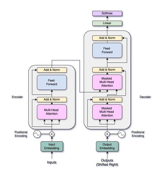
The Transformer architecture, introduced by Vaswani et al. in their paper “Attention is All You Need” has transformed deep learning, particularly in natural language processing (NLP). Transformers use a self-attention mechanism, enabling them to handle input sequences all at once. This parallel processing allows for faster computation and better management of long-range dependencies within the data. This doesn’t sound familiar? Don’t worry as it will be at the end of this article. Let’s first take a brief look at what a Transformer looks like.
A Transformer consists of two main parts: an encoder and a decoder. The encoder processes the input sequence to create a continuous representation, while the decoder generates the output sequence from this representation. Both the encoder and the decoder have multiple layers, each containing two essential components: a multi-head self-attention mechanism and a position-wise feed-forward network. In this article, we’ll focus on the multi-head attention mechanism, but we’ll explore the entire Transformer architecture in future articles.
1.2: Multi-Head Attention Overview
Multi-head attention enables the model to focus on different parts of the input sequence at the same time, capturing various aspects of the data. Think of it like having multiple spotlights shining on different parts of a stage. Each spotlight (or “head”) can illuminate a different performer (or data feature), allowing the audience (or model) to see the whole scene more clearly. By splitting the input into multiple subspaces, each with its attention mechanism, multi-head attention provides the model with several views of the input data. This setup helps the model understand complex relationships within the data more effectively.
This mechanism allows the Transformer to capture different relationships in the data by attending to various parts of the sequence. This improves the learning process by offering multiple perspectives of the input, enhancing the model’s ability to generalize. It also increases the model’s expressiveness by enabling it to learn different aspects of the input data simultaneously.
These capabilities make multi-head attention a crucial component in the success of Transformer models across a range of applications, from language translation to image processing.
2: The Mathematical Foundations
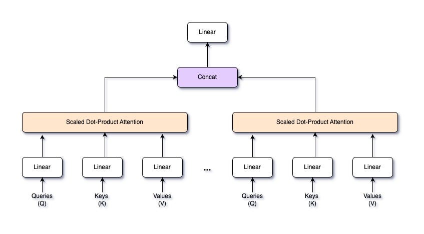
Multi-Head Attention Architecture — Image by Author
2.1: Attention Mechanism
The attention mechanism in neural networks is designed to mimic the human ability to focus on specific parts of information while processing data. Imagine reading a book: your eyes don’t pay equal attention to every word on the page. Instead, they focus more on the important words that help you understand the story. Similarly, in neural networks, attention allows the model to dynamically weigh the importance of different input elements. This means the model can prioritize parts of the input sequence that are more relevant for generating the output, improving its performance in tasks like language translation, text summarization, and more.
Mathematically, the attention mechanism can be described using a set of queries, keys, and values. Let’s denote the input as a set of queries Q, keys K, and values V. These are typically linear transformations of the input data.
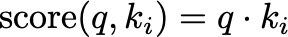
The attention scores are calculated by taking the dot product of the query with all keys, which gives a measure of similarity. For a query q and a set of keys k1, k2, …, kn, the attention scores are given by:
Attention Score — Image by Author
Think of this as comparing how similar each word (key) in a sentence is to the word (query) you’re focusing on. Higher scores indicate greater similarity.
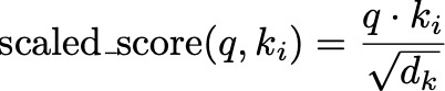
To prevent the dot products from becoming too large, especially when dealing with high-dimensional vectors, we scale the scores by the square root of the dimension of the keys, d_k:
Scaled Score Formula — Image by Author
This is like adjusting the intensity of the spotlight based on how large the stage is. It ensures that the scores remain manageable and helps maintain stable gradients during training. This scaling ensures that the values passed to the softmax function have a standard deviation close to 1, which helps maintain stable gradients during training.
To see why this is necessary, consider the properties of dot products and high-dimensional vectors. When we compute the dot product of two vectors q and k_i of dimension d_k, the expected value of their dot product is proportional to d_k. Without scaling, as d_k increases, the variance of the dot product grows, leading to very large values which can cause the softmax function to produce near-binary outputs (i.e., probabilities close to 0 or 1). This sharpness reduces the model’s ability to learn effectively because it makes the gradients very small.
By dividing the dot product by d_k, we normalize the input to the softmax function, ensuring that the scores remain within a reasonable range. This normalization helps the model to maintain a balance, enabling it to learn more effectively and stably.
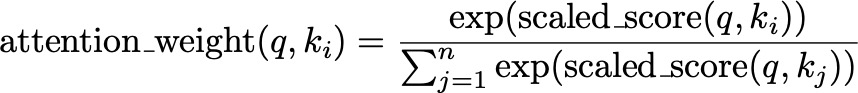
These scaled scores are then passed through a softmax function to obtain the attention weights. The softmax function converts the scores into probabilities, which represent the importance of each key relative to the query:
Attention Weight using Softmax Function — Image by Author
This step is like converting the adjusted spotlight intensities into a clear ranking, highlighting the most relevant parts of the scene more brightly.
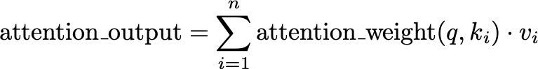
The final attention output is obtained by taking a weighted sum of the values, using the attention weights:
Attention Output Formula — Image by Author
Here, v_i represents the value corresponding to key k_i. This weighted sum combines the most relevant information from the values, much like focusing your attention on the most important parts of the book to understand the story better.
2.2: Multi-Head Attention
Multi-head attention is an advanced form of the attention mechanism that allows a model to focus on different parts of the input sequence simultaneously, capturing various relationships within the data. Instead of having a single attention mechanism, multi-head attention splits the input into multiple “heads,” each with its own set of queries, keys, and values. Each head performs the attention operation independently, and their outputs are then combined. This enhances the model’s ability to understand complex patterns and dependencies in the data.
Imagine you’re trying to understand a complex scene with many elements. If you had multiple pairs of eyes, each looking at different parts of the scene, you’d get a more comprehensive understanding. Similarly, multi-head attention allows the model to focus on different parts of the input data at once, providing a richer and more detailed representation.
Given an input sequence X, we project it into queries Q, keys K, and values V using learned linear transformations. For each head i, we have separate weight matrices W_Q, W_K, and W_V:
Queries, Keys, and Values Linear Transformations — Image by Author
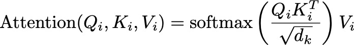
These projections allow each head to focus on different aspects of the input data. For each head i, we compute the attention scores using the scaled dot-product attention mechanism. The attention output for head i is:
Attention Formula — Image by Author
Here, d_k is the dimension of the key vectors, ensuring the scores are appropriately scaled.
After computing the attention outputs for all heads, we concatenate them along the feature dimension. If we have h heads, each producing an output of dimension d_v, the concatenated output will have a dimension of h×d_v:
Multi-Head Concatenation — Image by Author
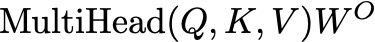
The concatenated output is then projected back to the original input dimension d using a learned weight matrix W_O:
Final Layer of Multi-Head Attention — Image by Author
This final linear transformation combines the outputs from all heads into a single representation.
The core idea behind combining multiple attention heads is to allow the model to capture different types of information from the input sequence simultaneously. By having multiple heads, each head can learn to attend to different parts of the input or different features. This diversity in attention leads to a richer and more nuanced representation of the data.
2.3: Position-wise Feed-Forward Networks
In the Transformer architecture, each layer consists of a multi-head attention mechanism followed by a position-wise feed-forward network. These feed-forward layers are applied independently to each position in the sequence, hence the term “position-wise.” Essentially, they are simple fully connected neural networks applied separately and identically to each position of the input sequence.
Imagine a factory where every product on the conveyor belt goes through the same set of machines. Each machine processes the product in a specific way, adding something new or refining it. Similarly, each position in the sequence is processed independently by the feed-forward layers, transforming and enhancing the representation.
The purpose of these feed-forward layers is to introduce non-linearity and additional learning capacity to the model. After the attention mechanism has aggregated information from different parts of the sequence, the feed-forward network processes this information to further transform and refine the representation.
Mathematically, a position-wise feed-forward network consists of two linear transformations with a ReLU activation function in between. Given an input x at a particular position, the feed-forward network can be represented as:
Feed-Forward Network Formula — Image by Author
Here:
W1 and W2 are learned weight matrices.
b1 and b2 are learned bias vectors.
max(0, xW1+b1) represents the ReLU activation function applied element-wise.
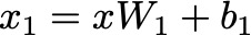
The input x is first linearly transformed using the weight matrix W1 and bias b1:
Linear Transformation of the input — Image by Author
Think of this step as passing the input through the first machine in the factory, which adds initial modifications based on learned weights and biases.
The linear transformation is followed by a ReLU activation function, which introduces non-linearity:
ReLU Formula — Image by Author
ReLU (Rectified Linear Unit) sets all negative values to zero, allowing the model to capture non-linear relationships in the data. This step is like ensuring only positive contributions from the first machine are passed on.
The activated output is then passed through a second linear transformation using weight matrix W2 and bias b2:
Second FFN — Image by Author
This final step further refines the output, much like the second machine in the factory making additional modifications to produce a finished product.
The position-wise feed-forward network in the Transformer architecture further processes the information captured by the multi-head attention mechanism. While the attention mechanism allows the model to focus on different parts of the sequence and aggregate context-specific information, the feed-forward network refines and transforms this information at each position. This enhances the model’s ability to capture complex patterns and dependencies.
3: Building Multi-Head Attention from Scratch
In this section, we will break down and explain the implementation of a multi-head attention mechanism from scratch using Python and numpy. The goal is to understand how the input is modified during the process. Before proceed with your reading, take a look at the code we will cover in this section. You should be able to get a general understanding, but don’t worry if now, as we will go over each line in this section.
To begin, we define the MultiHeadAttention class, which is responsible for managing the parameters needed for the multi-head attention mechanism. Let’s go through this step-by-step to understand how we set it up.
In the initialization method, we first set the number of attention heads and the total number of hidden units in the model. These values are provided as arguments when the class is instantiated.
num_hiddens: This represents the total number of hidden units in the model. It’s a crucial parameter because it determines the size of the linear transformations applied to the input data.
num_heads: This indicates the number of attention heads. Each head will independently learn to focus on different parts of the input, enabling the model to capture various aspects of the data.
dropout: This is the dropout rate, which is not used in this particular implementation but is included for completeness.
bias: This is a boolean flag indicating whether to include biased terms in the linear transformations.
We then calculate the dimensions of the queries and values for each head. Since the total number of hidden units (num_hiddens) is split across all heads (num_heads), each head will have a query and value dimension of num_hiddens // num_heads.
Next, we initialize the weight matrices for the queries, keys, values, and output transformations. These weight matrices are randomly initialized:
W_q is used to transform the input data into queries. It has dimensions num_hiddens x num_hiddens, meaning it maps the input features to the query space.
W_k is used to transform the input data into keys. It also has dimensions num_hiddens x num_hiddens, mapping the input features to the key space.
W_v is used to transform the input data into values, with the same dimensions as the previous matrices.
W_o is used to transform the concatenated output of all heads back to the original input dimensions.
Finally, we initialize the bias vectors for the queries, keys, values, and output transformations. If the bias parameter is set to True, these biases are randomly initialized. Otherwise, they are set to zero:
b_q: Bias for the query transformation.
b_k: Bias for the key transformation.
b_v: Bias for the value transformation.
b_o: Bias for the output transformation.
The biases have dimensions equal to the number of hidden units, num_hiddens.
By setting up these weights and biases, we ensure that each attention head can independently learn to focus on different parts of the input data.
Next, we define methods to prepare and transform the data for multi-head attention. First, let’s look at the transpose_qkv method:
def transpose_qkv(self, X):
    X = X.reshape(X.shape[0], X.shape[1], self.num_heads, -1)
    X = X.transpose(0, 2, 1, 3)
    return X.reshape(-1, X.shape[2], X.shape[3])
This method is responsible for reshaping and transposing the input data to prepare it for multi-head attention. In particular:
X = X.reshape(X.shape[0], X.shape[1], self.num_heads, -1)
This line reshapes the input tensor X to have four dimensions: (batch_size, sequence_length, num_heads, depth_per_head).
X.shape[0] is the batch size.
X.shape[1] is the sequence length (number of positions in the input sequence).
self.num_heads is the number of attention heads.
-1 automatically infers the size of the last dimension (depth per head) so that the total number of elements remains the same.
X = X.transpose(0, 2, 1, 3)
This line transposes the tensor so that the dimensions are reordered to (batch_size, num_heads, sequence_length, depth_per_head).
This rearrangement ensures that each attention head processes its part of the input sequence independently.
return X.reshape(-1, X.shape[2], X.shape[3])
This final reshape flattens the batch and head dimensions into a single dimension, resulting in a tensor of shape (batch_size * num_heads, sequence_length, depth_per_head).
By doing this, transpose_qkv ensures that the input data is split correctly among the multiple heads, with each head having the appropriate dimensions to process its segment of the data.
Next, we have the transpose_output method:
def transpose_output(self, X):
    X = X.reshape(-1, self.num_heads, X.shape[1], X.shape[2])
    X = X.transpose(0, 2, 1, 3)
    return X.reshape(X.shape[0], X.shape[1], -1)
This method reverses the transformation done by transpose_qkv to combine the outputs from all heads back into the original shape.
After transposing our matrices, we can process with the scaled dot-product attention mechanism, which allows the model to focus on different parts of the input sequence with varying degrees of importance.
The inputs to this method are the query (Q), key (K), and value (V) matrices. These matrices are derived from the input data through linear transformations.
d_k = Q.shape[-1]
Here, we extract the dimension of the key vectors, d_k, from the last dimension of the query matrix Q. This value is used for scaling the attention scores.
We calculate the attention scores by performing a matrix multiplication of Q and the transpose of K. The scores are then scaled by the square root of d_k. This scaling helps prevent the scores from growing too large, which can lead to issues during the softmax calculation.
Next, we define the forward pass method to process the input data through the multi-head attention mechanism. This method is crucial as it orchestrates the entire multi-head attention process, from transforming the input data to combining the outputs from multiple heads.
First, the input queries, keys, and values are projected into their respective subspaces using the learned weight matrices (W_q, W_k, W_v) and biases (b_q, b_k, b_v). This is done by performing matrix multiplication with the weight matrices and adding the biases. The results are then transformed for multi-head attention using the transpose_qkv method, which reshapes and transposes the data to ensure each head processes the input independently.
Queries, keys, and values are the transformed inputs, now prepared for multi-head attention.
if valid_lens is not None:
    valid_lens = np.repeat(valid_lens, self.num_heads, axis=0)
If valid_lens (valid lengths) are provided, they are repeated for each head. This ensures that the appropriate mask is created for each attention head, allowing the model to focus only on valid positions within the sequences.
The method then calls scaled_dot_product_attention with the transformed queries, keys, values, and repeated valid lengths. This function calculates the attention scores, applies the softmax function to obtain attention weights, and computes the weighted sum of the values to produce the attention output for each head.
After obtaining the attention outputs from all heads, the method concatenates these outputs along the feature dimension using transpose_output. This method reverses the initial transformation, combining the outputs from all heads back into a single representation. The concatenated output is then transformed back to the original input dimension using a final linear transformation with weight matrix W_o and bias b_o.
Lastly, we test the class with some sample data. Here’s how we do it:
We initialize the MultiHeadAttention class with 100 hidden units and 5 attention heads. This sets up the necessary parameters and weight matrices for the multi-head attention mechanism.
# Define sample data
batch_size, num_queries, num_kvpairs = 2, 4, 6
valid_lens = np.array([3, 2])
X = np.random.rand(batch_size, num_queries, num_hiddens)  # Use random data to simulate input queries
Y = np.random.rand(batch_size, num_kvpairs, num_hiddens)  # Use random data to simulate key-value pairs
We create random data to simulate input queries (X) and key-value pairs (Y). The batch size is 2, the number of queries is 4, and the number of key-value pairs is 6. We also define valid lengths (valid_lens) to indicate the valid positions within the sequences.
# Apply multi-head attention
output = attention.forward(X, Y, Y, valid_lens)
We pass the sample data through the multi-head attention mechanism using the forward method. This processes the input queries, keys, and values, applying the multi-head attention calculations.
print("Output shape:", output.shape)
# Output should be: (2, 4, 100)

print("Output data:", output)
We print the shape and content of the output. The expected output shape ensures that the output dimensions match the original input dimensions. Then, we print the output data after computing Multi-Head Attention. Now that you have an understanding of how the Multi-Head Attention mechanism works, try tweaking it. For instance, change the number of heads, try adding multiple FFN before and after Multi-Head Attention. Also, you could try to implement it in a machine translation task, and see it in action. Let me know if you would like me to do that in a next article.
Conclusion
Transformers have transformed deep learning, especially in NLP, by using self-attention mechanisms that allow for parallel processing of input sequences. This approach not only speeds up computation but also handles long-range dependencies more effectively than traditional recurrent neural networks).
In this article, we’ve gained a comprehensive understanding of multi-head attention in Transformers, from it’s math theory to a practical code implementation. Maybe for now the concepts we will still be abstracts, as you can’t really do anything with the outputs from Multi-Head Attention, but soon we will see how they play a key role in the transformer architecture, which is the base of the well-known LLMs around (Claude, ChatGPT, …). Stay tuned for future articles, where we’ll explore the remaining components of the Transformer architecture, offering deeper insights into this powerful model.
References
Vaswani, A., Shazeer, N., Parmar, N., Uszkoreit, J., Jones, L., Gomez, A. N., Kaiser, Ł., & Polosukhin, I. (2017). Attention is All You Need. In Advances in Neural Information Processing Systems (NeurIPS).
An end-2-end empirical sharing of multi-step quantile forecasting with Tensorflow, NeuralForecast, and Zero-shot LLMs.
Image by Author
Content
Short Introduction
Data
Build a Toy Version of Quantile Recurrent Forecaster
Quantile Forecasting with the State-of-Art Models
Zero-shot Quantile Forecast with LLMs
Conclusion
Short Introduction
Quantile forecasting is a statistical technique used to predict different quantiles (e.g., the median or the 90th percentile) of a response variable’s distribution, providing a more comprehensive view of potential future outcomes. Unlike traditional mean forecasting, which only estimates the average, quantile forecasting allows us to understand the range and likelihood of various possible results.
Quantile forecasting is essential for decision-making in contexts with asymmetric loss functions or varying risk preferences. In supply chain management, for example, predicting the 90th percentile of demand ensures sufficient stock levels to avoid shortages, while predicting the 10th percentile helps minimize overstock and associated costs. This methodology is particularly advantageous in sectors such as finance, meteorology, and energy, where understanding distribution extremes is as critical as the mean.
Both quantile forecasting and conformal prediction address uncertainty, yet their methodologies differ significantly. Quantile forecasting directly models specific quantiles of the response variable, providing detailed insights into its distribution. Conversely, conformal prediction is a model-agnostic technique that constructs prediction intervals around forecasts, guaranteeing that the true value falls within the interval with a specified probability. Quantile forecasting yields precise quantile estimates, whereas conformal prediction offers broader interval assurances.
The implementation of quantile forecasting can markedly enhance decision-making by providing a sophisticated understanding of future uncertainties. This approach allows organizations to tailor strategies to different risk levels, optimize resource allocation, and improve operational efficiency. By capturing a comprehensive range of potential outcomes, quantile forecasting enables organizations to make informed, data-driven decisions, thereby mitigating risks and enhancing overall performance.
Data
To demonstrate the work, I chose to use the data from the M4 competition as an example. The data is under CC0: Public Domain license which can be accessed here. The data can also be loaded through datasetsforecast package:
# Install the package
pip install datasetsforecast
# Load Data
df, *_ = M4.load('./data', group='Weekly')
# Randomly select three items
df = df[df['unique_id'].isin(['W96', 'W100', 'W99'])]
# Define the start date (for example, "1970-01-04")
start_date = pd.to_datetime("1970-01-04")
# Convert 'ds' to actual week dates
df['ds'] = start_date + pd.to_timedelta(df['ds'] - 1, unit='W')
# Display the DataFrame
df.head()
Image by Author
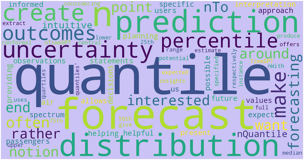
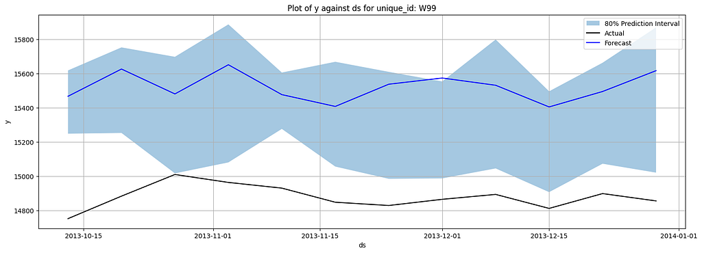
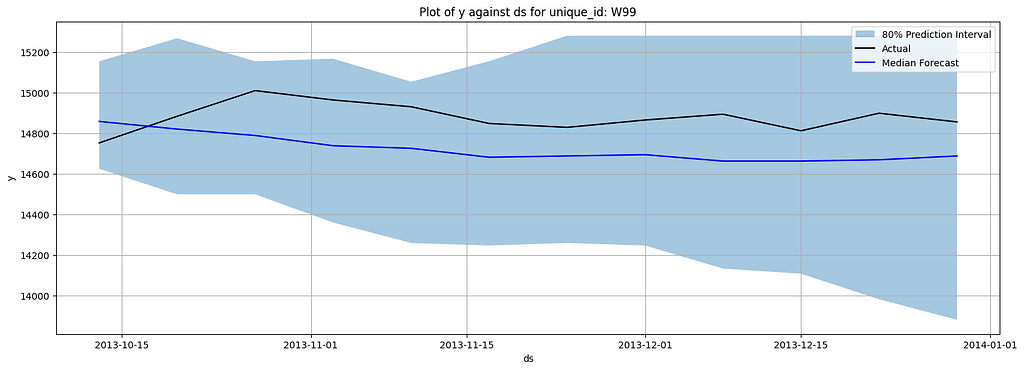
The original data contains over 300 unique time series. To demonstrate, I randomly selected three time series: W96, W99, and W100, as they all have the same history length. The original timestamp is masked as integer numbers (i.e., 1–2296), I manually converted it back to normal date format with the first date to be January 4th, 1970. The following figure is a preview of W99:
Image by Author
Build a Toy Version of Quantile Recurrent Forecaster
First, let’s build a quantile forecaster from scratch to understand how the target data flows through the pipeline and how the forecasts are generated. I picked the idea from the paper A Multi-Horizon Quantile Recurrent Forecaster by Wen et al. The authors proposed a Multi-Horizon Quantile Recurrent Neural Network (MQ-RNN) framework that combines Sequence-to-Sequence Neural Networks, Quantile Regression, and Direct Multi-Horizon Forecasting for accurate and robust multi-step time series forecasting. By leveraging the expressiveness of neural networks, the nonparametric nature of quantile regression, and a novel training scheme called forking-sequences, the model can effectively handle shifting seasonality, known future events, and cold-start situations in large-scale forecasting applications.
We cannot reproduce everything in this short blog, but we can try to replicate part of it using the TensorFlow package as a demo. If you are interested in the implementation of the paper, there is an ongoing project that you can leverage: MQRNN.
Let’s first load the necessary package and define some global parameters. We will use the LSTM model as the core, and we need to do some preprocessing on the data to obtain the rolling windows before fitting. The input_shape is set to (104, 1) meaning we are using two years of data for each training window. In this walkthrough, we will only look into an 80% confidence interval with the median as the point forecast, which means the quantiles = [0.1, 0.5, 0.9]. We will use the last 12 weeks as a test dataset, so the output_steps or horizon is equal to 12 and the cut_off_date will be ‘2013–10–13’.
# Install the package pip install tensorflow
# Load the package from sklearn.preprocessing import StandardScaler from datetime import datetime from tensorflow.keras.models import Model from tensorflow.keras.layers import Input, LSTM, Dense, concatenate, Layer
Next, let’s convert the data to rolling windows which is the desired input shape for RNN-based models:
# Preprocess The Data
def preprocess_data(df, window_size = 104, forecast_horizon = 12):
    # Ensure the dataframe is sorted by item and date

    df = df.sort_values(by=['unique_id', 'ds'])
    # List to hold processed data for each item
    X, y, unique_id, ds = [], [], [], []
    # Normalizer
    scaler = StandardScaler()
    # Iterate through each item
    for key, group in df.groupby('unique_id'):
        demand = group['y'].values.reshape(-1, 1)
        scaled_demand = scaler.fit_transform(demand)
        dates = group['ds'].values
        # Create sequences (sliding window approach)
        for i in range(len(scaled_demand) - window_size - forecast_horizon + 1):
            X.append(scaled_demand[i:i+window_size])
            y.append(scaled_demand[i+window_size:i+window_size+forecast_horizon].flatten())
            unique_id.append(key)
            ds.append(dates[i+window_size:i+window_size+forecast_horizon])
    X = np.array(X)
    y = np.array(y)
    return X, y, unique_id, ds, scaler
Then we split the data into train, val, and test:
# Split Data def split_data(X, y, unique_id, ds, cut_off_date): cut_off_date = pd.to_datetime(cut_off_date) val_start_date = cut_off_date - pd.Timedelta(weeks=12) train_idx = [i for i, date in enumerate(ds) if date[0] < val_start_date] val_idx = [i for i, date in enumerate(ds) if val_start_date <= date[0] < cut_off_date] test_idx = [i for i, date in enumerate(ds) if date[0] >= cut_off_date]
train_unique_id = [unique_id[i] for i in train_idx] train_ds = [ds[i] for i in train_idx] val_unique_id = [unique_id[i] for i in val_idx] val_ds = [ds[i] for i in val_idx] test_unique_id = [unique_id[i] for i in test_idx] test_ds = [ds[i] for i in test_idx]
The authors of the MQRNN utilized both horizon-specific local context, essential for temporal awareness and seasonality mapping, and horizon-agnostic global context to capture non-time-sensitive information, enhancing the stability of learning and the smoothness of generated forecasts. To build a model that sort of reproduces what the MQRNN is doing, we need to write a quantile loss function and add layers that capture local context and global context. I added an attention layer to it to show you how the attention mechanism can be included in such a process:
# Quantile Loss Function def quantile_loss(q, y_true, y_pred): e = y_true - y_pred return tf.reduce_mean(tf.maximum(q*e, (q-1)*e))
def combined_quantile_loss(quantiles, y_true, y_pred, output_steps): losses = [quantile_loss(q, y_true, y_pred[:, i*output_steps:(i+1)*output_steps]) for i, q in enumerate(quantiles)] return tf.reduce_mean(losses)
# Model architecture def create_model(input_shape, quantiles, output_steps): inputs = Input(shape=input_shape) lstm1 = LSTM(256, return_sequences=True)(inputs) lstm_out, state_h, state_c = LSTM(256, return_sequences=True, return_state=True)(lstm1) context_vector, attention_weights = Attention(256)(state_h, lstm_out) global_context = Dense(100, activation = 'relu')(context_vector) forecasts = [] for q in quantiles: local_context = concatenate([global_context, context_vector]) forecast = Dense(output_steps, activation = 'linear')(local_context) forecasts.append(forecast) outputs = concatenate(forecasts, axis=1) model = Model(inputs, outputs) model.compile(optimizer='adam', loss=lambda y, f: combined_quantile_loss(quantiles, y, f, output_steps)) return model
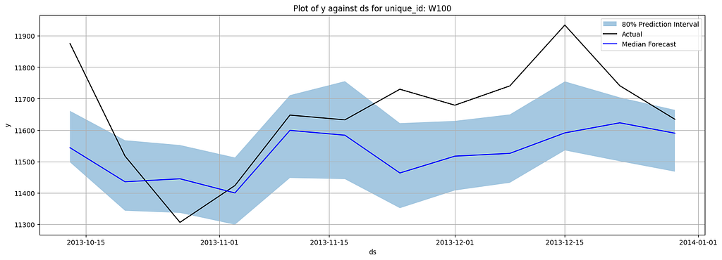
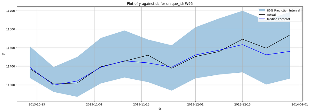
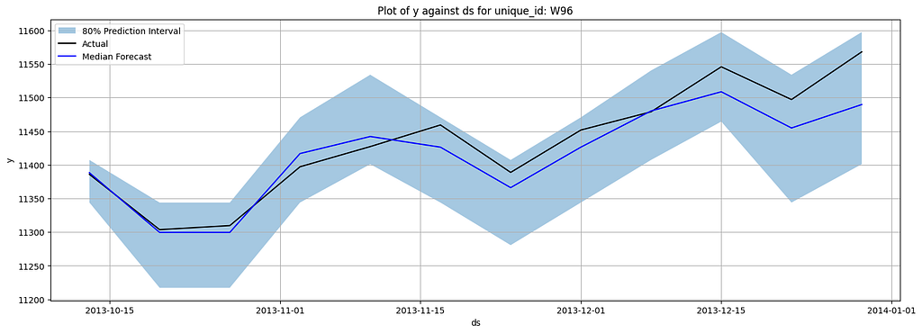
Here are the plotted forecasting results:
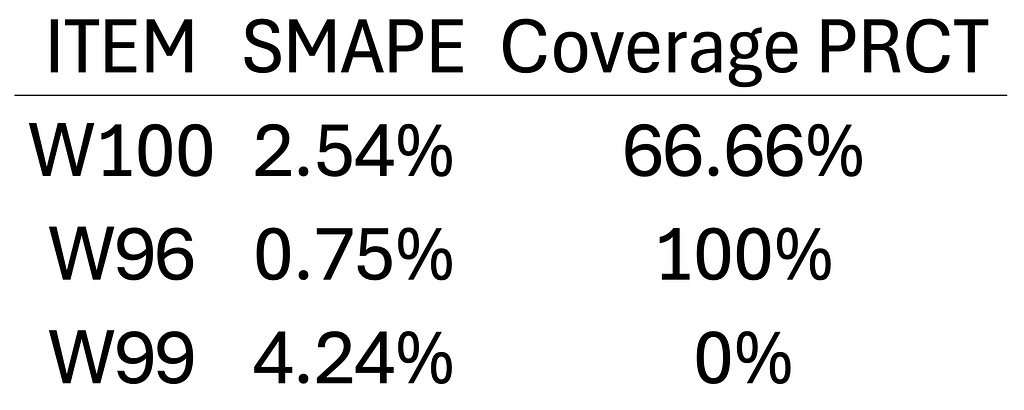
We also evaluated the SMAPE for each item, as well as the percentage coverage of the interval (how much actual was covered by the interval). The results are as follows:
This toy version can serve as a good baseline to start with quantile forecasting. The distributed training is not configured for this setup nor the model architecture is optimized for large-scale forecasting, thus it might suffer from speed issues. In the next section, we will look into a package that allows you to do quantile forecasts with the most advanced deep-learning models.
Quantile Forecasting with the SOTA Models
The neuralforecast package is an outstanding Python library that allows you to use most of the SOTA deep neural network models for time series forecasting, such as PatchTST, NBEATs, NHITS, TimeMixer, etc. with easy implementation. In this section, I will use PatchTST as an example to show you how to perform quantile forecasting.
First, load the necessary modules and define the parameters for PatchTST. Tuning the model will require some empirical experience and will be project-dependent. If you are interested in getting the potential-optimal parameters for your data, you may look into the auto modules from the neuralforecast. They will allow you to use Ray to perform hyperparameter tuning. And it is quite efficient! The neuralforecast package carries a great set of models that are based on different sampling approaches. The ones with the base_window approach will allow you to use MQLoss or HuberMQLoss, where you can specify the quantile levels you are looking for. In this work, I picked HuberMQLoss as it is more robust to outliers.
# Install the package
pip install neuralforecast

# Load the package
from neuralforecast.core import NeuralForecast
from neuralforecast.models import PatchTST
from neuralforecast.losses.pytorch import HuberMQLoss, MQLoss

# Define Parameters for PatchTST
PARAMS = {'input_size': 104,
          'h': output_steps,
          'max_steps': 6000,
          'encoder_layers': 4,
          'start_padding_enabled': False,
          'learning_rate': 1e-4,
          'patch_len': 52,  # Length of each patch
          'hidden_size': 256,  # Size of the hidden layers
          'n_heads': 4,  # Number of attention heads
          'res_attention': True,
          'dropout': 0.1,  # Dropout rate
          'activation': 'gelu',  # Activation function
          'dropout': 0.1,
          'attn_dropout': 0.1,
          'fc_dropout': 0.1,
          'random_seed': 20240710,
          'loss': HuberMQLoss(quantiles=[0.1, 0.5, 0.9]),
          'scaler_type': 'standard',
          'early_stop_patience_steps': 10}

# Get Training Data
train_df = df[df.ds<cut_off_date]

# Fit and predict with PatchTST
models = [PatchTST(**PARAMS)]
nf = NeuralForecast(models=models, freq='W')
nf.fit(df=train_df, val_size=12)
Y_hat_df = nf.predict().reset_index()
Here are plotted forecasts:
Here are the metrics:
Through the demo, you can see how easy to implement the model and how the performance of the model has been lifted. However, if you wonder if there are any easier approaches to do this task, the answer is YES. In the next section, we will look into a T5-based model that allows you to conduct zero-shot quantile forecasting.
Zero-shot Quantile Forecast with LLMs
We have been witnessing a trend where the advancement in NLP will also further push the boundaries for time series forecasting as predicting the next word is a synthetic process for predicting the next period’s value. Given the fast development of large language models (LLMs) for generative tasks, researchers have also started to look into pre-training a large model on millions of time series, allowing users to do zero-shot forecasts.
However, before we draw an equal sign between the LLMs and Zero-shot Time Series tasks, we have to answer one question: what is the difference between training a language model and training a time series model? It would be “tokens from a finite dictionary versus values from an unbounded.” Amazon recently released a project called Chronos which well handled the challenge and made the large time series model happen. As the authors stated: “Chronos tokenizes time series into discrete bins through simple scaling and quantization of real values. In this way, we can train off-the-shelf language models on this ‘language of time series,’ with no changes to the model architecture”. The original paper can be found here.
Currently, Chronos is available in multiple versions. It can be loaded and used through the autogluon API with only a few lines of code.
# Get Training Data and Transform train_df = df[df.ds<cut_off_date] train_df_chronos = TimeSeriesDataFrame(train_df.rename(columns={'ds': 'timestamp', 'unique_id': 'item_id', 'y': 'target'}))
As you can see, Chronos showed a very decent performance compared to PatchTST. However, it does not mean it has surpassed PatchTST, since it is very likely that Chronos has been trained on M4 data. In their original paper, the authors also evaluated their model on the datasets that the model has not been trained on, and Chronos still yielded very comparable results to the SOTA models.
There are many more large time series models being developed right now. One of them is called TimeGPT which was developed by NIXTLA. The invention of this kind of model not only made the forecasting task easier, more reliable, and consistent, but it is also a good starting point to make reasonable guesses for time series with limited historical data.
Conclusion
From building a toy version of a quantile recurrent forecaster to leveraging state-of-the-art models and zero-shot large language models, this blog has demonstrated the power and versatility of quantile forecasting. By incorporating models like TensorFlow’s LSTM, NeuralForecast’s PatchTST, and Amazon’s Chronos, we can achieve accurate, robust, and computationally efficient multi-step time series forecasts. Quantile forecasting not only enhances decision-making by providing a nuanced understanding of future uncertainties but also allows organizations to optimize strategies and resource allocation. The advancements in neural networks and zero-shot learning models further push the boundaries, making quantile forecasting a pivotal tool in modern data-driven industries.
Note: All the images, numbers and tables are generated by the author. The complete code can be found here: Quantile Forecasting.
Using a GloVe embedding-based algorithm to achieve 100% accuracy on the popular party game “Codenames”
Introduction
Codenames is a popular party game for 2 teams of 2 players each, where each team consists of a spymaster and an operative. Each team is allocated a number of word cards on a game board. During each turn, the spymaster provides a word clue, and the number of word cards it corresponds to. The operative would then have to guess which words on the game board belong to his/her team. The objective is for the spymaster to provide good clues, such that the operative can use fewer number of turns to guess all the words, before the opponent team. In addition, there will be an “assassin” card, which upon being chosen by the operative, causes the team to lose immediately.
In this project, we are going to use a simple word vector algorithm using pre-trained word vectors in machine learning to maximize our accuracy in solving the game in as few tries as possible.
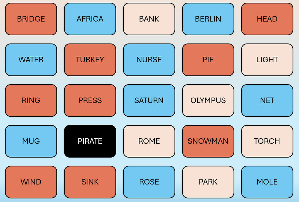
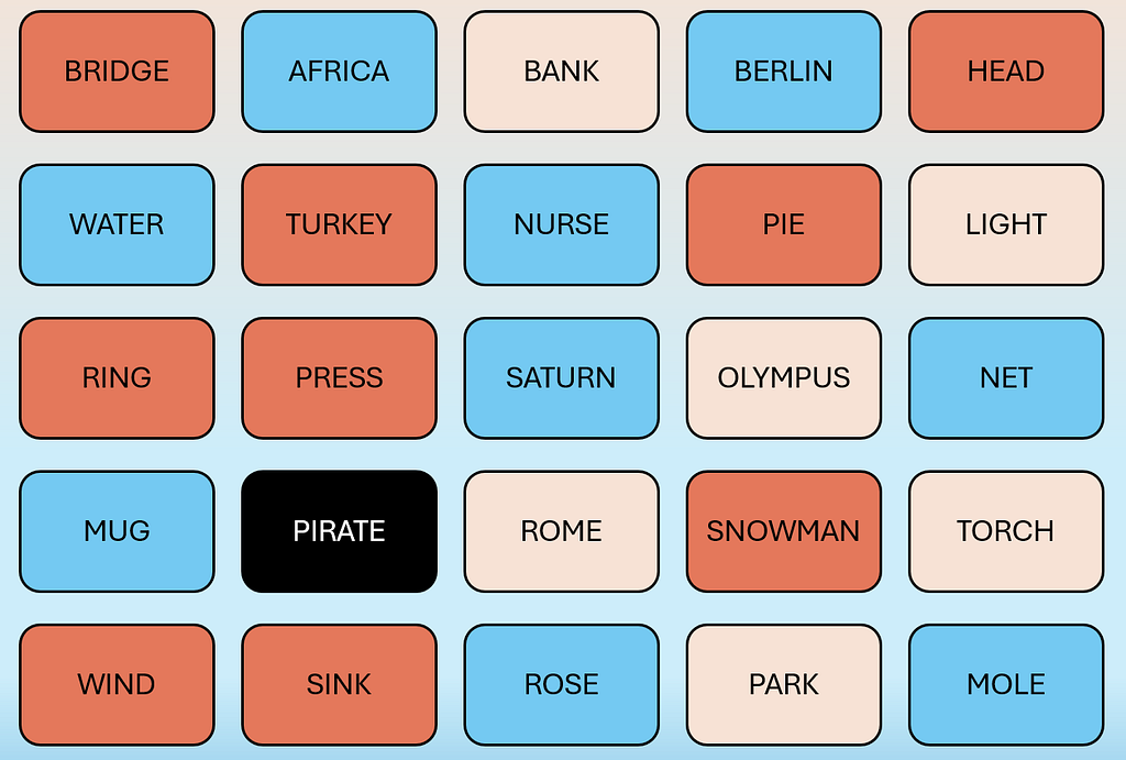
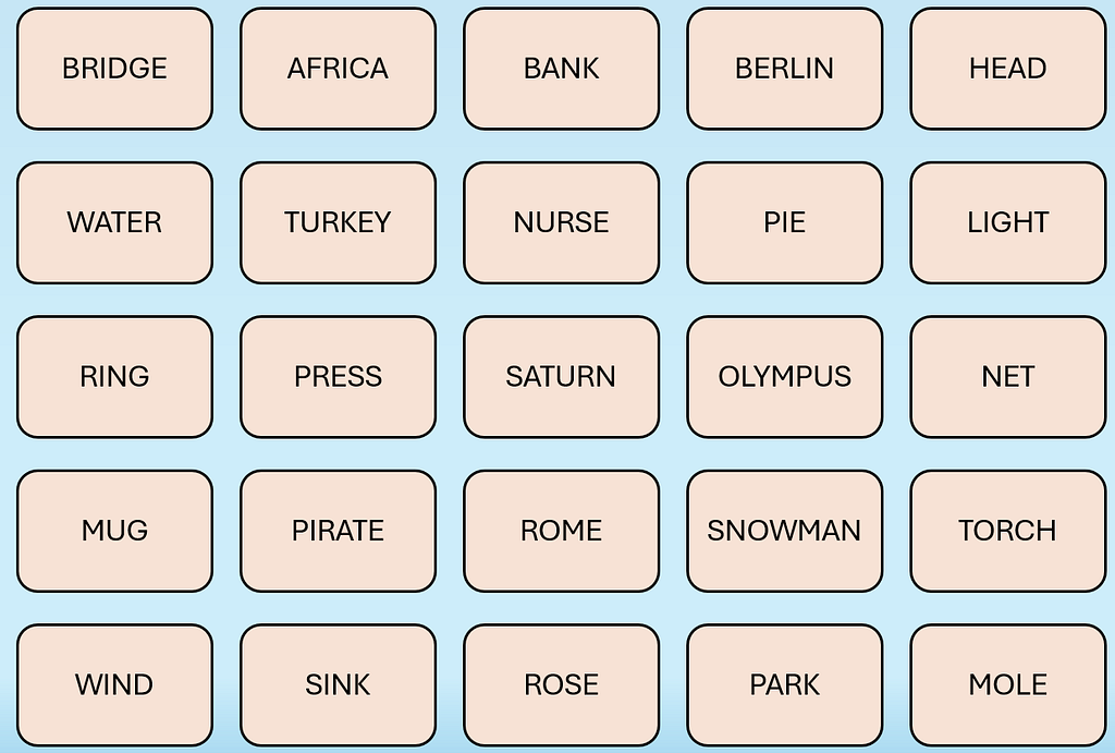
Below are examples of what the game board looks like:
Spymaster View (Image by author)Operative View (Image by author)
In the card arrangement for the Spymaster, the color of each card represents Red Team, Blue Team, Neutral (Beige) and Assassin Card (Black).
Automating the spymaster and operative
We will be creating an algorithm that can take on both the roles of spymaster and operative and play the game by itself. In a board of 25 cards, there will be 9 “good” cards and 16 “bad” cards (including 1 “assassin” card).
Representing meaning with GloVe embeddings
In order for the spymaster to give good clues to the operative, our model needs to be able to understand the meaning of each word. One popular way to represent word meaning is via word embeddings. For this task, we will be using pre-trained GloVe embeddings, where each word is represented by a 100-dimensional vector.
We then score the similarity between two words using cosine similarity, which is the dot product of two vectors divided by their magnitudes:
Image by author
Operative: Decoding Algorithm
During each turn, the operative receives a clue c, and an integer n representing the number of corresponding words to guess. In other words, the operator has to decode a {c, n} pair and choose n words one at a time without replacement, until a wrong word is reached and the turn ends.
Our decoder is a straightforward greedy algorithm: simply sort all the remaining words on the board based on cosine similarity with the clue word c, and pick the top n words based on similarity score.
Spymaster: Encoding Algorithm
On each turn, based on the remaining “good” and “bad” words, the spymaster has to pick n words and decide on a clue c to give to the operative. One assumption we make here is that the spymaster and operative agree on the decoding strategy mentioned above, and hence the operator will pick the optimal {c, n} that will maximize the number of correct words chosen.
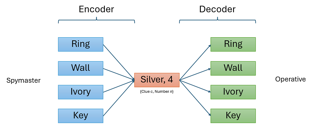
At this point, we can make an observation that the clue c is an information bottleneck, because it has to summarize n words into a single word c for the operative to decode. The word vector of the encoded clue lies in the same vector space as each of the original word vectors.
Mechanics of encoder-decoder system (Image by author)
Generating clue candidates
Word embeddings have the property of enabling us to represent composite meanings via the addition and subtraction of different word vectors. Given set of “good” words G and set of “bad” words B, we can use this property to obtain an “average” meaning of a “good” word, with reference to the “bad” words, by computing a normalized mean of the vectors, with “good” word vectors being added, and “bad” word vectors being subtracted. This average vector enables us to generate clue candidates:
As the number of “bad” words usually exceeds the number of “good” words, we perform negative sampling, by randomly sampling an equal number of “bad” words compared to the “good” words in our computation of our average word vector. This also contributes to more randomness in the clues generated, which improves the diversity of clue candidates.
After we find the average word vector, we use the most_similar() function in Gensim to obtain the top closest words from the entire GloVe vocabulary with respect to the average word vector, based on cosine similarity.
Score function
Now, we have a method to generate candidates for clue c, given n words. However, we still have to decide which candidate c to pick, which n words to choose, and how to determine n.
Thereafter, we generate all possible combinations of k, k-1, …, 1 words from the k “good” words remaining on the board, as well as their respective clue word candidates c, working backwards from k. To pick the best {c, n},we score all the candidates from each possible combination of the remaining “good” words, through the decoding algorithm. Then we obtain the maximum number of words guessed correct given clue c, count(c), since we know what strategy the operative will use.
Image by author
Results
In each game, 25 words are sampled from a list of 400 common Codenames words. Overall, after 100 experiments, our method chooses the correct word 100% of the time, completing the game within an average of 1.98 turns, or 4.55 guesses per turn (for 9 correct words), taking at most 2 turns.
Average number of guesses at each turn as game progresses (Image by author)
In other words, this algorithm takes two turns almost every game, except for a few exceptions where it guesses all the words in a single turn.
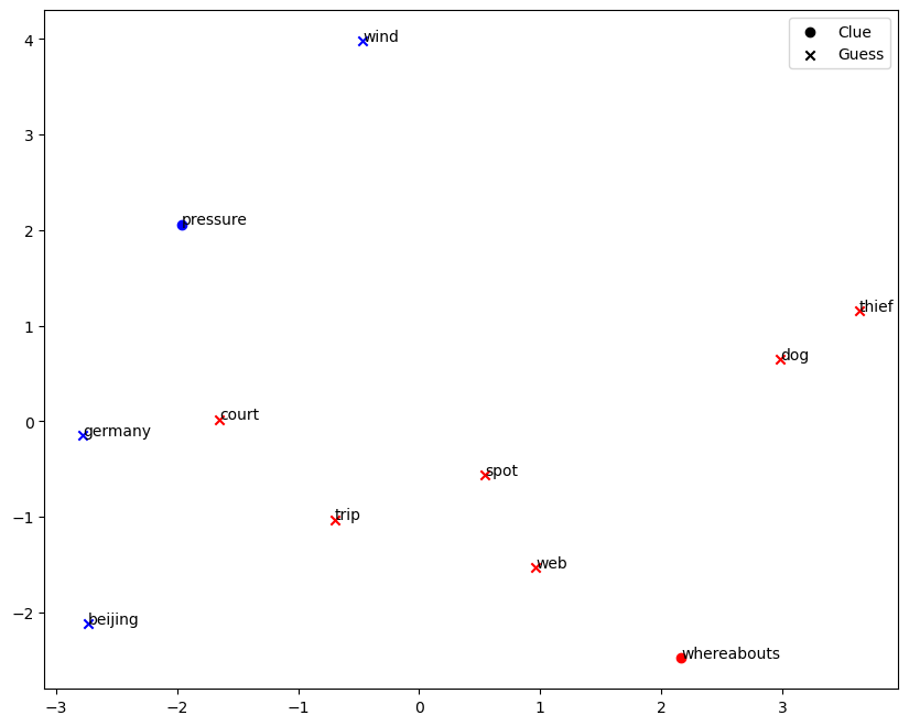
Let’s view a sample distribution of word embeddings of the clues and guesses we made.
Scatter plot of word embeddings for 1 game after PCA reduction (Image by author)
Although the clues generated do provide some level of semantic summary of the words that the operative eventually guessed correctly, these relationships between clues and guesses may not be obvious from a human perspective. One way to make to clues more interpretable is to cap the maximum number of guesses per turn, which generates clues with better semantic approximation of the guesses.
Even so, our algorithm promotes a good clustering outcome for each of the words, to enable our decoder to get more words correct by providing good clues that lie close to the target words.
Conclusion
In conclusion, this greedy GloVe-based algorithm performs well as both the spymaster and operative in the Codenames game, by offering an effective way to encode and decode words via a clue and number.
In our model, the encoder and decoder share a common strategy, which works in similar ways as a shared encryption key. A possible limitation of this is that the encoder and decoder will not work as well separately, as a human player may not be able to interpret the generated clues as effectively.
Understanding the mechanics behind word embeddings and vector manipulation is a great way to get started in Natural Language Processing. It is interesting to see how simple methods can also perform well in such semantic clustering and classification tasks. To enhance the gameplay even further, one can consider using adding elements of reinforcement learning or training an autoencoder to achieve better results.
Koyyalagunta, D., Sun, A., Draelos, R. L., & Rudin, C. (2021). Playing codenames with language graphs and word embeddings. Journal of Artificial Intelligence Research, 71, 319–346. https://doi.org/10.1613/jair.1.12665
Pennington, J., Socher, R., & Manning, C. (2014). Glove: Global vectors for word representation. Proceedings of the 2014 Conference on Empirical Methods in Natural Language Processing (EMNLP). https://doi.org/10.3115/v1/d14-1162
Jaramillo, C., Charity, M., Canaan , R., & Togelius, J. (2020). Word Autobots: Using Transformers for Word Association in the Game Codenames. Proceedings of the AAAI Conference on Artificial Intelligence and Interactive Digital Entertainment, 16(1), 231–237. https://doi.org/10.1609/aiide.v16i1.7435
We use cookies on our website to give you the most relevant experience by remembering your preferences and repeat visits. By clicking “Accept”, you consent to the use of ALL the cookies.
This website uses cookies to improve your experience while you navigate through the website. Out of these, the cookies that are categorized as necessary are stored on your browser as they are essential for the working of basic functionalities of the website. We also use third-party cookies that help us analyze and understand how you use this website. These cookies will be stored in your browser only with your consent. You also have the option to opt-out of these cookies. But opting out of some of these cookies may affect your browsing experience.
Necessary cookies are absolutely essential for the website to function properly. These cookies ensure basic functionalities and security features of the website, anonymously.
Cookie
Duration
Description
cookielawinfo-checkbox-analytics
11 months
This cookie is set by GDPR Cookie Consent plugin. The cookie is used to store the user consent for the cookies in the category "Analytics".
cookielawinfo-checkbox-functional
11 months
The cookie is set by GDPR cookie consent to record the user consent for the cookies in the category "Functional".
cookielawinfo-checkbox-necessary
11 months
This cookie is set by GDPR Cookie Consent plugin. The cookies is used to store the user consent for the cookies in the category "Necessary".
cookielawinfo-checkbox-others
11 months
This cookie is set by GDPR Cookie Consent plugin. The cookie is used to store the user consent for the cookies in the category "Other.
cookielawinfo-checkbox-performance
11 months
This cookie is set by GDPR Cookie Consent plugin. The cookie is used to store the user consent for the cookies in the category "Performance".
viewed_cookie_policy
11 months
The cookie is set by the GDPR Cookie Consent plugin and is used to store whether or not user has consented to the use of cookies. It does not store any personal data.
Functional cookies help to perform certain functionalities like sharing the content of the website on social media platforms, collect feedbacks, and other third-party features.
Performance cookies are used to understand and analyze the key performance indexes of the website which helps in delivering a better user experience for the visitors.
Analytical cookies are used to understand how visitors interact with the website. These cookies help provide information on metrics the number of visitors, bounce rate, traffic source, etc.
Advertisement cookies are used to provide visitors with relevant ads and marketing campaigns. These cookies track visitors across websites and collect information to provide customized ads.


