An open-source, model-agnostic agentic framework that supports dependency injection
Ideally, you can evaluate agentic applications even as you are developing them, instead of evaluation being an afterthought. For this to work, though, you need to be able to mock both internal and external dependencies of the agent you are developing. I am extremely excited by PydanticAI because it supports dependency injection from the ground up. It is the first framework that has allowed me to build agentic applications in an evaluation-driven manner.
Image of Krakow Cloth Hall, generated using Google Imagen by the author. This building was built in phases over the centuries, with improvements based on where the current building was falling short. Evaluation-driven development, in other words.
In this article, I’ll talk about the core challenges and demonstrate developing a simple agent in an evaluation-driven way using PydanticAI.
Challenges when developing GenAI applications
Like many GenAI developers, I’ve been waiting for an agentic framework that supports the full development lifecycle. Each time a new framework comes along, I try it out hoping that this will be the One — see, for example, my articles about DSPy, Langchain, LangGraph, and Autogen.
I find that there are core challenges that a software developer faces when developing an LLM-based application. These challenges are typically not blockers if you are building a simple PoC with GenAI, but they will come to bite you if you are building LLM-powered applications in production.
What challenges?
(1) Non-determinism: Unlike most software APIs, calls to an LLM with the exact same input could return different outputs each time. How do you even begin to test such an application?
(2) LLM limitations: Foundational models like GPT-4, Claude, and Gemini are limited by their training data (e.g., no access to enterprise confidential information), capability (e.g., you can not invoke enterprise APIs and databases), and can not plan/reason.
(3) LLM flexibility: Even if you decide to stick to LLMs from a single provider such as Anthropic, you may find that you need a different LLM for each step — perhaps one step of your workflow needs a low-latency small language model (Haiku), another requires great code-generation capability (Sonnet), and a third step requires excellent contextual awareness (Opus).
(4) Rate of Change: GenAI technologies are moving fast. Recently, many of the improvements have come about in foundational model capabilities. No longer are the foundational models just generating text based on user prompts. They are now multimodal, can generate structured outputs, and can have memory. Yet, if you try to build in an LLM-agnostic way, you often lose the low-level API access that will turn on these features.
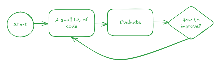
To help address the first problem, of non-determinism, your software testing needs to incorporate an evaluation framework. You will never have software that works 100%; instead, you will need to be able to design around software that is x% correct, build guardrails and human oversight to catch the exceptions, and monitor the system in real-time to catch regressions. Key to this capability is evaluation-driven development (my term), an extension of test-driven development in software.
Evaluation-driven development. sketch by author.
The current workaround for all the LLM limitations in Challenge #2 is to use agentic architectures like RAG, provide the LLM access to tools, and employ patterns like Reflection, ReACT and Chain of Thought. So, your framework will need to have the ability to orchestrate agents. However, evaluating agents that can call external tools is hard. You need to be able to inject proxies for these external dependencies so that you can test them individually, and evaluate as you build.
To handle challenge #3, an agent needs to be able to invoke the capabilities of different types of foundational models. Your agent framework needs to be LLM-agnostic at the granularity of a single step of an agentic workflow. To address the rate of change consideration (challenge #4), you want to retain the ability to make low-level access to the foundational model APIs and to strip out sections of your codebase that are no longer necessary.
Is there a framework that meets all these criteria? For the longest time, the answer was no. The closest I could get was to use Langchain, pytest’s dependency injection, and deepeval with something like this (full example is here):
from unittest.mock import patch, Mock from deepeval.metrics import GEval
llm_as_judge = GEval( name="Correctness", criteria="Determine whether the actual output is factually correct based on the expected output.", evaluation_params=[LLMTestCaseParams.INPUT, LLMTestCaseParams.ACTUAL_OUTPUT], model='gpt-3.5-turbo' )
@patch('lg_weather_agent.retrieve_weather_data', Mock(return_value=chicago_weather)) def eval_query_rain_today(): input_query = "Is it raining in Chicago?" expected_output = "No, it is not raining in Chicago right now." result = lg_weather_agent.run_query(app, input_query) actual_output = result[-1]
Essentially, I’d construct a Mock object (chicago_weather in the above example) for every LLM call and patch the call to the LLM (retrieve_weather_data in the above example) with the hardcoded object whenever I needed to mock that part of the agentic workflow. The dependency injection is all over the place, you need a bunch of hardcoded objects, and the calling workflow becomes extremely hard to follow. Note that if you don’t have dependency injection, there is no way to test a function like this: obviously, the external service will return the current weather and there is no way to determine what the correct answer is for a question such as whether or not it’s raining right now.
So … is there an agent framework that supports dependency injection, is Pythonic, provides low-level access to LLMs, is model-agnostic, supports building it one eval-at-a-time, and is easy to use and follow?
Almost. PydanticAI meets the first 3 requirements; the fourth (low-level LLM access) is not possible, but the design does not preclude it. In the rest of this article, I’ll show you how to use it to develop an agentic application in an evaluation-driven way.
1. Your first PydanticAI Application
Let’s start out by building a simple PydanticAI application. This will use an LLM to answer questions about mountains:
    agent = llm_utils.agent()
    question = "What is the tallest mountain in British Columbia?"
    print(">> ", question)
    answer = agent.run_sync(question)
    print(answer.data)
In the code above, I’m creating an agent (I’ll show you how, shortly) and then calling run_sync passing in the user prompt, and getting back the LLM’s response. run_sync is a way to have the agent invoke the LLM and wait for the response. Other ways are to run the query asynchronously, or to stream its response. (Full code is here if you want to follow along).
Run the code above, and you will get something like:
>>  What is the tallest mountain in British Columbia?
The tallest mountain in British Columbia is **Mount Robson**, at 3,954 metres (12,972 feet).
To create the agent, create a model and then tell the agent to use that Model for all its steps.
import pydantic_ai from pydantic_ai.models.gemini import GeminiModel
def default_model() -> pydantic_ai.models.Model: model = GeminiModel('gemini-1.5-flash', api_key=os.getenv('GOOGLE_API_KEY')) return model
The idea behind default_model() is to use a relatively inexpensive but fast model like Gemini Flash as the default. You can then change the model used in specific steps as necessary by passing in a different model to run_sync()
PydanticAI model support looks sparse, but the most commonly used models — the current frontier ones from OpenAI, Groq, Gemini, Mistral, Ollama, and Anthropic — are all supported. Through Ollama, you can get access to Llama3, Starcoder2, Gemma2, and Phi3. Nothing significant seems to be missing.
2. Pydantic with structured outputs
The example in the previous section returned free-form text. In most agentic workflows, you’ll want the LLM to return structured data so that you can use it directly in programs.
Considering that this API is from Pydantic, returning structured output is quite straightforward. Just define the desired output as a dataclass (full code is here):
from dataclasses import dataclass

@dataclass
class Mountain:
    name: str
    location: str
    height: float
When you create the Agent, tell it the desired output type:
agent = Agent(llm_utils.default_model(),
                  result_type=Mountain,
                  system_prompt=(
                      "You are a mountaineering guide, who provides accurate information to the general public.",
                      "Provide all distances and heights in meters",
                      "Provide location as distance and direction from nearest big city",
                  ))
Note also the use of the system prompt to specify units etc.
Running this on three questions, we get:
>>  Tell me about the tallest mountain in British Columbia?
Mountain(name='Mount Robson', location='130km North of Vancouver', height=3999.0)
>>  Is Mt. Hood easy to climb?
Mountain(name='Mt. Hood', location='60 km east of Portland', height=3429.0)
>>  What's the tallest peak in the Enchantments?
Mountain(name='Mount Stuart', location='100 km east of Seattle', height=3000.0)
But how good is this agent? Is the height of Mt. Robson correct? Is Mt. Stuart really the tallest peak in the Enchantments? All of this information could have been hallucinated!
There is no way for you to know how good an agentic application is unless you evaluate the agent against reference answers. You can not just “eyeball it”. Unfortunately, this is where a lot of LLM frameworks fall short — they make it really hard to evaluate as you develop the LLM application.
3. Evaluate against reference answers
It is when you start to evaluate against reference answers that PydanticAI starts to show its strengths. Everything is quite Pythonic, so you can build custom evaluation metrics quite simply.
For example, this is how we will evaluate a returned Mountain object on three criteria and create a composite score (full code is here):
def evaluate(answer: Mountain, reference_answer: Mountain) -> Tuple[float, str]:
    score = 0
    reason = []
    if reference_answer.name in answer.name:
        score += 0.5
        reason.append("Correct mountain identified")
        if reference_answer.location in answer.location:
            score += 0.25
            reason.append("Correct city identified")
        height_error = abs(reference_answer.height - answer.height)
        if height_error < 10:
            score += 0.25 * (10 - height_error)/10.0
        reason.append(f"Height was {height_error}m off. Correct answer is {reference_answer.height}")
    else:
        reason.append(f"Wrong mountain identified. Correct answer is {reference_answer.name}")

    return score, ';'.join(reason)
Now, we can run this on a dataset of questions and reference answers:
questions = [ "Tell me about the tallest mountain in British Columbia?", "Is Mt. Hood easy to climb?", "What's the tallest peak in the Enchantments?" ]
>>  Tell me about the tallest mountain in British Columbia?
Mountain(name='Mount Robson', location='130 km North-East of Vancouver', height=3999.0)
0.75 : Correct mountain identified;Correct city identified;Height was 45.0m off. Correct answer is 3954
>>  Is Mt. Hood easy to climb?
Mountain(name='Mt. Hood', location='60 km east of Portland, OR', height=3429.0)
1.0 : Correct mountain identified;Correct city identified;Height was 0.0m off. Correct answer is 3429
>>  What's the tallest peak in the Enchantments?
Mountain(name='Dragontail Peak', location='14 km east of Leavenworth, WA', height=3008.0)
0.5 : Correct mountain identified;Height was 318.0m off. Correct answer is 2690
Average score: 0.75
Mt. Robson’s height is 45m off; Dragontail peak’s height was 318m off. How would you fix this?
That’s right. You’d use a RAG architecture or arm the agent with a tool that provides the correct height information. Let’s use the latter approach and see how to do it with Pydantic.
Note how evaluation-driven development shows us the path forward to improve our agentic application.
4a. Using a tool
PydanticAI supports several ways to provide tools to an agent. Here, I annotate a function to be called whenever it needs the height of a mountain (full code here):
   agent = Agent(llm_utils.default_model(),
                  result_type=Mountain,
                  system_prompt=(
                      "You are a mountaineering guide, who provides accurate information to the general public.",
                      "Use the provided tool to look up the elevation of many mountains."
                      "Provide all distances and heights in meters",
                      "Provide location as distance and direction from nearest big city",
                  ))
    @agent.tool
    def get_height_of_mountain(ctx: RunContext[Tools], mountain_name: str) -> str:
        return ctx.deps.elev_wiki.snippet(mountain_name)
The function, though, does something strange. It pulls an object called elev_wiki out of the run-time context of the agent. This object is passed in when we call run_sync:
class Tools:
    elev_wiki: wikipedia_tool.WikipediaContent
    def __init__(self):
        self.elev_wiki = OnlineWikipediaContent("List of mountains by elevation")

tools = Tools()  # Tools or FakeTools

l_answer = agent.run_sync(l_question, deps=tools) # note how we are able to inject
Because the Runtime context can be passed into every agent invocation or tool call , we can use it to do dependency injection in PydanticAI. You’ll see this in the next section.
The wiki itself just queries Wikipedia online (code here) and extracts the contents of the page and passes the appropriate mountain information to the agent:
import wikipedia

class OnlineWikipediaContent(WikipediaContent):
    def __init__(self, topic: str):
        print(f"Will query online Wikipedia for information on {topic}")
        self.page = wikipedia.page(topic)

    def url(self) -> str:
        return self.page.url

    def html(self) -> str:
        return self.page.html()
Indeed, when we run it, we get correct heights now:
Will query online Wikipedia for information on List of mountains by elevation
>>  Tell me about the tallest mountain in British Columbia?
Mountain(name='Mount Robson', location='100 km west of Jasper', height=3954.0)
0.75 : Correct mountain identified;Height was 0.0m off. Correct answer is 3954
>>  Is Mt. Hood easy to climb?
Mountain(name='Mt. Hood', location='50 km ESE of Portland, OR', height=3429.0)
1.0 : Correct mountain identified;Correct city identified;Height was 0.0m off. Correct answer is 3429
>>  What's the tallest peak in the Enchantments?
Mountain(name='Mount Stuart', location='Cascades, Washington, US', height=2869.0)
0 : Wrong mountain identified. Correct answer is Dragontail
Average score: 0.58
4b. Dependency injecting a mock service
Waiting for the API call to Wikipedia each time during development or testing is a bad idea. Instead, we will want to mock the Wikipedia response so that we can develop quickly and be guaranteed of the result we are going to get.
Doing that is very simple. We create a Fake counterpart to the Wikipedia service:
class FakeWikipediaContent(WikipediaContent):
    def __init__(self, topic: str):
        if topic == "List of mountains by elevation":
            print(f"Will used cached Wikipedia information on {topic}")
            self.url_ = "https://en.wikipedia.org/wiki/List_of_mountains_by_elevation"
            with open("mountains.html", "rb") as ifp:
                self.html_ = ifp.read().decode("utf-8")

    def url(self) -> str:
        return self.url_

    def html(self) -> str:
        return self.html_
Then, inject this fake object into the runtime context of the agent during development:
class FakeTools:
    elev_wiki: wikipedia_tool.WikipediaContent
    def __init__(self):
        self.elev_wiki = FakeWikipediaContent("List of mountains by elevation")

tools = FakeTools()  # Tools or FakeTools

l_answer = agent.run_sync(l_question, deps=tools) # note how we are able to inject
This time when we run, the evaluation uses the cached wikipedia content:
Will used cached Wikipedia information on List of mountains by elevation
>>  Tell me about the tallest mountain in British Columbia?
Mountain(name='Mount Robson', location='100 km west of Jasper', height=3954.0)
0.75 : Correct mountain identified;Height was 0.0m off. Correct answer is 3954
>>  Is Mt. Hood easy to climb?
Mountain(name='Mt. Hood', location='50 km ESE of Portland, OR', height=3429.0)
1.0 : Correct mountain identified;Correct city identified;Height was 0.0m off. Correct answer is 3429
>>  What's the tallest peak in the Enchantments?
Mountain(name='Mount Stuart', location='Cascades, Washington, US', height=2869.0)
0 : Wrong mountain identified. Correct answer is Dragontail
Average score: 0.58
Look carefully at the above output — there are different errors from the zero-shot example. In Section #2, the LLM picked Vancouver as the closest city to Mt. Robson and Dragontail as the tallest peak in the Enchantments. Those answers happened to be correct. Now, it picks Jasper and Mt. Stuart. We need to do more work to fix these errors — but evaluation-driven development at least gives us a direction of travel.
Current Limitations
PydanticAI is very new. There are a couple of places where it could be improved:
There is no low-level access to the model itself. For example, different foundational models support context caching, prompt caching, etc. The model abstraction in PydanticAI doesn’t provide a way to set these on the model. Ideally, we can figure out a kwargs way of doing such settings.
The need to create two versions of agent dependencies, one real and one fake, is quite common. It would be good if we were able to annoate a tool or provide a simple way to switch between the two types of services across the board.
During development, you don’t need logging as much. But when you go to run the agent, you will usually want to log the prompts and responses. Sometimes, you will want to log the intermediate responses. The way to do this seems to be a commercial product called Logfire. An OSS, cloud-agnostic logging framework that integrates with the PydanticAI library would be ideal.
It is possible that these already exist and I missed them, or perhaps they will have been implemented by the time you are reading this article. In either case, leave a comment for future readers.
Overall, I like PydanticAI — it offers a very clean and Pythonic way to build agentic applications in an evaluation-driven manner.
Suggested next steps:
This is one of those blog posts where you will benefit from actually running the examples because it describes a process of development as well as a new library. This GitHub repo contains the PydanticAI example I walked through in this post: https://github.com/lakshmanok/lakblogs/tree/main/pydantic_ai_mountains Follow the instructions in the README to try it out.
Investigating an early generative architecture and applying it to image generation from text input
Recently I was tasked with text-to-image synthesis using a conditional variational autoencoder (CVAE). Being one of the earlier generative structures, it has its limitations but is easily implementable. This article will cover CVAEs at a high level, but the reader is presumed to have a high level understanding to cover the applications.
Generative modeling is a field within machine learning focused on learning the underlying distributions responsible for creating data. Understanding these distributions enables models to generalize across various datasets, facilitating knowledge transfer and effectively addressing issues of data sparsity. We ideally want contiguous encodings while still being distinct to allow for smooth interpolation to generate new samples.
Introduction to VAEs
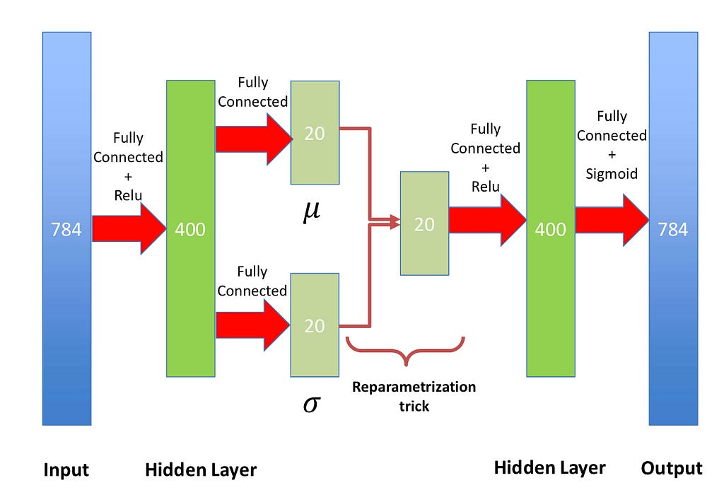
While typical autoencoders are deterministic, VAEs are probabilistic models due to modeling the latent space as a probability distribution. VAEs are unsupervised models that encode input data x into a latent representation z and reconstruct the input from this latent space. They technically don’t need to be implemented with neural networks and can be constructed from generative probability models. However, in our current state of deep learning, most are typically implemented with neural networks.
Example VAE framework with reparameterization trick. Source: Author
Explained briefly, the reparameterization trick is used since we can’t backpropagate on the probabilistic distribution of the latent space, but we need to update our encoding distribution. Therefore, we define a differentiable and invertible function so that we can differentiate with respect to lambda and x while still keeping a probabilistic element.
Reparameterization trick for z. Source: Author
VAEs are trained using an ELBO loss consisting of a reconstruction term and a Kullback-Leibler Divergence (KLD) of the encoding model to the prior distribution.
Loss function for VAE with KLD term on left and reconstruction term on righ [1]
Adding a Conditional Input to VAE
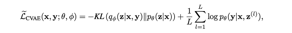
CVAEs extend VAEs by incorporating additional information such as class labels as conditional variables. This conditioning enables CVAEs to produce controlled generations. The conditional input feature can be added at differing points in the architecture, but it is commonly inserted with the encoder and the decoder. The loss function with the conditional input is an adaptation of the ELBO loss in the traditional VAE.
Loss function for VAE with KLD term on left and reconstruction term on right [2]
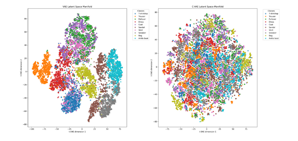
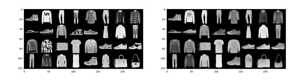
To illustrate the difference between a VAE and CVAE, both networks were trained on Fashion-MNIST using a convolutional encoder and decoder architecture. A tSNE of the latent space of each network is shown.
Latent space manifold of VAE (left) and CVAE (right). Source: Author
The vanilla VAE shows distinct clusters while the CVAE has a more homogeneous distribution. Vanilla VAE encodes class and class variation into the latent space since there is no provided conditional signal. However, the CVAE does not need to learn class distinction and the latent space can focus on the variation within classes. Therefore, a CVAE can potentially learn more information as it does not rely on having to learn basic class conditioning.
Model Architecture for CVAEs
Two model architectures were created to test image generation. The first architecture was a convolutional CVAE with a concatenating conditional approach. All networks were built for Fashion-MNIST images of size 28×28 (784 total pixels).
def decode(self, z, c): c = self.label_embedding(c) # Concatenate condition with latent vector z = torch.cat([z, c], dim=1) z = self.decoder_input(z) z = z.view(-1, 128, 4, 4) return self.decoder(z)
def forward(self, x, c): mu, log_var = self.encode(x, c) z = self.reparameterize(mu, log_var) return self.decode(z, c), mu, log_var
The CVAE encoder consists of 3 convolutional layers each followed by a ReLU non-linearity. The output of the encoder is then flattened. The class number is then passed through an embedding layer and added to the encoder output. The reparameterization trick is then used with 2 linear layers to obtain a μ and σ in the latent space. Once sampled, the output of the reparameterized latent space is passed to the decoder now concatenated with the class number embedding layer output. The decoder consists of 3 transposed convolutional layers. The first two contain a ReLU non-linearity with the last layer containing a sigmoid non-linearity. The output of the decoder is a 28×28 generated image.
The other model architecture follows the same approach but with adding the conditional input instead of concatenating. A major question was if adding or concatenating will lead to better reconstruction or generation results.
def decode(self, z, c): # Add condition to latent vector c = self.decoder_label_embedding(c) z = z + c z = self.decoder_input(z) z = z.view(-1, 128, 4, 4) return self.decoder(z)
def forward(self, x, c): mu, log_var = self.encode(x, c) z = self.reparameterize(mu, log_var) return self.decode(z, c), mu, log_var
The same loss function is used for all CVAEs from the equation shown above.
def loss_function(recon_x, x, mu, logvar):
    """Computes the loss = -ELBO = Negative Log-Likelihood + KL Divergence.
        Args:
        recon_x: Decoder output.
        x: Ground truth.
        mu: Mean of Z
        logvar: Log-Variance of Z
    """
    BCE = F.binary_cross_entropy(recon_x, x, reduction='sum')
    KLD = -0.5 * torch.sum(1 + logvar - mu.pow(2) - logvar.exp())
    return BCE + KLD
In order to assess model-generated images, 3 quantitative metrics are commonly used. Mean Squared Error (MSE) was calculated by summing the squares of the difference between the generated image and a ground truth image pixel-wise. Structural Similarity Index Measure (SSIM) is a metric that evaluates image quality by comparing two images based on structural information, luminance, and contrast [3]. SSIM can be used to compare images of any size while MSE is relative to pixel size. SSIM score ranges from -1 to 1, where 1 indicates identical images. Frechet inception distance (FID) is a metric for quantifying the realism and diversity of images generated. As FID is a distance measure, lower scores are indicative of a better reconstruction of a set of images.
Short Text to Image from Fashion-MNIST
Before scaling up to full text to image, CVAEs image reconstruction and generation on Fashion-MNIST. Fashion-MNIST is an MNIST-like dataset consisting of a training set of 60,000 examples and a test set of 10,000 examples. Each example is a 28×28 grayscale image, associated with a label from 10 classes [4].
Preprocessing functions were created to extract the relevant key word containing the class name from the input short-text regular expression matching. Extra descriptors (synonyms) were used for most classes to account for similar fashion items included in each class (e.g. Coat & Jacket).
def class_embedding(input_str, classes): for key in list(classes.keys()): template = f'(?i)\b{key}\b' output = re.search(template, input_str) if output: return classes[key] return -1
The class name was then converted to its class number and used as the conditional input to the CVAE along. In order to generate an image, the class label extracted from the short text description is passed into the decoder with random samples from a Gaussian distribution to input the variable from the latent space.
Before testing generation, image reconstruction is tested to ensure the functionality of the CVAE. Due to creating a convolutional network with 28×28 images, the network can be trained in less than an hour with less than 100 epochs.
CVAE reconstruction results with ground truth (left) and model output (right). Source: Author
Reconstructions contain the general shape of the ground truth images, but sharp, high frequency features are missing from the image. Any text or intricate design patterns are blurred in the model output. Inputting any short text containing a class of Fashion-MNIST gives generated outputs resembling reconstructed images.
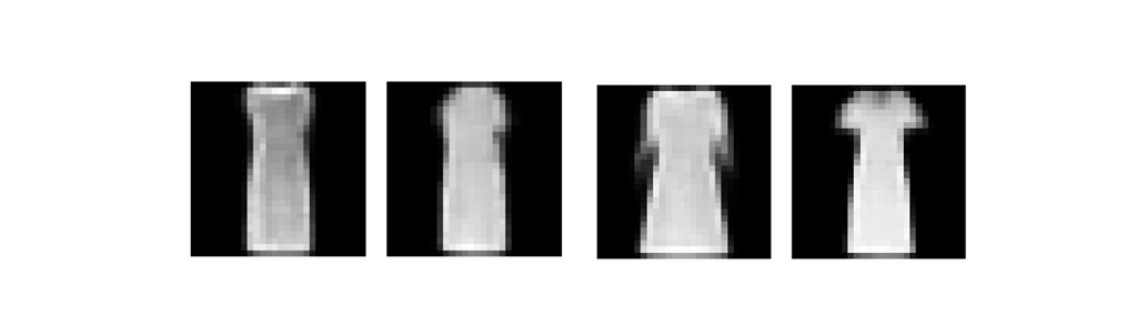
Generated images “dress” from CVAE Fashion-MNIST. Source: Author
The generated images have an MSE of 11 and a SSIM of 0.76. These constitute good generations signifying that in simple, small images, CVAEs can generate quality images. GANs and DDPMs will produce higher quality images with complex features, but CVAEs can handle simple cases.
Long Text to Image using CLIP and COCO
When scaling up to image generation to text of any length, more robust methods would be needed besides regular expression matching. To do this, Open AI’s CLIP is used to convert text into a high dimensional embedding vector. The embedding model is used in its ViT-B/32 configuration, which outputs embeddings of length 512. A limitation of the CLIP model is that it has a maximum token length of 77, with studies showing an even smaller effective length of 20 [5]. Thus, in instances where the input text contains multiple sentences, the text is split up by sentence and passed through the CLIP encoder. The resulting embeddings are averaged together to create the final output embedding.
A long text model requires far more complicated training data than Fashion-MNIST, so COCO dataset was used. COCO dataset has annotations (that are not completely robust but that will be discussed later) that can be passed into CLIP to get embeddings. However, COCO images are of size 640×480, meaning that even with cropping transforms, a larger network is needed. Adding and concatenating conditional inputs architectures are both tested for long text to image generation, but the concatenating approach is shown here:
class cVAE(nn.Module): def __init__(self, latent_dim=128): super().__init__()
device = torch.device("cuda" if torch.cuda.is_available() else "cpu")
self.clip_model, _ = clip.load("ViT-B/32", device=device) self.clip_model.eval() for param in self.clip_model.parameters(): param.requires_grad = False
def decode(self, z, c): z = torch.cat([z, c], dim=1) z = self.decoder_input(z) z = z.view(-1, 512, 4, 4) return self.decoder(z)
def forward(self, x, c): mu, log_var = self.encode(x, c) z = self.reparameterize(mu, log_var) return self.decode(z, c), mu, log_var
Another major point of investigation was image generation and reconstruction on images of different sizes. Specifically, modifying COCO images to be of size 64×64, 128×128, and 256×256. After training the network, reconstruction results should first be tested.
CVAE reconstruction on COCO with different image sizes. Source: Author
All image sizes lead to reconstructed background with some feature outlines and correct colors. However, as image size increases, more features are able to be recovered. This makes sense as although it will take a lot longer to train a model with a larger image size, there is more information that can be captured and learned by the model.
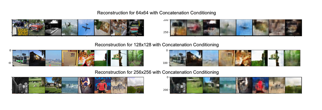
With image generation, it is extremely difficult to generate high quality images. Most images have backgrounds to some degree and blurred features in the image. This would be expected for image generation from a CVAE. This occurs in both concatenation and addition for the conditional input, but the concatenated approach performs better. This is likely because concatenated conditional inputs will not interfere with important features and ensures information is preserved distinctly. Conditions can be ignored if they are irrelevant. However, additive conditional inputs can interfere with existing features and completely mess up the network when updating weights during backpropagation.
Generated images by CVAE on COCO. Source: Author
All of the COCO generated images have a far lower SSIM of about 0.4 compared to the SSIM on Fashion-MNIST. MSE is proportional to image size, so it is difficult to quanity differences. FID for COCO image generations are in the 200s for further proof that COCO CVAE generated images are not robust.
Limitations of CVAEs for Image Generation
The biggest limitation in trying to use CVAEs for image generation is, well, the CVAE. The amount of information that can be contained and reconstructed/generated is extremely dependent on the size of the latent space. A latent space that is too small won’t capture any meaningful information and is proportional to the size of the output image. A 28×28 image needs a far smaller latent space than a 64×64 image (as it proportionally squares from image size). However, a latent space bigger than the actual image adds unnecessary info and at that point just create a 1-to-1 mapping. For the COCO dataset, a latent space of at least 512 is needed to capture some features. And while CVAEs are generative models, a convolutional encoder and decoder is a rather rudimentary network. The training style of a GAN or the complex denoising process of a DDPM allows for far more complicated image generation.
Another major limitation in image generation is the dataset trained on. Although the COCO dataset has annotations, the annotations are not extensively detailed. In order to train complex generative models, a different dataset should be used for training. COCO does not provide locations or excess information for background details. A complex feature vector from the CLIP encoder can’t be effectively utilized to a CVAE on COCO.
Although CVAEs and image generation on COCO have their limitations, it creates a workable image generation model. More code and details can be provided just reach out!
The 80/20 problem of generative AI — a UX research insight
When an LLM solves a task 80% correctly, that often only amounts to 20% of the user value.
The Pareto principle says if you solve a problem 20% through, you get 80% of the value. The opposite seems to be true for generative AI.
About the author: Zsombor Varnagy-Toth is a Sr UX Researcher at SAP with background in machine learning and cognitive science. Working with qualitative and quantitative data for product development.
I first realized this as I studied professionals writing marketing copy using LLMs. I observed that when these professionals start using LLMs, their enthusiasm quickly fades away, and most return to their old way of manually writing content.
This was an utterly surprising research finding because these professionals acknowledged that the AI-generated content was not bad. In fact, they found it unexpectedly good, say 80% good. But if that’s so, why do they still fall back on creating the content manually? Why not take the 80% good AI-generated content and just add that last 20% manually?
Here is the intuitive explanation:
If you have a mediocre poem, you can’t just turn it into a great poem by replacing a few words here and there.
Say, you have a house that is 80% well built. It’s more or less OK, but the walls are not straight, and the foundations are weak. You can’t fix that with some additional work. You have to tear it down and start building it from the ground up.
We investigated this phenomenon further and identified its root. For these marketing professionals if a piece of copy is only 80% good, there is no individual piece in the text they could swap that would make it 100%. For that, the whole copy needs to be reworked, paragraph by paragraph, sentence by sentence. Thus, going from AI’s 80% to 100% takes almost as much effort as going from 0% to 100% manually.
Now, this has an interesting implication. For such tasks, the value of LLMs is “all or nothing.” It either does an excellent job or it’s useless. There is nothing in between.
We looked at a few different types of user tasks and figured that this reverse Pareto principle affects a specific class of tasks.
Not easily decomposable and
Large task size and
100% quality is expected
If one of these conditions are not met, the reverse Pareto effect doesn’t apply.
Writing code, for example, is more composable than writing prose. Code has its individual parts: commands and functions that can be singled out and fixed independently. If AI takes the code to 80%, it really only takes about 20% extra effort to get to the 100% result.
As for the task size, LLMs have great utility in writing short copy, such as social posts. The LLM-generated short content is still “all or nothing” — it’s either good or worthless. However, because of the brevity of these pieces of copy, one can generate ten at a time and spot the best one in seconds. In other words, users don’t need to tackle the 80% to 100% problem — they just pick the variant that came out 100% in the first place.
As for quality, there are those use cases when professional grade quality is not a requirement. For example, a content factory may be satisfied with 80% quality articles.
What does this mean for product development?
If you are building an LLM-powered product that deals with large tasks that are hard to decompose but the user is expected to produce 100% quality, you must build something around the LLM that turns its 80% performance into 100%. It can be a sophisticated prompting approach on the backend, an additional fine-tuned layer, or a cognitive architecture of various tools and agents that work together to iron out the output. Whatever this wrapper does, that’s what gives 80% of the customer value. That’s where the treasure is buried, the LLM only contributes 20%.
This conclusion is in line with Sequoia Capital’s Sonya Huang’s and Pat Grady’s assertion that the next wave of value in the AI space will be created by these “last-mile application providers” — the wrapper companies that figure out how to jump that last mile that creates 80% of the value.
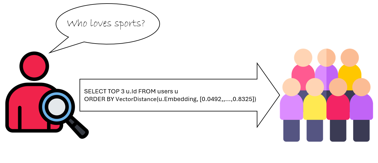
LEC surpasses best in class models, like GPT-4o, by combining the efficiency of a ML classifier with the language understanding of an LLM
Imagine sitting in a boardroom, discussing the most transformative technology of our time — artificial intelligence — and realizing we’re riding a rocket with no reliable safety belt. The Bletchley Declaration, unveiled during the AI Safety Summit hosted by the UK government and backed by 29 countries, captures this sentiment perfectly [1]:
“There is potential for serious, even catastrophic, harm, either deliberate or unintentional, stemming from the most significant capabilities of these AI models”.
Source: Dalle3
However, existing AI safety approaches force organizations into an un-winnable trade-off between cost, speed, and accuracy. Traditional machine learning classifiers struggle to capture the subtleties of natural language and LLM’s, while powerful, introduce significant computational overhead — requiring additional model calls that escalate costs for each AI safety check.
Image by : Sandi Besen, Tula Masterman, Mason Sawtell, Jim Brown
We prove LEC combines the computational efficiency of a machine learning classifier with the sophisticated language understanding of an LLM — so you don’t have to choose between cost, speed, and accuracy. LEC surpasses best in class models like GPT-4o and models specifically trained for identifying unsafe content and prompt injections. What’s better yet, we believe LEC can be modified to tackle non AI safety related text classification tasks like sentiment analysis, intent classification, product categorization, and more.
The implications are profound. Whether you’re a technology leader navigating the complex terrain of AI safety, a product manager mitigating potential risks, or an executive charting a responsible innovation strategy, our approach offers a scalable and adaptable solution.
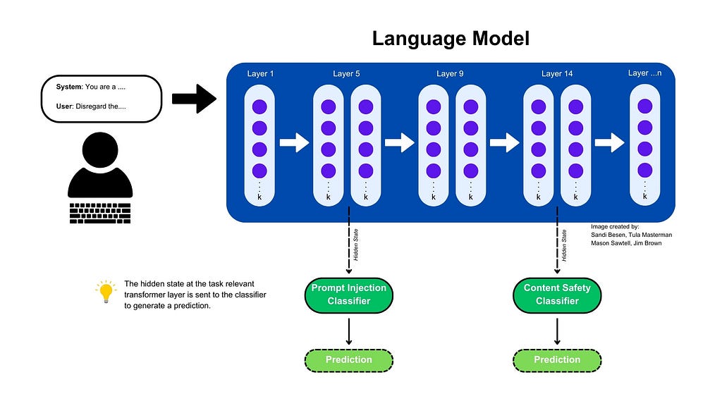
Figure 1: An example of an adapted model inference pipeline to include LEC Classifiers. Image by : Sandi Besen, Tula Masterman, Mason Sawtell, Jim Brown
Responsible AI has become a critical priority for technology leaders across the ecosystem — from model developers like Anthropic, OpenAI, Meta, Google, and IBM to enterprise consulting firms and AI service providers. As AI adoption accelerates, its importance becomes even more pronounced.
Our research specifically targets two pivotal challenges in AI safety — content safety and prompt injection detection. Content safety refers to the process of identifying and preventing the generation of harmful, inappropriate, or potentially dangerous content that could pose risks to users or violate ethical guidelines. Prompt injection involves detecting attempts to manipulate AI systems by crafting input prompts designed to bypass safety mechanisms or coerce the model into producing unethical outputs.
To advance the field of ethical AI, we applied LEC’s capabilities to real-world responsible AI use cases. Our hope is that this methodology will be adopted widely, helping to make every AI system less vulnerable to exploitation.
Using LEC for Content Safety Tasks
We curated a content safety dataset of 5,000 examples to test LEC on both binary (2 categories) and multi-class (>2 categories) classification. We used the SALAD Data dataset from OpenSafetyLab [3] to represent unsafe content and the “LMSYS-Chat-1M” dataset from LMSYS, to represent safe content [4].
For binary classification the content is either “safe” or “unsafe”. For multi-class classification, content is either categorized as “safe” or assigned to a specific specific “unsafe” category.
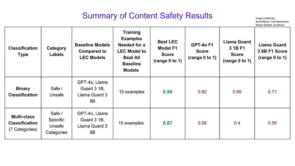
We compared model’s trained using LEC to GPT-4o (widely recognized as an industry leader), Llama Guard 3 1B and Llama Guard 3 8B (special purpose models specifically trained to tackle content safety tasks). We found that the models using LEC outperformed all models we compared them to using as few as 20 training examples for binary classification and 50 training examples for multi-class classification.
The highest performing LEC model achieved a weighted F1 score (measures how well a system balances making correct predictions while minimizing mistakes) of .96 of a maximum score of 1 on the binary classification task compared to GPT-4o’s score of 0.82 or LlamaGuard 8B’s score of 0.71.
This means that with as few as 15 examples, using LEC you can train a model to outperform industry leaders in identifying safe or unsafe content at a fraction of the computational cost.
Summary of Content safety Results. Image by : Sandi Besen, Tula Masterman, Mason Sawtell, Jim Brown
Using LEC for Identifying Prompt Injections
We curated a prompt injection dataset using the SPML Chatbot Prompt Injection Dataset. We chose the SPML dataset because of its diversity and complexity in representing real-world chat bot scenarios. This dataset contained pairs of system and user prompts to identify user prompts that attempt to defy or manipulate the system prompt. This is especially relevant for businesses deploying public facing chatbots that are only meant to answer questions about specific domains.
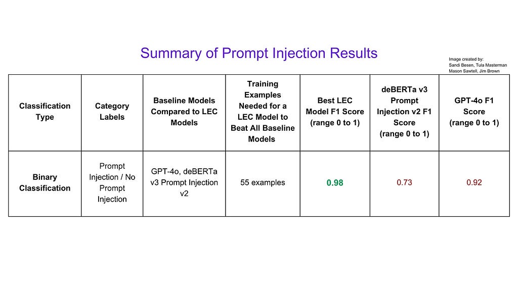
We compared model’s trained using LEC to GPT-4o (an industry leader) and deBERTa v3 Prompt Injection v2 (a model specifically trained to identify prompt injections). We found that the models using LEC outperformed both GPT-4o using 55 training examples and the the special purpose model using as few as 5 training examples.
The highest performing LEC model achieved a weighted F1 score of .98 of a maximum score of 1 compared to GPT-4o’s score of 0.92 or deBERTa v2 Prompt Injection v2’s score of 0.73.
This means that with as few as 5 examples, using LEC you can train a model to outperform industry leaders in identifying prompt injection attacks.
Summary of Prompt Injection Results. Image by : Sandi Besen, Tula Masterman, Mason Sawtell, Jim Brown
Full results and experimentation implementation details can be found in the Arxiv preprint.
How Your Business Can Benefit From using LEC
As organizations increasingly integrate AI into their operations, ensuring the safety and integrity of AI-driven interactions has become mission-critical. LEC provides a robust and flexible way to ensure that potentially unsafe information is being detected — resulting in reduce operational risk and increased end user trust. There are several ways that a LEC models can be incorporated into your AI Safety Toolkit to prevent unwanted vulnerabilities when using your AI tools including during LM inference, before/after LM inference, and even in multi-agent scenarios.
During LM Inference
If you are using an open-source model or have access to the inner workings of the closed-source model, you can use LEC as part of your inference pipeline for AI safety in near real time. This means that if any safety concerns arise while information is traveling through the language model, generation of any output can be halted. An example of what this might look like can be seen in figure 1.
Before / After LM Inference
If you don’t have access to the inner workings of the language model or want to check for safety concerns as a separate task you can use a LEC model before or after calling a language model. This makes LEC compatible with closed source models like the Claude and GPT families.
Building a LEC Classifier into your deployment pipeline can save you from passing potentially harmful content into your LM and/or check for harmful content before an output is returned to the user.
Using LEC Classifiers with Agents
Agentic AI systems can amplify any existing unintended actions, leading to a compounding effect of unintended consequences. LEC Classifiers can be used at different times throughout an agentic scenario to can safeguard the agent from either receiving or producing harmful outputs. For instance, by including LEC models into your agentic architecture you can:
Check that the request is ok to start working on
Ensure an invoked tool call does not violate any AI safety guidelines (e.g., generating inappropriate search topics for a keyword search)
Make sure information returned to an agent is not harmful (e.g., results returned from RAG search or google search are “safe”)
Validating the final response of an agent before passing it back to the user
How to Implement LEC Based on Language Model Access
Enterprises with access to the internal workings of models can integrate LEC directly within the inference pipeline, enabling continuous safety monitoring throughout the AI’s content generation process. When using closed-source models via API (as is the case with GPT-4), businesses do not have direct access to the underlying information needed to train a LEC model. In this scenario, LEC can be applied before and/or after model calls. For example, before an API call, the input can be screened for unsafe content. Post-call, the output can be validated to ensure it aligns with business safety protocols.
No matter which way you choose to implement LEC, using its powerful abilities provides you with superior content safety and prompt injection protection than existing techniques at a fraction of the time and cost.
Conclusion
Layer Enhanced Classification (LEC) is the safety belt for that AI rocket ship we’re on.
The value proposition is clear: LEC’s AI Safety models can mitigate regulatory risk, help ensure brand protection, and enhance user trust in AI-driven interactions. It signals a new era of AI development where accuracy, speed, and cost aren’t competing priorities and AI safety measures can be addressed both at inference time, before inference time, or after inference time.
In our content safety experiments, the highest performing LEC model achieved a weighted F1 score of 0.96 out of 1 on binary classification, significantly outperforming GPT-4o’s score of 0.82 and LlamaGuard 8B’s score of 0.71 — and this was accomplished with as few as 15 training examples. Similarly, in prompt injection detection, our top LEC model reached a weighted F1 score of 0.98, compared to GPT-4o’s 0.92 and deBERTa v2 Prompt Injection v2’s 0.73, and it was achieved with just 55 training examples. These results not only demonstrate superior performance, but also highlight LEC’s remarkable ability to achieve high accuracy with minimal training data.
Although our work focused on using LEC Models for AI safety use cases, we anticipate that our approach can be used for a wider variety of text classification tasks. We encourage the research community to use our work as a stepping stone for exploring what else can be achieved — further open new pathways for more intelligent, safer, and more trustworthy AI systems.
Note: The opinions expressed both in this article and paper are solely those of the authors and do not necessarily reflect the views or policies of their respective employers.
Interested in connecting? Drop me a DM on Linkedin! I‘m always eager to engage in food for thought and iterate on my work.
Large language models are fantastic tools for unstructured text, but what if your text doesn’t fit in the context window? Bazaarvoice faced exactly this challenge when building our AI Review Summaries feature: millions of user reviews simply won’t fit into the context window of even newer LLMs and, even if they did, it would be prohibitively expensive.
In this post, I share how Bazaarvoice tackled this problem by compressing the input text without loss of semantics. Specifically, we use a multi-pass hierarchical clustering approach that lets us explicitly adjust the level of detail we want to lose in exchange for compression, regardless of the embedding model chosen. The final technique made our Review Summaries feature financially feasible and set us up to continue to scale our business in the future.
The Problem
Bazaarvoice has been collecting user-generated product reviews for nearly 20 years so we have a lot of data. These product reviews are completely unstructured, varying in length and content. Large language models are excellent tools for unstructured text: they can handle unstructured data and identify relevant pieces of information amongst distractors.
LLMs have their limitations, however, and one such limitation is the context window: how many tokens (roughly the number of words) can be put into the network at once. State-of-the-art large language models, such as Athropic’s Claude version 3, have extremely large context windows of up to 200,000 tokens. This means you can fit small novels into them, but the internet is still a vast, every-growing collection of data, and our user-generated product reviews are no different.
We hit the context window limit while building our Review Summaries feature that summarizes all of the reviews of a specific product on our clients website. Over the past 20 years, however, many products have garnered thousands of reviews that quickly overloaded the LLM context window. In fact, we even have products with millions of reviews that would require immense re-engineering of LLMs to be able to process in one prompt.
Even if it was technically feasible, the costs would be quite prohibitive. All LLM providers charge based on the number of input and output tokens. As you approach the context window limits for each product, of which we have millions, we can quickly run up cloud hosting bills in excess of six figures.
Our Approach
To ship Review Summaries despite these technical, and financial, limitations, we focused on a rather simple insight into our data: Many reviews say the same thing. In fact, the whole idea of a summary relies on this: review summaries capture the recurring insights, themes, and sentiments of the reviewers. We realized that we can capitalize on this data duplication to reduce the amount of text we need to send to the LLM, saving us from hitting the context window limit and reducing the operating cost of our system.
To achieve this, we needed to identify segments of text that say the same thing. Such a task is easier said than done: often people use different words or phrases to express the same thing.
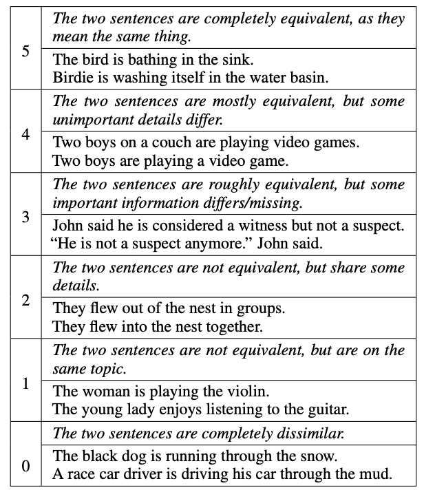
Fortunately, the task of identifying if text is semantically similar has been an active area of research in the natural language processing field. The work by Agirre et. al. 2013 (SEM 2013 shared task: Semantic Textual Similarity. In Second Joint Conference on Lexical and Computational Semantics) even published a human-labeled data of semantically similar sentences known as the STS Benchmark. In it, they ask humans to indicate if textual sentences are semantically similar or dissimilar on a scale of 1–5, as illustrated in the table below (from Cer et. al., SemEval-2017 Task 1: Semantic Textual Similarity Multilingual and Crosslingual Focused Evaluation):
The STSBenchmark dataset is often used to evaluate how well a text embedding model can associate semantically similar sentences in its high-dimensional space. Specifically, Pearson’s correlation is used to measure how well the embedding model represents the human judgements.
Thus, we can use such an embedding model to identify semantically similar phrases from product reviews, and then remove repeated phrases before sending them to the LLM.
Our approach is as follows:
First, product reviews are segmented the into sentences.
An embedding vector is computed for each sentence using a network that performs well on the STS benchmark
Agglomerative clustering is used on all embedding vectors for each product.
An example sentence — the one closest to the cluster centroid — is retained from each cluster to send to the LLM, and other sentences within each cluster are dropped.
Any small clusters are considered outliers, and those are randomly sampled for inclusion in the LLM.
The number of sentences each cluster represents is included in the LLM prompt to ensure the weight of each sentiment is considered.
This may seem straightforward when written in a bulleted list, but there were some devils in the details we had to sort out before we could trust this approach.
Embedding Model Evaluation
First, we had to ensure the model we used effectively embedded text in a space where semantically similar sentences are close, and semantically dissimilar ones are far away. To do this, we simply used the STS benchmark dataset and computed the Pearson correlation for the models we desired to consider. We use AWS as a cloud provider, so naturally we wanted to evaluate their Titan Text Embedding models.
Below is a table showing the Pearson’s correlation on the STS Benchmark for different Titan Embedding models:
So AWS’s embedding models are quite good at embedding semantically similar sentences. This was great news for us — we can use these models off the shelf and their cost is extremely low.
Semantically Similar Clustering
The next challenge we faced was: how can we enforce semantic similarity during clustering? Ideally, no cluster would have two sentences whose semantic similarity is less than humans can accept — a score of 4 in the table above. Those scores, however, do not directly translate to the embedding distances, which is what is needed for agglomerative clustering thresholds.
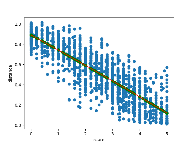
To deal with this issue, we again turned to the STS benchmark dataset. We computed the distances for all pairs in the training dataset, and fit a polynomial from the scores to the distance thresholds.
Image by author
This polynomial lets us compute the distance threshold needed to meet any semantic similarity target. For Review Summaries, we selected a score of 3.5, so nearly all clusters contain sentences that are “roughly” to “mostly” equivalent or more.
It’s worth noting that this can be done on any embedding network. This lets us experiment with different embedding networks as they become available, and quickly swap them out should we desire without worrying that the clusters will have semantically dissimilar sentences.
Multi-Pass Clustering
Up to this point, we knew we could trust our semantic compression, but it wasn’t clear how much compression we could get from our data. As expected, the amount of compression varied across different products, clients, and industries.
Without loss of semantic information, i.e., a hard threshold of 4, we only achieved a compression ratio of 1.18 (i.e., a space savings of 15%).
Clearly lossless compression wasn’t going to be enough to make this feature financially viable.
Our distance selection approach discussed above, however, provided an interesting possibility here: we can slowly increase the amount of information loss by repeatedly running the clustering at lower thresholds for remaining data.
The approach is as follows:
Run the clustering with a threshold selected from score = 4. This is considered lossless.
Select any outlying clusters, i.e., those with only a few vectors. These are considered “not compressed” and used for the next phase. We chose to re-run clustering on any clusters with size less than 10.
Run clustering again with a threshold selected from score = 3. This is not lossless, but not so bad.
Select any clusters with size less than 10.
Repeat as desired, continuously decreasing the score threshold.
So, at each pass of the clustering, we’re sacrificing more information loss, but getting more compression and not muddying the lossless representative phrases we selected during the first pass.
In addition, such an approach is extremely useful not only for Review Summaries, where we want a high level of semantic similarity at the cost of less compression, but for other use cases where we may care less about semantic information loss but desire to spend less on prompt inputs.
In practice, there are still a significantly large number of clusters with only a single vector in them even after dropping the score threshold a number of times. These are considered outliers, and are randomly sampled for inclusion in the final prompt. We select the sample size to ensure the final prompt has 25,000 tokens, but no more.
Ensuring Authenticity
The multi-pass clustering and random outlier sampling permits semantic information loss in exchange for a smaller context window to send to the LLM. This raises the question: how good are our summaries?
At Bazaarvoice, we know authenticity is a requirement for consumer trust, and our Review Summaries must stay authentic to truly represent all voices captured in the reviews. Any lossy compression approach runs the risk of mis-representing or excluding the consumers who took time to author a review.
To ensure our compression technique was valid, we measured this directly. Specifically, for each product, we sampled a number of reviews, and then used LLM Evals to identify if the summary was representative of and relevant to each review. This gives us a hard metric to evaluate and balance our compression against.
Results
Over the past 20 years, we have collected nearly a billion user-generated reviews and needed to generate summaries for tens of millions of products. Many of these products have thousands of reviews, and some up to millions, that would exhaust the context windows of LLMs and run the price up considerably.
Using our approach above, however, we reduced the input text size by 97.7% (a compression ratio of 42), letting us scale this solution for all products and any amount of review volume in the future. In addition, the cost of generating summaries for all of our billion-scale dataset reduced 82.4%. This includes the cost of embedding the sentence data and storing them in a database.
The Case for Predicting Full Probability Distributions in Decision-Making
Some people like hot coffee, some people like iced coffee, but no one likes lukewarm coffee. Yet, a simple model trained on coffee temperatures might predict that the next coffee served should be… lukewarm. This illustrates a fundamental problem in predictive modeling: focusing on single point estimates (e.g., averages) can lead us to meaningless or even misleading conclusions.
In “The Crystal Ball Fallacy” (Merckel, 2024b), we explored how even a perfect predictive model does not tell us exactly what will happen — it tells us what could happen and how likely each outcome is. In other words, it reveals the true distribution of a random variable. While such a perfect model remains hypothetical, real-world models should still strive to approximate these true distributions.
Yet many predictive models used in the corporate world do something quite different: they focus solely on point estimates — typically the mean or the mode — rather than attempting to capture the full range of possibilities. This is not just a matter of how the predictions are used; this limitation is inherent in the design of many conventional machine learning algorithms. Random forests, generalized linear models (GLM), artificial neural networks (ANNs), and gradient boosting machines, among others, are all designed to predict the expected value (mean) of a distribution when used for regression tasks. In classification problems, while logistic regression and other GLMs naturally attempt to estimate probabilities of class membership, tree-based methods like random forests and gradient boosting produce raw scores that would require additional calibration steps (like isotonic regression or Platt scaling) to be transformed into meaningful probabilities. Yet in practice, this calibration is rarely performed, and even when uncertainty information is available (i.e., the probabilities), it is typically discarded in favor of the single most likely class, i.e., the mode.
This oversimplification is sometimes not just inadequate; it can lead to fundamentally wrong conclusions, much like our lukewarm coffee predictor. A stark example is the Gaussian copula formula used to price collateralized debt obligations (CDOs) before the 2008 financial crisis. By reducing the complex relationships between mortgage defaults to a single correlation number, among other issues, this model catastrophically underestimated the possibility of simultaneous defaults (MacKenzie & Spears, 2014). This systematic underestimation of extreme risks is so pervasive that some investment funds, like Universa Investments advised by Nassim Taleb, incorporate strategies to capitalize on it. They recognize that markets consistently undervalue the probability and impact of extreme events (Patterson, 2023). When we reduce a complex distribution of possible outcomes to a single number, we lose critical information about uncertainty, risk, and potential extreme events that could drastically impact decision-making.
On the other hand, some quantitative trading firms have built their success partly by properly modeling these complex distributions. When asked about Renaissance Technologies’ approach — whose Medallion fund purportedly achieved returns of 66% annually before fees from 1988 to 2018 (Zuckerman, 2019) — founder Jim Simons emphasized that they carefully consider that market risk “is typically not a normal distribution, the tails of a distribution are heavier and the inside is not as heavy” (Simons, 2013, 47:41), highlighting the critical importance of looking beyond simple averages.
Why, then, do we persist in using point estimates despite their clear limitations? The reasons may be both practical and cultural. Predicting distributions is technically more challenging than predicting single values, requiring more sophisticated models and greater computational resources. But more fundamentally, most business processes and tools are simply not designed to handle distributional thinking. You cannot put a probability distribution in a spreadsheet cell, and many decision-making frameworks demand concrete numbers rather than ranges of possibilities. Moreover, as Kahneman (2011) notes in his analysis of human decision-making, we are naturally inclined to think in terms of specific scenarios rather than statistical distributions — our intuitive thinking prefers simple, concrete answers over probabilistic ones.
Let us examine actual housing market data to illustrate potential issues with single-point valuation and possible modeling techniques to capture the full distribution of possible values.
A Deep Dive into Property Pricing
In this section, we use the French Real Estate Transactions (DVF) dataset provided by the French government (gouv.fr, 2024), which contains comprehensive records of property transactions across France. For this analysis, we focus on sale prices, property surface areas, and the number of rooms for the years ranging from 2014 to 2024. Notably, we exclude critical information such as geolocation, as our aim is not to predict house prices but to demonstrate the benefits of predicting distributions over relying solely on single-point estimates.
First, we will go through a fictional — yet most likely à clef — case study where a common machine learning technique is put into action for planning an ambitious real estate operation. Subsequently, we will adopt a critical stance on this case and offer alternatives that many may prefer in order to be better prepared for pulling off the trade.
Case Study: The Homer & Lisa Reliance on AI for Real Estate Trading
Homer and Lisa live in Paris. They expect the family to grow and envisage to sell their two-room flat to fund the acquisition of a four-room property. Given the operational and maintenance costs, and the capacity of their newly acquired state-of-the-art Roomba with all options, they reckoned that 90m² is the perfect surface area for them. They want to estimate how much they need to save/borrow to complement the proceeds from the sale. Homer followed a MOOC on machine learning just before graduating in advanced French literature last year, and immediately found — thanks to his network — a data scientist role at a large reputable traditional firm that was heavily investing in expanding (admittedly from scratch, really) its AI capacity to avoid missing out. Now a Principal Senior Lead Data Scientist, after almost a year of experience, he knows quite a bit! (He even works for a zoo as a side hustle, where his performance has not remained unnoticed — Merckel, 2024a.)
Following some googling, he found the real estate dataset freely provided by the government. He did a bit of cleaning, filtering, and aggregating to obtain the perfect ingredients for his ordinary least squares model (OLS for those in the know). He can now confidently predict prices, in the Paris area, from both the number of rooms and the surface. Their 2-room, 40m², flat is worth 365,116€. And a 4-room, 90m², reaches 804,911€. That is a no-brainer; they must calculate the difference, i.e., 439,795€.
Homer & Lisa: The Ones Playing Darts… Unknowingly!
Do Homer and Lisa need to save/borrow 439,795€? The model certainly suggests so. But is that so?
Perhaps Homer, if only he knew, could have provided confidence intervals? Using OLS, confidence intervals can either be estimated empirically via bootstrapping or analytically using standard error-based methods.
Besides, even before that, he could have looked at the price distribution, and realized the default OLS methods may not be the best choice…
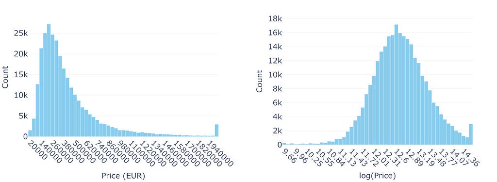
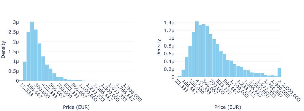
Figure 1: Real Estate Prices Near Paris (2014–2024): The left plot illustrates the distribution of real estate prices within a 7km radius of central Paris. The right plot shows the distribution of the natural logarithm of those prices. In both histograms, the final bar represents the cumulative count of properties priced above 2,000,000€ (or log(2,000,000) in the logarithmic scale). Image by the author.
The right-skewed shape with a long tail is hard to miss. For predictive modeling (as opposed to, e.g., explanatory modeling), the primary concern with OLS is not necessarily the normality (and homoscedasticity) of errors but the potential for extreme values in the long tail to disproportionately influence the model — OLS minimizes squared errors, making it sensitive to extreme observations, particularly those that deviate significantly from the Gaussian distribution assumed for the errors.
A Generalized Linear Model (GLM) extends the linear model framework by directly specifying a distribution for the response variable (from the exponential family) and using a “link function” to connect the linear predictor to the mean of that distribution. While linear models assume normally distributed errors and estimate the expected response E(Y) directly through a linear predictor, GLMs allow for different response distributions and transform the relationship between the linear predictor and E(Y) through the link function.
Let us revisit Homer and Lisa’s situation using a simpler but related approach. Rather than implementing a GLM, we can transform the data by taking the natural logarithm of prices before applying a linear model. This implies we are modeling prices as following a log-normal distribution (Figure 1 presents the distribution of prices and the log version). When transforming predictions back to the original scale, we need to account for the bias introduced by the log transformation using Duan’s smearing estimator (Duan, 1983). Using this bias-corrected log-normal model and fitting it on properties around Paris, their current 2-room, 40m² flat is estimated at 337,844€, while their target 4-room, 90m² property would cost around 751,884€, hence a need for an additional 414,040€.
The log-normal model with smearing correction is particularly suitable for this context because it not only reflects multiplicative relationships, such as price increasing proportionally (by a factor) rather than by a fixed amount when the number of rooms or surface area increases, but also properly accounts for the retransformation bias that would otherwise lead to systematic underestimation of prices.
To better understand the uncertainty in these predictions, we can examine their confidence intervals. The 95% bootstrap confidence interval [400,740€ — 418,618€] for the mean price difference means that if we were to repeat this sampling process many times, about 95% of such intervals would contain the true mean price difference. This interval is more reliable in this context than the standard error-based 95% confidence interval because it does not depend on strict parametric assumptions about the model, such as the distribution of errors or the adequacy of the model’s specification. Instead, it captures the observed data’s variability and complexity, accounting for unmodeled factors and potential deviations from idealized assumptions. For instance, our model only considers the number of rooms and surface area, while real estate prices in Paris are influenced by many other factors — proximity to metro stations, architectural style, floor level, building condition, and local neighborhood dynamics, and even broader economic conditions such as prevailing interest rates.
In light of this analysis, the log-normal model provides a new and arguably more realistic point estimate of 414,040€ for the price difference. However, the confidence interval, while statistically rigorous, might not be the most useful for Homer and Lisa’s practical planning needs. Instead, to better understand the full range of possible prices and provide more actionable insights for their planning, we might turn to Bayesian modeling. This approach would allow us to estimate the complete probability distribution of potential price differences, rather than just point estimates and confidence intervals.
The Prior, The Posterior, and The Uncertain
Bayesian modeling offers a more comprehensive approach to understanding uncertainty in predictions. Instead of calculating just a single “best guess” price difference or even a confidence interval, Bayesian methods provide the full probability distribution of possible prices.
The process begins with expressing our “prior beliefs” about property prices — what we consider reasonable based on existing knowledge. In practice, this involves defining prior distributions for the parameters of the model (e.g., the weights of the number of rooms and surface area) and specifying how we believe the data is generated through a likelihood function (which gives us the probability of observing prices given our model parameters). We then incorporate actual sales data (our “evidence”) into the model. By combining these through Bayes’ theorem, we derive the “posterior distribution,” which provides an updated view of the parameters and predictions, reflecting the uncertainty in our estimates given the data. This posterior distribution is what Homer and Lisa would truly find valuable.
Given the right-skewed nature of the price data, a log-normal distribution appears to be a reasonable assumption for the likelihood. This choice should be validated with posterior predictive checks to ensure it adequately captures the data’s characteristics. For the parameters, Half-Gaussian distributions constrained to be positive can reflect our assumption that prices increase with the number of rooms and surface area. The width of these priors reflects the range of possible effects, capturing our uncertainty in how much prices increase with additional rooms or surface area.
Figure 2: Predicted Price Distributions for 2-Room (40m²) and 4-Room (90m²) Properties: The left plot shows the predicted price distribution for a 2-room, 40m² property, while the right plot illustrates the predicted price distribution for a 4-room, 90m² property. Image by the author.
The Bayesian approach provides a stark contrast to our earlier methods. While the OLS and pseudo-GLM (so called because the log-normal distribution is not a member of the exponential family) gave us single predictions with some uncertainty bounds, the Bayesian model reveals complete probability distributions for both properties. Figure 2 illustrates these predicted price distributions, showing not just point estimates but the full range of likely prices for each property type. The overlapping regions between the two distributions reveal that housing prices are not strictly determined by size and room count — unmodeled factors like location quality, building condition, or market timing can sometimes make smaller properties more expensive than larger ones.
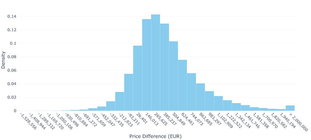
Figure 3: Distribution of Predicted Price Differences Between 2-Room (40m²) and 4-Room (90m²) Properties: This plot illustrates the distribution of predicted price differences, obtained via a Monte Carlo simulation, capturing the uncertainty in the model parameters. The mean price difference is approximately 405,697€, while the median is 337,281€, reflecting a slight right skew in the distribution. Key percentiles indicate a wide range of variability: the 10th percentile is -53,318€, the 25th percentile is 126,602€, the 75th percentile is 611,492€, and the 90th percentile is 956,934€. The standard deviation of 448,854€ highlights significant uncertainty in these predictions. Image by the author.
To understand what this means for Homer and Lisa’s situation, we need to estimate the distribution of price differences between the two properties. Using Monte Carlo simulation, we repeatedly draw samples from both predicted distributions and calculate their differences, building up the distribution shown in Figure 3. The results are sobering: while the mean difference suggests they would need to find an additional 405,697€, there is substantial uncertainty around this figure. In fact, approximately 13.4% of the simulated scenarios result in a negative price difference, meaning there is a non-negligible chance they could actually make money on the transaction. However, they should also be prepared for the possibility of needing significantly more money — there is a 25% chance they will need over 611,492€ — and 10% over 956,934€ — extra to make the upgrade.
This more complete picture of uncertainty gives Homer and Lisa a much better foundation for their decision-making than the seemingly precise single numbers provided by our earlier analyses.
Sometimes Less is More: The One With The Raw Data
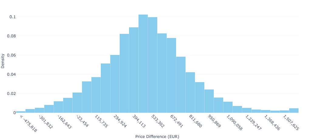
Figure 4: Distribution of Simulated Price Differences Between 2-Room (40m²) and 4-Room (90m²) Properties: This distribution is obtained through Monte Carlo simulation by randomly pairing actual transactions of 2-room (35–45m²) and 4-room (85–95m²) properties. The mean price difference is 484,672€ (median: 480,000€), with a substantial spread shown by the 90% percentile interval ranging from -52,810€ to 1,014,325€. The shaded region below zero, representing about 6.6% of scenarios, indicates cases where a 4-room property might be found at a lower price than a 2-room one. The distribution’s right skew suggests that while most price differences cluster around the median, there is a notable chance of encountering much larger differences, with 5% of cases exceeding 1,014,325€. Image by the author.
Rather than relying on sophisticated Bayesian modeling, we can gain clear insights from directly analyzing similar transactions. Looking at properties around Paris, we found 36,265 2-room flats (35–45m²) and 4,145 4-room properties (85–95m²), providing a rich dataset of actual market behavior.
The data shows substantial price variation. Two-room properties have a mean price of 329,080€ and a median price of 323,000€, with 90% of prices falling between 150,000€ and 523,650€. Four-room properties show even wider variation, with a mean price of 812,015€, a median price of 802,090€ and a 90% range from 315,200€ to 1,309,227€.
Using Monte Carlo simulation to randomly pair properties, we can estimate what Homer and Lisa might face. The mean price difference is 484,672€ and the median price difference is 480,000€, with the middle 50% of scenarios requiring between 287,488€ and 673,000€. Moreover, in 6.6% of cases, they might even find a 4-room property cheaper than their 2-room sale and make money.
This straightforward approach uses actual transactions rather than model predictions, making no assumptions about price relationships while capturing real market variability. For Homer and Lisa’s planning, the message is clear: while they should prepare for needing around 480,000€, they should be ready for scenarios requiring significantly more or less. Understanding this range of possibilities is crucial for their financial planning.
This simple technique works particularly well here because we have a dense dataset with over 40,000 relevant transactions across our target property categories. However, in many situations relying on predictive modeling, we might face sparse data. In such cases, we would need to interpolate between different data points or extrapolate beyond our available data. This is where Bayesian models are particularly powerful…
Final Remarks
The journey through these analytical approaches — OLS, log-normal modeling, Bayesian analysis, and Monte Carlo simulation — offers more than a range of price predictions. It highlights how we can handle uncertainty in predictive modeling with increasing sophistication. From the deceptively precise OLS estimate (439,795€) to the nuanced log-normal model (414,040€), and finally, to distributional insights provided by Bayesian and Monte Carlo methods (with means of 405,697€ and 484,672€, respectively), each method provides a unique perspective on the same problem.
This progression demonstrates when distributional thinking becomes beneficial. For high-stakes, one-off decisions like Homer and Lisa’s, understanding the full range of possibilities provides a clear advantage. In contrast, repetitive decisions with low individual stakes, like online ad placements, can often rely on simple point estimates. However, in domains where tail risks carry significant consequences — such as portfolio management or major financial planning — modeling the full distribution is not just beneficial but fundamentally wise.
It is important to acknowledge the real-world complexities simplified in this case study. Factors like interest rates, temporal dynamics, transaction costs, and other variables significantly influence real estate pricing. Our objective was not to develop a comprehensive housing price predictor but to illustrate, step-by-step, the progression from a naive single-point estimate to a full distribution.
It is worth noting that, given our primary aim of illustrating this progression — from point estimates to distributional thinking — we deliberately kept our models simple. The OLS and pseudo-GLM implementations were used without interaction terms — and thus without regularization or hyperparameter tuning — and minimal preprocessing was applied. While the high correlation between the number of rooms and surface area is not particularly problematic for predictive modeling in general, it can affect the sampling efficiency of the Markov chain Monte Carlo (MCMC) methods used in our Bayesian models by creating ridges in the posterior distribution that are harder to explore efficiently (indeed, we observed a strong ridge structure with correlation of -0.74 between these parameters, though effective sample sizes remained reasonable at about 50% of total samples, suggesting our inference should be sufficiently stable for our illustrative purposes). For the Bayesian approaches specifically, there is substantial room for improvement through defining more informative priors or the inclusion of additional covariates. While such optimizations might yield somewhat different numerical results, they would likely not fundamentally alter the key insights about the importance of considering full distributions rather than point estimates.
Finally, we must accept that even our understanding of uncertainty is uncertain. The confidence we place in distributional predictions depends on model assumptions and data quality. This “uncertainty about uncertainty” challenges us not only to refine our models but also to communicate their limitations transparently.
Embracing distributional thinking is not merely a technical upgrade — it is a mindset shift. Single-point predictions may feel actionable, but they often provide a false sense of precision, ignoring the inherent variability of outcomes. By considering the full spectrum of possibilities, we equip ourselves to make better-informed decisions and develop strategies that are better prepared for the randomness of the real world.
Sources
References
– Duan, N. (1983). Smearing estimate: A nonparametric retransformation method. Journal of the American Statistical Association, 78(383), 605–610. Available from https://www.jstor.org/stable/2288126. – Kahneman, D. (2011). Thinking, Fast and Slow. Kindle edition. ASIN B00555X8OA. – MacKenzie, D., & Spears, T. (2014). ‘The formula that killed Wall Street’: The Gaussian copula and modelling practices in investment banking. Social Studies of Science, 44(3), 393–417. Available from https://www.jstor.org/stable/43284238. – Patterson, S. (2023). Chaos Kings: How Wall Street Traders Make Billions in the New Age of Crisis. Kindle edition. ASIN B0BSB49L11. – Zuckerman, G. (2019). The Man Who Solved the Market: How Jim Simons Launched the Quant Revolution. Kindle edition. ASIN B07NLFC63Y.
Art and text by Loic Merckel. Licensed under CC BY 4.0. Originally published on 619.io. For discussions or engagement, feel free to refer to the LinkedIn version or Medium version. Otherwise, attribute the original source when sharing or reusing.
We use cookies on our website to give you the most relevant experience by remembering your preferences and repeat visits. By clicking “Accept”, you consent to the use of ALL the cookies.
This website uses cookies to improve your experience while you navigate through the website. Out of these, the cookies that are categorized as necessary are stored on your browser as they are essential for the working of basic functionalities of the website. We also use third-party cookies that help us analyze and understand how you use this website. These cookies will be stored in your browser only with your consent. You also have the option to opt-out of these cookies. But opting out of some of these cookies may affect your browsing experience.
Necessary cookies are absolutely essential for the website to function properly. These cookies ensure basic functionalities and security features of the website, anonymously.
Cookie
Duration
Description
cookielawinfo-checkbox-analytics
11 months
This cookie is set by GDPR Cookie Consent plugin. The cookie is used to store the user consent for the cookies in the category "Analytics".
cookielawinfo-checkbox-functional
11 months
The cookie is set by GDPR cookie consent to record the user consent for the cookies in the category "Functional".
cookielawinfo-checkbox-necessary
11 months
This cookie is set by GDPR Cookie Consent plugin. The cookies is used to store the user consent for the cookies in the category "Necessary".
cookielawinfo-checkbox-others
11 months
This cookie is set by GDPR Cookie Consent plugin. The cookie is used to store the user consent for the cookies in the category "Other.
cookielawinfo-checkbox-performance
11 months
This cookie is set by GDPR Cookie Consent plugin. The cookie is used to store the user consent for the cookies in the category "Performance".
viewed_cookie_policy
11 months
The cookie is set by the GDPR Cookie Consent plugin and is used to store whether or not user has consented to the use of cookies. It does not store any personal data.
Functional cookies help to perform certain functionalities like sharing the content of the website on social media platforms, collect feedbacks, and other third-party features.
Performance cookies are used to understand and analyze the key performance indexes of the website which helps in delivering a better user experience for the visitors.
Analytical cookies are used to understand how visitors interact with the website. These cookies help provide information on metrics the number of visitors, bounce rate, traffic source, etc.
Advertisement cookies are used to provide visitors with relevant ads and marketing campaigns. These cookies track visitors across websites and collect information to provide customized ads.