
avoid the outdated methods of integrating AI into your coding workflow by going beyond ChatGPT
Originally appeared here:
The Smarter Way of Using AI in Programming
Go Here to Read this Fast! The Smarter Way of Using AI in Programming

avoid the outdated methods of integrating AI into your coding workflow by going beyond ChatGPT
Originally appeared here:
The Smarter Way of Using AI in Programming
Go Here to Read this Fast! The Smarter Way of Using AI in Programming
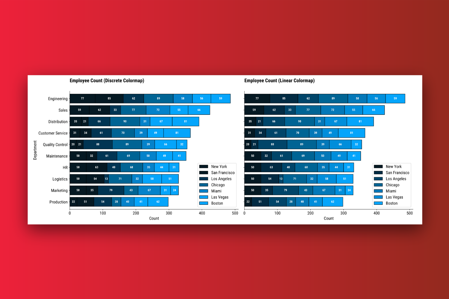

Actionable guide on how to bring custom colors to personalize your charts
Originally appeared here:
How to Create Custom Color Palettes in Matplotlib — Discrete vs. Linear Colormaps, Explained

Getting a handle on temperature, Top-k, Top-p, frequency, and presence penalties can be a bit of a challenge, especially when you’re just starting out with LLM hyperparameters. Terms like “Top-k” and “presence penalty” can feel a bit overwhelming at first.
When you look up “Top-k,” you might find a definition like: “Top-k sampling limits the model’s selection of the next word to only the top-k most probable options, based on their predicted probabilities.” That’s a lot to take in! But how does this actually help when you’re working on prompt engineering?
If you’re anything like me and learn best with visuals, let’s break these down together and make these concepts easy to understand once and for all.
Before we dive into LLM hyperparameters, let’s do a quick thought experiment. Imagine hearing the phrase “A cup of …”. Most of us would expect the next word to be something like “coffee” (or “tea” if you’re a tea person!) You probably wouldn’t think of “stars” or “courage” right away.
What’s happening here is that we’re instinctively predicting the most likely words to follow “A cup of …”, with “coffee” being a much higher likelihood than “stars”.
This is similar to how LLMs work — they calculate the probabilities of possible next words and choose one based on those probabilities.
So on a high level, the hyperparameters are ways to tune how we select the next probable words.
Let’s start with the most common hyperparameter:
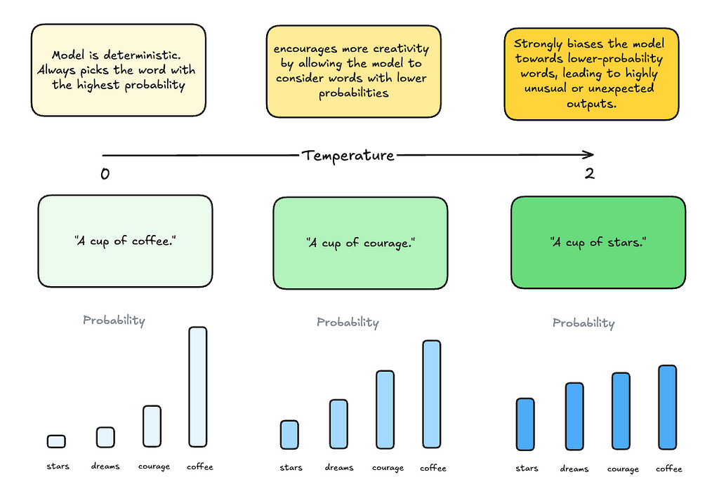
Temperature controls the randomness of the models’ output. A lower temperature makes the output more deterministic, favoring more likely words, while a higher temperature allows for more creativity by considering less likely words.
In our “A cup of…” example, setting the temperature to 0 makes the model favor the most likely word, which is “coffee”.
As temperature increases, the sampling probabilities between different words start to even out, prompting the model to generate highly unusal or unexpected outputs.
Note, that setting the temperature to 0 still doesn’t make the model completely deterministic, though it gets very close.
Use cases
Max tokens define the maximum number of tokens (which can be words or parts of words) the model can generate in its responses. Tokens are the smallest units of text that a model processes.
Relationship between tokens and words:
Use cases
Top-k sampling restricts the model from selecting from the top k most likely next words. By narrowing the choices, it helps reduce the chances of generating irrelevant or nonsensical outputs.
In the diagram below, if we set k to 2, the model will only consider the two most likely next words — in this case, ‘coffee’ and ‘courage.’ These two words are then resampled, with their probabilities adjusted to sum to 1, ensuring one of them is chosen.

Use cases:
Top-p sampling selects the smallest set of words whose combined probability exceeds a threshold p (e.g., 0.9), allowing for a more context-sensitive choice of words.
In the diagram below, we start with the most probable word, ‘coffee,’ which has a probability of 0.6. Since this is less than our threshold of p = 0.9, we add the next word, ‘courage,’ with a probability of 0.2. Together, these give us a total probability of 0.8, which is still below 0.9. Finally, we consider the word ‘dreams’ with a probability of 0.13, bringing the total to 0.93, which exceeds 0.9. At this point, we stop, having selected the first two most probable words.

Use cases:
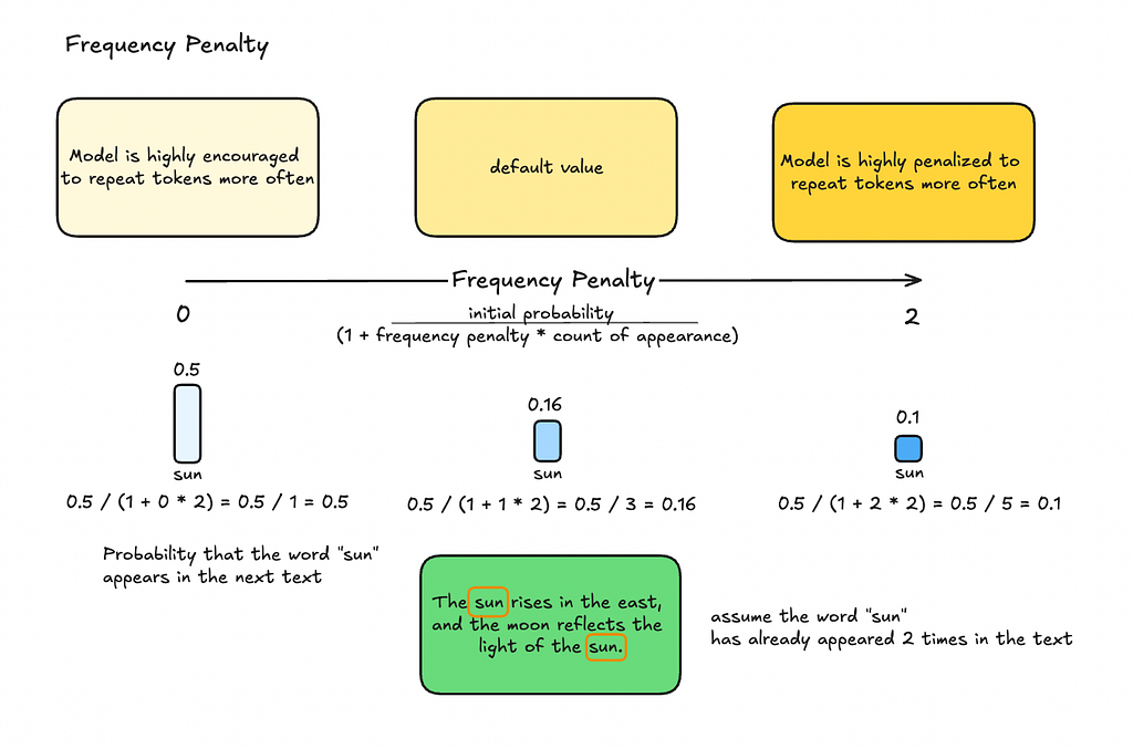
A frequency penalty reduces the likelihood of the model repeating the same word within the text, promoting diversity and minimizing redundancy in the output. By applying this penalty, the model is encouraged to introduce new words instead of reusing ones that have already appeared.
The frequency penalty is calculated using the formula:
Adjusted probability = initial probability / (1 + frequency penalty * count of appearance)
For example, let’s say that the word “sun” has a probability of 0.5, and it has already appeared twice in the text. If we set the frequency penalty to 1, the adjusted probability for “sun” would be:
Adjusted probability = 0.5 / (1 + 1 * 2) = 0.5 / 3 = 0.16
Use cases:
The presence penalty is similar to the frequency penalty but with one key difference: it penalizes the model for reusing any word or phrase that has already been mentioned, regardless of how often it appears.
In other words, repeating the word 2 times is as bad as repeating it 20 times.
The formula for adjusting the probability with a presence penalty is:
Adjusted probability = initial probability / (1 + presence penalty * presence)
Let’s revisit the earlier example with the word “sun”. Instead of multiplying the penalty by the frequency of how many times “sun” has appeared, we simply check whether it has appeared at all — in this case, it has, so we count it as 1.
If we set the presence penalty to 1, the adjusted probability would be:
Adjusted probability = 0.5 / (1 + 1 * 1) = 0.5 / 2 = 0.25
This reduction makes it less likely for the model to choose “sun” again, encouraging the use of new words or phrases, even if “sun” has only appeared once in the text.

Use cases:
Now that we’ve gone over the basics, let’s dive into how frequency and presence penalties are often used together. Just a heads-up, though — they’re powerful tools, but it’s important to use them with a bit of caution to get the best results.
When to use them:
When to not use them
By now, you should have a clearer picture of how temperature, Top-k, Top-p, frequency, and presence penalties work together to shape the output of your language model. And if it still feels a bit tricky, that’s totally okay — these concepts can take some time to fully click. Just keep experimenting and exploring, and you’ll get the hang of it before you know it.
If you find visual content like this helpful and want more, we’d love to see you in our Discord community. It’s a space where we share ideas, help each other out, and learn together.
A visual explanation of LLM hyperparameters was originally published in Towards Data Science on Medium, where people are continuing the conversation by highlighting and responding to this story.
Originally appeared here:
A visual explanation of LLM hyperparameters
Go Here to Read this Fast! A visual explanation of LLM hyperparameters


Originally appeared here:
Provide a personalized experience for news readers using Amazon Personalize and Amazon Titan Text Embeddings on Amazon Bedrock


Easy, user-friendly caching that tailors to all your needs
Originally appeared here:
Let’s Write a Composable, Easy-to-Use Caching Package in Python
Go Here to Read this Fast! Let’s Write a Composable, Easy-to-Use Caching Package in Python


How pruning, knowledge distillation, and 4-bit quantization can make advanced AI models more accessible and cost-effective
Originally appeared here:
Mistral-NeMo: 4.1x Smaller with Quantized Minitron
Go Here to Read this Fast! Mistral-NeMo: 4.1x Smaller with Quantized Minitron