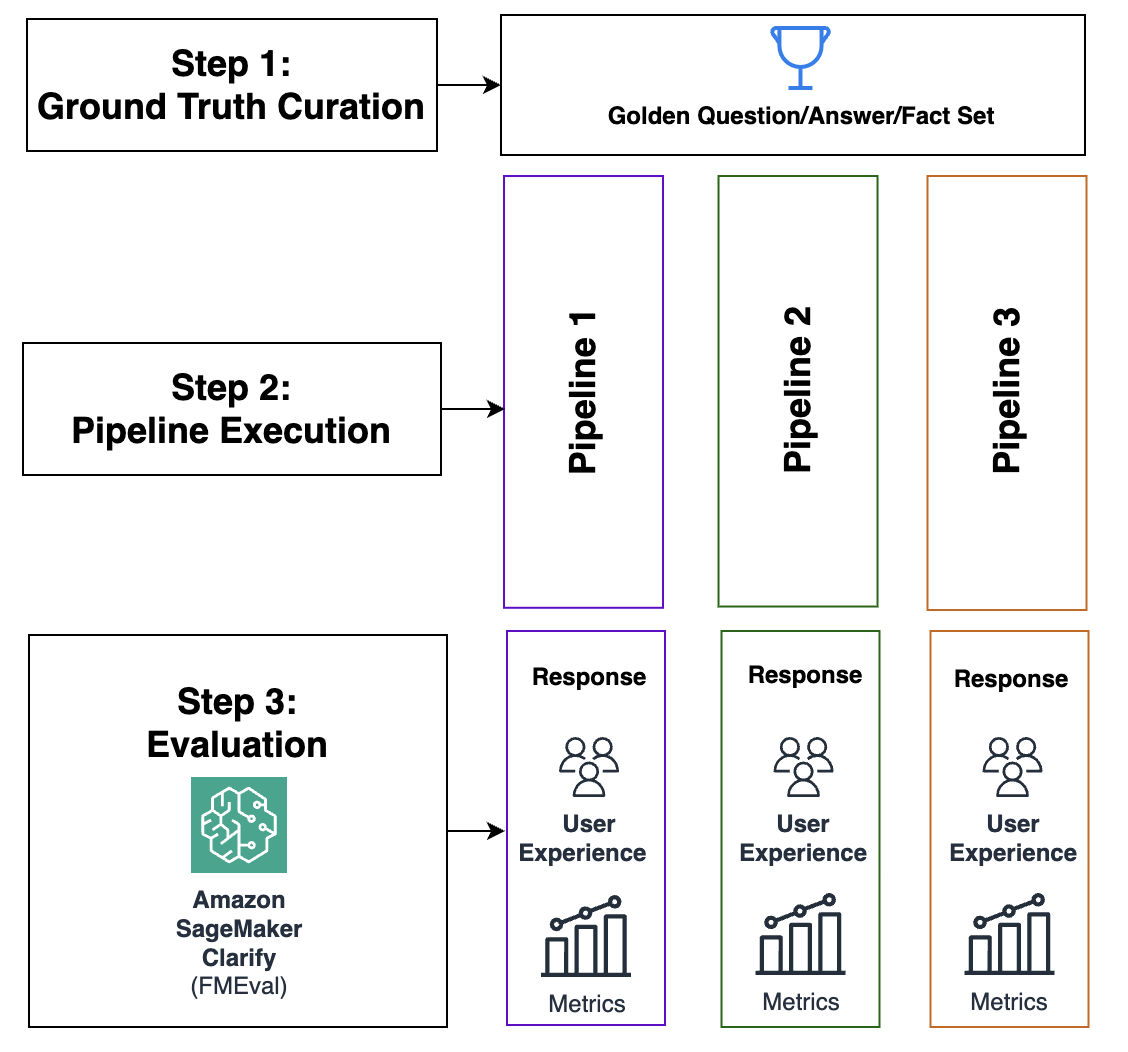
In this post, we discuss best practices for working with Foundation Model Evaluations Library (FMEval) in ground truth curation and metric interpretation for evaluating question answering applications for factual knowledge and quality.
Data science is at its best out in the real world. I intend to share insights from various productionized projects I have been involved in.
During my years working as a Data Scientist, I have met a lot of students interested in becoming one themselves, or newly graduated just starting out. Starting a career in data science, like any field, involves a steep learning curve.
One, very good, question that I keep getting is: I have learned a lot about the theoretical aspects of data science, but what does a real world example look like?
I want to share small pieces of work, from different projects I have been working on throughout my career. Even though some might be a few years old, I will only write about subjects which I still find relevant. I will try to keep the overarching picture clear and concise, so that new aspiring colleagues will get a grasp of what might be coming up. But I also want to stop and look into details, which I hope that more experienced developers might get some insights out of.
Business Case
Let’s now delve into the specific business case that drove this initiative. The team included a project manager, client stakeholders, and myself. The client needed a way to forecast the usage of a specific service. The reason behind this was resource allocation for maintaining the service and dynamic pricing. Experience with behaviour about the service usage was mostly kept within skilled coworkers, and this application was a way to be more resilient towards them retiring together with their knowledge. Also, the onboarding process of new hirings was thought to be easier with this kind of tool at hand.
Data and Analytical Setup
The data had a lot of features, both categorical and numerical. For the use case, there was a need to forecast the usage with a dynamical horizon, i.e. a need to make predictions for different periods of time into the future. There were also many, correlated and uncorrelated, values needed to be forecasted.
These multivariate time series made the attention mostly focused on experimenting with time series based models. But ultimately, Tabnet was adopted, a model that processes data as tabular.
There are several interesting features in the Tabnet architecture. This article will not delve into model details. But for the theoretical background I recommend doing some research. If you don’t find any good resources, I find this article a good overview or this paper for a more in depth exploration.
As a hyper parameter tuning framework, Optuna was used. There are also other frameworks in Python to use, but I have yet to find a reason not to use Optuna. Optuna was used as a Bayesian hyperparameter tuning, saved to disk. Other features utilized are early stopping and warm starting. Early stopping is used for resource saving purposes, not letting non promising looking trials run for too long. Warm starting is the ability to start from previous trials. This I find useful when new data arrives, and not having to start the tuning from scratch.
The initial parameter widths, will be set as recommended in the Tabnet documentation or from the parameter ranges discussed in the Tabnet paper.
To convey for the heteroscedastic nature of the residuals, Tabnet was implemented as a quantile regression model. To do this, or for implementing any model in this fashion, the pinball loss function, with suitable upper and lower quantiles, was used. This loss function has a skewed loss function, punishing errors unequally depending if they are positive or negative.
Walkthrough with Code
The requirements used for these snippets are as follows.
pytorch-tabnet==4.1.0
optuna==3.6.1
pandas==2.1.4
Code for defining the model.
import os
from pytorch_tabnet.tab_model import TabNetRegressor import pandas as pd import numpy as np
As a data manipulation framework, Pandas was used. I would also recommend using Polars, as a more efficient framework.
The Tabnet implementation comes with a pre-built local and global feature importance attribute to the fitted model. The inner workings on this can be studied in the article posted previous, but as the business use case goes this serves two purposes:
Sanity check — client can validate the model.
Business insights — the model can provide new insights about the business to the client.
together with the subject matter experts. In the end application, the interpretability was included to be displayed to the user. Due to data anonymization, there will not be a deep dive into interpretability in this article, but rather save it for a case where the true features going into the model can be discussed and displayed.
study = optuna.create_study(direction='minimize', storage='sqlite:///db.sqlite3', study_name=model_name, load_if_exists=True)
study.optimize(objective, n_trials=50)
The data are being split into a training, validation and testing set. The usage for the different datasets are:
Train. This is the dataset the model learns from. Consists in this project of 80%.
Validation. Is the dataset Optuna calculates its metrics from, and hence the metric optimized for. 10% of the data for this project.
Test. This is the dataset used to determine the true model performance. If this metric is not good enough, it might be worth going back to investigating other models. This dataset is also used to decide when it is time to stop the hyper parameter tuning. It is also on the basis of this dataset the KPI’s are derived and visualisations shared with the stakeholders.
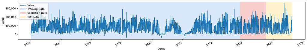
One final note is that to mimic the behavior of when the model is deployed, as much as possible, the datasets is being split on time. This means that the data from the first 80% of the period goes into the training part, the next 10% goes into validation and the most recent 10% into testing.
Illustration of time series data split. Plots created by the author.
For the example presented here, the trials are saved to disk. A more common approach is to save it to a cloud storage for better accessibility and easier maintenance. Optuna also comes with a UI for visualization, which can be spin up running the following command in the terminal.
pip install optuna-dashboard

cd /path/to/directory_with-db.sqlite3/

optuna-dashboard sqlite:///db.sqlite3
A manual task for sanity checking the parameter tuning, is to see how close to the sampling limits, the optimal parameters are. If they are reasonably far away from the bounds set, there is no need to look further into broadening the search space.
An in-depth look into what is displayed from the tuning can be found here.
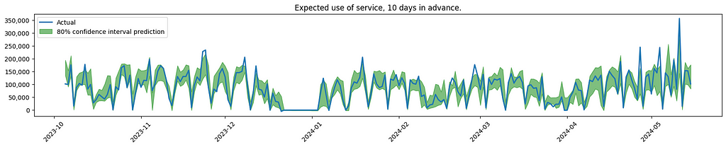
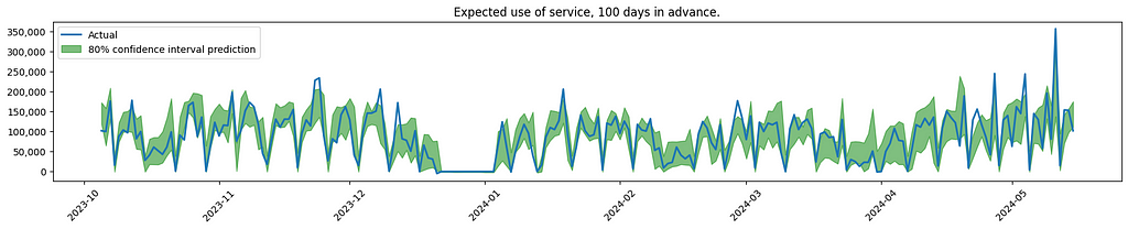
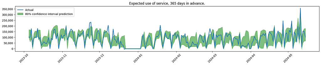
And here is a visualisation of some of the results.
Visualisation of model performance. Plots created by the author.
Conclusions and client remarks.
The graph indicates increased uncertainty when forecasting service usage further into the future. This is to be expected, also confirmed by the client.
As noticed, the model is having difficulties finding the spikes that are out of the ordinary. In the real use case, the effort was focused on looking into more sources of data, to see if the model could better predict these outliers.
In the final product there was also introduced a novelty score for the data point predicted, using the library Deepchecks. This came out of discussions with the client, trying to detect data drift and also for user insights into the data. In another article, there will be a deep dive on how this could be developed.
Thank you for reading!
I hope you found this article useful and/or inspiring. If you have any comments or question, please reach out! You can also connect with me on LinkedIn.
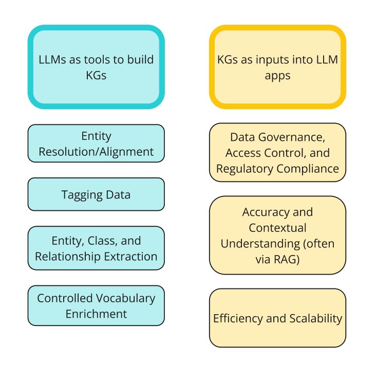
My last blog post was about how to implement knowledge graphs (KGs) and Large Language Models (LLMs) together at the enterprise level. In that post, I went through the two ways KGs and LLMs are interacting right now: LLMs as tools to build KGs; and KGs as inputs into LLM or GenAI applications. The diagram below shows the two sides of integrations and the different ways people are using them together.
Image by author
In this post, I will focus on one popular way KGs and LLMs are being used together: RAG using a knowledge graph, sometimes called Graph RAG, GraphRAG, GRAG, or Semantic RAG. Retrieval-Augmented Generation (RAG) is about retrieving relevant information to augment a prompt that is sent to an LLM, which generates a response. The idea is that, rather than sending your prompt directly to an LLM, which was not trained on your data, you can supplement your prompt with the relevant information needed for the LLM to answer your prompt accurately. The example I used in my previous post is copying a job description and my resume into ChatGPT to write a cover letter. The LLM is able to provide a much more relevant response to my prompt, ‘write me a cover letter,’ if I give it my resume and the description of the job I am applying for. Since knowledge graphs are built to store knowledge, they are a perfect way to store internal data and supplement LLM prompts with additional context, improving the accuracy and contextual understanding of the responses.
What is important, and I think often misunderstood, is that RAG and RAG using a KG (Graph RAG) are methodologies for combining technologies, not a product or technology themselves. No one invented, owns, or has a monopoly on Graph RAG. Most people can see the potential that these two technologies have when combined, however, and there are more and more studies proving the benefits of combining them.
Generally, there are three ways of using a KG for the retrieval part of RAG:
Vector-based retrieval: Vectorize your KG and store it in a vector database. If you then vectorize your natural language prompt, you can find vectors in the vector database that are most similar to your prompt. Since these vectors correspond to entities in your graph, you can return the most ‘relevant’ entities in the graph given a natural language prompt. Note that you can do vector-based retrieval without a graph. That is actually the original way RAG was implemented, sometimes called Baseline RAG. You’d vectorize your SQL database or content and retrieve it at query time.
Prompt-to-query retrieval: Use an LLM to write a SPARQL or Cypher query for you, use the query against your KG, and then use the returned results to augment your prompt.
Hybrid (vector + SPARQL): You can combine these two approaches in all kinds of interesting ways. In this tutorial, I will demonstrate some of the ways you can combine these methods. I will primarily focus on using vectorization for the initial retrieval and then SPARQL queries to refine the results.
There are, however, many ways of combining vector databases and KGs for search, similarity, and RAG. This is just an illustrative example to highlight the pros and cons of each individually and the benefits of using them together. The way I am using them together here — vectorization for initial retrieval and then SPARQL for filtering — is not unique. I have seen this implemented elsewhere. A good example I have heard anecdotally was from someone at a large furniture manufacturer. He said the vector database might recommend a lint brush to people buying couches, but the knowledge graph would understand materials, properties, and relationships and would ensure that the lint brush is not recommended to people buying leather couches.
In this tutorial I will:
Vectorize a dataset into a vector database to test semantic search, similarity search, and RAG (vector-based retrieval)
Turn the data into a KG to test semantic search, similarity search, and RAG (prompt-to-query retrieval, though really more like query retrieval since I’m just using SPARQL directly rather than having an LLM turn my natural language prompt into a SPARQL query)
Vectorize dataset with tags and URIs from the knowledge graph into a vector database (what I’ll refer to as a “vectorized knowledge graph”) and test semantic search, similarity, and RAG (hybrid)
The goal is to illustrate the differences between KGs and vector databases for these capabilities and to show some of the ways they can work together. Below is a high-level overview of how, together, vector databases and knowledge graphs can execute advanced queries.
Image by author
If you don’t feel like reading any further, here is the TL;DR:
Vector databases can run semantic searches, similarity calculations and some basic forms of RAG pretty well with a few caveats. The first caveat is that the data I am using contains abstracts of journal articles, i.e. it has a good amount of unstructured text associated with it. Vectorization models are trained primarily on unstructured data and so perform well when given chunks of text associated with entities.
That being said, there is very little overhead in getting your data into a vector database and ready to be queried. If you have a dataset with some unstructured data in it, you can vectorize and start searching in 15 minutes.
Not surprisingly, one of the biggest drawbacks of using a vector database alone is the lack of explainability. The response might have three good results and one that doesn’t make much sense, and there is no way to know why that fourth result is there.
The chance of unrelated content being returned by a vector database is a nuisance for search and similarity, but a huge problem for RAG. If you’re augmenting your prompt with four articles and one of them is about a completely unrelated topic, the response from the LLM is going to be misleading. This is often referred to as ‘context poisoning’.
What is especially dangerous about context poisoning is that the response isn’t necessarily factually inaccurate, and it isn’t based on an inaccurate piece of data, it’s just using the wrong data to answer your question. The example I found in this tutorial is for the prompt, “therapies for mouth neoplasms.” One of the retrieved articles was about a study conducted on therapies for rectal cancer, which was sent to the LLM for summarization. I’m no doctor but I’m pretty sure the rectum’s not part of the mouth. The LLM accurately summarized the study and the effects of different therapy options on both mouth and rectal cancer, but didn’t always mention type of cancer. The user would therefore be unknowingly reading an LLM describe different treatment options for rectal cancer, after having asked the LLM to describe treatments for mouth cancer.
The degree to which KGs can do semantic search and similarity search well is a function of the quality of your metadata and the controlled vocabularies the metadata connects to. In the example dataset in this tutorial, the journal articles have all been tagged already with topical terms. These terms are part of a rich controlled vocabulary, the Medical Subject Headings (MeSH) from the National Institutes of Health. Because of that, we can do semantic search and similarity relatively easily out of the box.
There is likely some benefit of vectorizing a KG directly into a vector database to use as your knowledge base for RAG, but I didn’t do that for this tutorial. I just vectorized the data in tabular format but added a column for a URI for each article so I could connect the vectors back to the KG.
One of the biggest strengths of using a KG for semantic search, similarity, and RAG is in explainability. You can always explain why certain results were returned: they were tagged with certain concepts or had certain metadata properties.
Another benefit of the KG that I did not foresee is something sometimes called, “enhanced data enrichment” or “graph as an expert” — you can use the KG to expand or refine your search terms. For example, you can find similar terms, narrower terms, or terms related to your search term in specific ways, to expand or refine your query. For example, I might start with searching for “mouth cancer,” but based on my KG terms and relationships, refine my search to “gingival neoplasms and palatal neoplasms.”
One of the biggest obstacles to getting started with using a KG is that you need to build a KG. That being said, there are many ways to use LLMs to speed up the construction of a KG (figure 1 above).
One downside of using a KG alone is that you’ll need to write SPARQL queries to do everything. Hence the popularity of prompt-to-query retrieval described above.
The results from using Jaccard similarity on terms to find similar articles in the knowledge graph were poor. Without specification, the KG returned articles that had overlapping tags such as, “Aged”, “Male”, and “Humans”, that are probably not nearly as relevant as “Treatment Options” or “Mouth Neoplasms”.
Another issue I faced was that Jaccard similarity took forever (like 30 minutes) to run. I don’t know if there is a better way to do this (open to suggestions) but I am guessing that it is just very computationally intensive to find overlapping tags between an article and 9,999 other articles.
Since the example prompts I used in this tutorial were something simple like ‘summarize these articles’ — the accuracy of the response from the LLM (for both the vector-based and KG-based retrieval methods) was much more dependent on the retrieval than the generation. What I mean is that as long as you give the LLM the relevant context, it is very unlikely that the LLM is going to mess up a simple prompt like ‘summarize’. This would be very different if our prompts were more complicated questions of course.
Using the vector database for the initial search and then the KG for filtering provided the best results. This is somewhat obvious —you wouldn’t filter to get worse results. But that’s the point: it’s not that the KG necessarily improves results by itself, it’s that the KG provides you the ability to control the output to optimize your results.
Filtering results using the KG can improve the accuracy and relevancy based on the prompt, but it can also be used to customize results based on the person writing the prompt. For example, we may want to use similarity search to find similar articles to recommend to a user, but we’d only want to recommend articles that that person has access to. The KG allows for query-time access control.
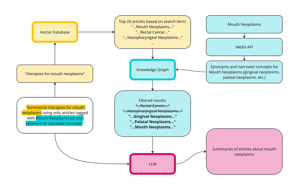
KGs can also help reduce the likelihood of context poisoning. In the RAG example above, we can search for ‘therapies for mouth neoplasms,’ in the vector database, but then filter for only articles that are tagged with mouth neoplasms (or related concepts).
I only focused on a simple implementation in this tutorial where we sent the prompt directly to the vector database and then filter the results using the graph. There are far better ways of doing this. For example, you could extract entities from the prompt that align with your controlled vocabulary and enrich them (with synonyms and narrower terms) using the graph; you could parse the prompt into semantic chunks and send them separately to the vector database; you could turn the RDF data into text before vectorizing so the language model understands it better, etc. Those are topics for future blog posts.
Step 1: Vector-based retrieval
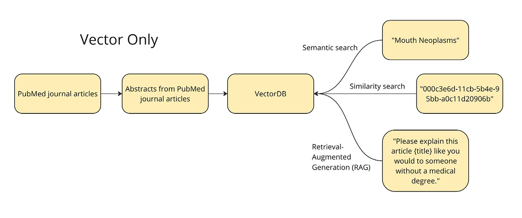
The diagram below shows the plan at a high level. We want to vectorize the abstracts and titles from journal articles into a vector database to run different queries: semantic search, similarity search, and a simple version of RAG. For semantic search, we will test a term like ‘mouth neoplasms’ — the vector database should return articles relevant to this topic. For similarity search, we will use the ID of a given article to find its nearest neighbors in the vector space i.e. the articles most similar to this article. Finally, vector databases allow for a form of RAG where we can supplement a prompt like, “please explain this like you would to someone without a medical degree,” with an article.
Image by author
I’ve decided to use this dataset of 50,000 research articles from the PubMed repository (License CC0: Public Domain). This dataset contains the title of the articles, their abstracts, as well as a field for metadata tags. These tags are from the Medical Subject Headings (MeSH) controlled vocabulary thesaurus. For the purposes of this part of the tutorial, we are only going to use the abstracts and the titles. This is because we are trying to compare a vector database with a knowledge graph and the strength of the vector database is in its ability to ‘understand’ unstructured data without rich metadata. I only used the top 10,000 rows of the data, just to make the calculations run faster.
Here is Weaviate’s official quickstart tutorial. I also found this article helpful in getting started.
from weaviate.util import generate_uuid5
import weaviate
import json
import pandas as pd

#Read in the pubmed data
df = pd.read_csv("PubMed Multi Label Text Classification Dataset Processed.csv")
Then we can establish a connection to our Weaviate cluster:
client = weaviate.Client(
    url = "XXX",  # Replace with your Weaviate endpoint
    auth_client_secret=weaviate.auth.AuthApiKey(api_key="XXX"),  # Replace with your Weaviate instance API key
    additional_headers = {
        "X-OpenAI-Api-Key": "XXX"  # Replace with your inference API key
    }
)
Before we vectorize the data into the vector database, we must define the schema. Here is where we define which columns from the csv we want to vectorize. As mentioned, for the purposes of this tutorial, to start, I only want to vectorize the title and abstract columns.
class_obj = { # Class definition "class": "articles",
For some reason, only 9997 of my rows were vectorized. ¯_(ツ)_/¯
Semantic search using vector database
When we talk about semantics in the vector database, we mean that the terms are vectorized into the vector space using the LLM API which has been trained on lots of unstructured content. This means that the vector takes the context of the terms into consideration. For example, if the term Mark Twain is mentioned many times near the term Samuel Clemens in the training data, the vectors for these two terms should be close to each other in the vector space. Likewise, if the term Mouth Cancer appears together with Mouth Neoplasms many times in the training data, we would expect the vector for an article about Mouth Cancer to be near an article about Mouth Neoplasms in the vector space.
You can check that it worked by running a simple query:
Article 1:“Gingival metastasis as first sign of multiorgan dissemination of epithelioid malignant mesothelioma.” This article is about a study conducted on people who had malignant mesothelioma (a form of lung cancer) that spread to their gums. The study was to test the effects of different treatments (chemotherapy, decortication, and radiotherapy) on the cancer. This seems like an appropriate article to return — it is about gingival neoplasms, a subset of mouth neoplasms.
Article 2:“Myoepithelioma of minor salivary gland origin. Light and electron microscopical study.” This article is about a tumor that was removed from a 14-year-old boy’s gum, had spread to part of the upper jaw, and was composed of cells which originated in the salivary gland. This also seems like an appropriate article to return — it is about a neoplasm that was removed from a boy’s mouth.
Article 3:“Metastatic neuroblastoma in the mandible. Report of a case.” This article is a case study of a 5-year-old boy who had cancer in his lower jaw. This is about cancer, but technically not mouth cancer — mandibular neoplasms (neoplasms in the lower jaw) are not a subset of mouth neoplasms.
This is what we mean by semantic search — none of these articles have the word ‘mouth’ anywhere in their titles or abstracts. The first article is about gingival (gums) neoplasms, a subset of mouth neoplasms. The second article is about a gingival neoplasms that originated in the subject’s salivary gland, both subsets of mouth neoplasms. The third article is about mandibular neoplasms — which is, technically, according to the MeSH vocabulary not a subset of mouth neoplasms. Still, the vector database knew that a mandible is close to a mouth.
Similarity search using vector database
We can also use the vector database to find similar articles. I chose an article that was returned using the mouth neoplasms query above titled, “Gingival metastasis as first sign of multiorgan dissemination of epithelioid malignant mesothelioma.” Using the ID for that article, I can query the vector database for all similar entities:
response = (
    client.query
    .get("articles", ["title", "abstractText"])
    .with_near_object({
        "id": "a7690f03-66b9-5d17-b765-8c6eb21f99c8" #id for a given article
    })
    .with_limit(10)
    .with_additional(["distance"])
    .do()
)

print(json.dumps(response, indent=2))
The results are ranked in order of similarity. Similarity is calculated as distance in the vector space. As you can see, the top result is the Gingival article — this article is the most similar article to itself.
The other articles are:
Article 4: “Feasability study of screening for malignant lesions in the oral cavity targeting tobacco users.” This is about mouth cancer, but about how to get tobacco smokers to sign up for screenings rather than on the ways they were treated.
Article 5: “Extended Pleurectomy and Decortication for Malignant Pleural Mesothelioma Is an Effective and Safe Cytoreductive Surgery in the Elderly.” This article is about a study on treating pleural mesothelioma (cancer in the lungs) with pleurectomy and decortication (surgery to remove cancer from the lungs) in the elderly. So this is similar in that it is about treatments for mesothelioma, but not about gingival neoplasms.
Article 3 (from above): “Metastatic neuroblastoma in the mandible. Report of a case.” Again, this is the article about the 5-year-old boy who had cancer in his lower jaw. This is about cancer, but technically not mouth cancer, and this is not really about treatment outcomes like the gingival article.
All of these articles, one could argue, are similar to our original gingival article. It is difficult to assess how similar they are and to therefore assess how well the similarity search performed because that is largely a matter of what the user means by similar. Were you interested in other articles about treatments for mesothelioma and the fact that the first article is about how it spread to the gums is irrelevant? In that case, Article 5 is the most similar. Or are you interested in reducing any type of mouth cancer, whether through treatment or prevention? In that case, Article 4 is the most similar. One drawback of the vector database, is that it is a black box — we have no idea why these articles were returned.
Retrieval-Augmented Generation (RAG) using a vector database
Here is how you can use the vector database to retrieve results which are then sent to an LLM for summarization — an example of RAG.
response = (
    client.query
    .get("articles", ["title", "abstractText"])
    .with_near_text({"concepts": ["Gingival metastasis as first sign of multiorgan dissemination of epithelioid malignant mesothelioma"]})
    .with_generate(single_prompt="Please explain this article {title} like you would to someone without a medical degree.")
    .with_limit(1)
    .do()
)

print(json.dumps(response, indent=4))
You can see the response below:
“Sure! This article is talking about a case where a person had a type of cancer called epithelioid malignant mesothelioma. This cancer usually starts in the lining of the lungs or abdomen. However, in this case, the first sign of the cancer spreading to other parts of the body was seen in the gums (gingiva). This is called gingival metastasis.nnMetastasis means that cancer cells have spread from the original tumor to other parts of the body. In this case, the cancer had spread to the gums before spreading to other organs. This is important because it shows that the cancer was already advanced and had spread to multiple organs before it was even detected.nnOverall, this article highlights the importance of early detection and monitoring of cancer, as well as the potential for cancer to spread to unexpected parts of the body.”
I am actually disappointed by this response. The abstract clearly explains that this is a study that follows 13 patients with metastatic malignant mesothelioma that underwent different treatments and the outcomes. The RAG output describes the article as about ‘a person’ and doesn’t mention the study at all.
Rather than just summarize one article, let’s try to summarize several. In this next example, we use the same search term as above (Mouth Neoplasms) and then send the top three articles along with a prompt, ‘Summarize the key information here in bullet points. Make it understandable to someone without a medical degree,’ to an LLM.
response = ( client.query .get(collection_name, ["title", "abstractText"]) .with_near_text({"concepts": ["Mouth Neoplasms"]}) .with_limit(3) .with_generate(grouped_task="Summarize the key information here in bullet points. Make it understandable to someone without a medical degree.") .do() )
- Metastatic malignant mesothelioma to the oral cavity is rare, with more cases in jaw bones than soft tissue
- Average survival rate for this type of cancer is 9-12 months
- Study of 13 patients who underwent neoadjuvant chemotherapy and surgery showed a median survival of 11 months
- One patient had a gingival mass as the first sign of multiorgan recurrence of mesothelioma
- Biopsy of new growing lesions, even in uncommon sites, is important for patients with a history of mesothelioma
- Myoepithelioma of minor salivary gland origin can show features indicative of malignant potential
- Metastatic neuroblastoma in the mandible is very rare and can present with osteolytic jaw defects and looseness of deciduous molars in children
This looks better to me than the previous response — it mentions the study conducted in Article 1, the treatments, and the outcomes. The second to last bullet is about the “Myoepithelioma of minor salivary gland origin. Light and electron microscopical study,” article and seems to be an accurate one line description. The final bullet is about Article 3 referenced above, and, again, seems to be an accurate one line description.
Step 2: use a knowledge graph for data retrieval
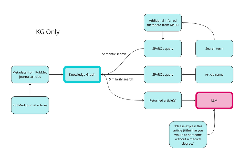
Here is a high-level overview of how we use a knowledge graph for semantic search, similarity search, and RAG:
Image by author
The first step of using a knowledge graph to retrieve your data is to turn your data into RDF format. The code below creates classes and properties for all of the data types, and then populates it with instances of articles and MeSH terms. I have also created properties for date published and access level and populated them with random values just as a demonstration.
from rdflib import Graph, RDF, RDFS, Namespace, URIRef, Literal from rdflib.namespace import SKOS, XSD import pandas as pd import urllib.parse import random from datetime import datetime, timedelta
# Create a new RDF graph g = Graph()
# Define namespaces schema = Namespace('http://schema.org/') ex = Namespace('http://example.org/') prefixes = { 'schema': schema, 'ex': ex, 'skos': SKOS, 'xsd': XSD } for p, ns in prefixes.items(): g.bind(p, ns)
# Function to clean and parse MeSH terms def parse_mesh_terms(mesh_list): if pd.isna(mesh_list): return [] return [term.strip().replace(' ', '_') for term in mesh_list.strip("[]'").split(',')]
# Function to create a valid URI def create_valid_uri(base_uri, text): if pd.isna(text): return None sanitized_text = urllib.parse.quote(text.strip().replace(' ', '_').replace('"', '').replace('<', '').replace('>', '').replace("'", "_")) return URIRef(f"{base_uri}/{sanitized_text}")
# Function to generate a random date within the last 5 years def generate_random_date(): start_date = datetime.now() - timedelta(days=5*365) random_days = random.randint(0, 5*365) return start_date + timedelta(days=random_days)
# Function to generate a random access value between 1 and 10 def generate_random_access(): return random.randint(1, 10)
# Load your DataFrame here # df = pd.read_csv('your_data.csv')
# Loop through each row in the DataFrame and create RDF triples for index, row in df.iterrows(): article_uri = create_valid_uri("http://example.org/article", row['Title']) if article_uri is None: continue
# Add random datePublished and access random_date = generate_random_date() random_access = generate_random_access() g.add((article_uri, date_published, Literal(random_date.date(), datatype=XSD.date))) g.add((article_uri, access, Literal(random_access, datatype=XSD.integer)))
# Add MeSH Terms mesh_terms = parse_mesh_terms(row['meshMajor']) for term in mesh_terms: term_uri = create_valid_uri("http://example.org/mesh", term) if term_uri is None: continue
# Link Article to MeSH Term g.add((article_uri, schema.about, term_uri))
# Serialize the graph to a file (optional) g.serialize(destination='ontology.ttl', format='turtle')
Semantic search using a knowledge graph
Now we can test semantic search. The word semantic is slightly different in the context of knowledge graphs, however. In the knowledge graph, we are relying on the tags associated with the documents and their relationships in the MeSH taxonomy for the semantics. For example, an article might be about Salivary Neoplasms (cancer in the salivary glands) but still be tagged with the term Mouth Neoplasms.
Rather than query all articles tagged with Mouth Neoplasms, we will also look for any concept narrower than Mouth Neoplasms. The MeSH vocabulary contains definitions of terms but it also contains relationships like broader and narrower.
triples = set() # Using a set to avoid duplicate entries for result in results["results"]["bindings"]: obj_label = result.get("oLabel", {}).get("value", "No label") triples.add(obj_label)
# Add the term itself to the list triples.add(term)
return list(triples) # Convert back to a list for easier handling
concepts = set() # Using a set to avoid duplicate entries for result in results["results"]["bindings"]: subject_label = result.get("narrowerConceptLabel", {}).get("value", "No label") concepts.add(subject_label)
return list(concepts) # Convert back to a list for easier handling
def get_all_narrower_concepts(term, depth=2, current_depth=1): # Create a dictionary to store the terms and their narrower concepts all_concepts = {}
# Initial fetch for the primary term narrower_concepts = get_narrower_concepts_for_term(term) all_concepts[term] = narrower_concepts
# If the current depth is less than the desired depth, fetch narrower concepts recursively if current_depth < depth: for concept in narrower_concepts: # Recursive call to fetch narrower concepts for the current concept child_concepts = get_all_narrower_concepts(concept, depth, current_depth + 1) all_concepts.update(child_concepts)
return all_concepts
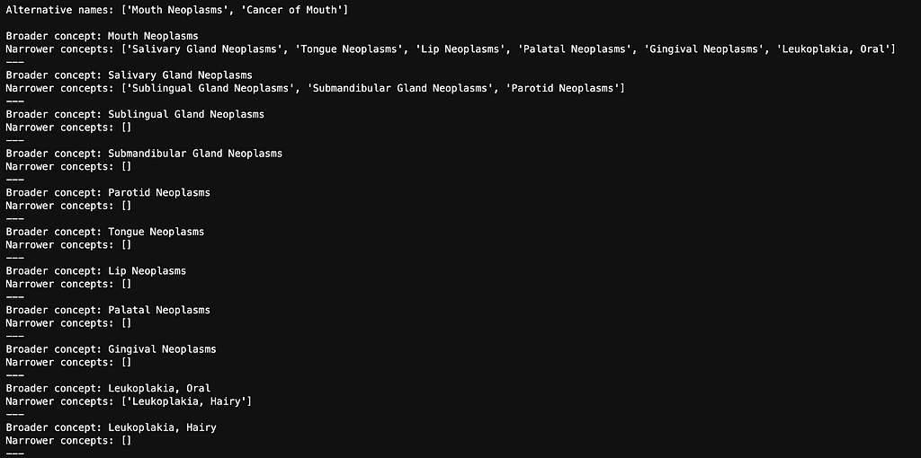
# Fetch alternative names and narrower concepts term = "Mouth Neoplasms" alternative_names = get_concept_triples_for_term(term) all_concepts = get_all_narrower_concepts(term, depth=2) # Adjust depth as needed
# Output alternative names print("Alternative names:", alternative_names) print()
# Output narrower concepts for broader, narrower in all_concepts.items(): print(f"Broader concept: {broader}") print(f"Narrower concepts: {narrower}") print("---")
Below are all of the alternative names and narrower concepts for Mouth Neoplasms.
def recurse_terms(term_dict): for term, narrower_terms in term_dict.items(): flat_list.append(term) if narrower_terms: recurse_terms(dict.fromkeys(narrower_terms, [])) # Use an empty dict to recurse
recurse_terms(concepts_dict) return flat_list
# Flatten the concepts dictionary flat_list = flatten_concepts(all_concepts)
Then we turn the terms into MeSH URIs so we can incorporate them into our SPARQL query:
#Convert the MeSH terms to URI
def convert_to_mesh_uri(term):
    formatted_term = term.replace(" ", "_").replace(",", "_").replace("-", "_")
    return URIRef(f"http://example.org/mesh/_{formatted_term}_")


# Convert terms to URIs
mesh_terms = [convert_to_mesh_uri(term) for term in flat_list]
Then we write a SPARQL query to find all articles that are tagged with ‘Mouth Neoplasms’, its alternative name, ‘Cancer of Mouth,’ or any of the narrower terms:
# Dictionary to store articles and their associated MeSH terms article_data = {}
# Run the query for each MeSH term for mesh_term in mesh_terms: results = g.query(query, initBindings={'meshTerm': mesh_term})
# Process results for row in results: article_uri = row['article']
if article_uri not in article_data: article_data[article_uri] = { 'title': row['title'], 'abstract': row['abstract'], 'datePublished': row['datePublished'], 'access': row['access'], 'meshTerms': set() }
# Add the MeSH term to the set for this article article_data[article_uri]['meshTerms'].add(str(row['meshTerm']))
# Rank articles by the number of matching MeSH terms ranked_articles = sorted( article_data.items(), key=lambda item: len(item[1]['meshTerms']), reverse=True )
# Get the top 3 articles top_3_articles = ranked_articles[:3]
# Output results for article_uri, data in top_3_articles: print(f"Title: {data['title']}") print("MeSH Terms:") for mesh_term in data['meshTerms']: print(f" - {mesh_term}") print()
The articles returned are:
Article 2 (from above):“Myoepithelioma of minor salivary gland origin. Light and electron microscopical study.”
Article 4 (from above): “Feasability study of screening for malignant lesions in the oral cavity targeting tobacco users.”
Article 6:“Association between expression of embryonic lethal abnormal vision-like protein HuR and cyclooxygenase-2 in oral squamous cell carcinoma.” This article is about a study to determine whether the presence of a protein called HuR is linked to a higher level of cyclooxygenase-2, which plays a role in cancer development and the spread of cancer cells. Specifically, the study was focused on oral squamous cell carcinoma, a type of mouth cancer.
These results are not dissimilar to what we got from the vector database. Each of these articles is about mouth neoplasms. What is nice about the knowledge graph approach is that we do get explainability — we know exactly why these articles were chosen. Article 2 is tagged with “Gingival Neoplasms”, and “Salivary Gland Neoplasms.” Articles 4 and 6 are both tagged with “Mouth Neoplasms.” Since Article 2 is tagged with 2 matching terms from our search terms, it is ranked highest.
Similarity search using a knowledge graph
Rather than using a vector space to find similar articles, we can rely on the tags associated with articles. There are different ways of doing similarity using tags, but for this example, I will use a common method: Jaccard Similarity. We will use the gingival article again for comparison across methods.
from rdflib import Graph, URIRef from rdflib.namespace import RDF, RDFS, Namespace, SKOS import urllib.parse
# Function to calculate Jaccard similarity and return overlapping terms def jaccard_similarity(set1, set2): intersection = set1.intersection(set2) union = set1.union(set2) similarity = len(intersection) / len(union) if len(union) != 0 else 0 return similarity, intersection
# Load the RDF graph g = Graph() g.parse('ontology.ttl', format='turtle')
def get_article_uri(title): # Convert the title to a URI-safe string safe_title = urllib.parse.quote(title.replace(" ", "_")) return URIRef(f"http://example.org/article/{safe_title}")
# Query all articles and their MeSH terms query = """ PREFIX schema: <http://schema.org/> PREFIX ex: <http://example.org/> PREFIX rdfs: <http://www.w3.org/2000/01/rdf-schema#>
SELECT ?article ?meshTerm WHERE { ?article a ex:Article ; schema:about ?meshTerm . ?meshTerm a ex:MeSHTerm . } """ results = g.query(query)
mesh_terms_other_articles = {} for row in results: article = str(row['article']) mesh_term = str(row['meshTerm']) if article not in mesh_terms_other_articles: mesh_terms_other_articles[article] = set() mesh_terms_other_articles[article].add(mesh_term)
# Calculate Jaccard similarity similarities = {} overlapping_terms = {} for article, mesh_terms in mesh_terms_other_articles.items(): if article != str(article_uri): similarity, overlap = jaccard_similarity(mesh_terms_given_article, mesh_terms) similarities[article] = similarity overlapping_terms[article] = overlap
# Sort by similarity and get top 5 top_similar_articles = sorted(similarities.items(), key=lambda x: x[1], reverse=True)[:15]
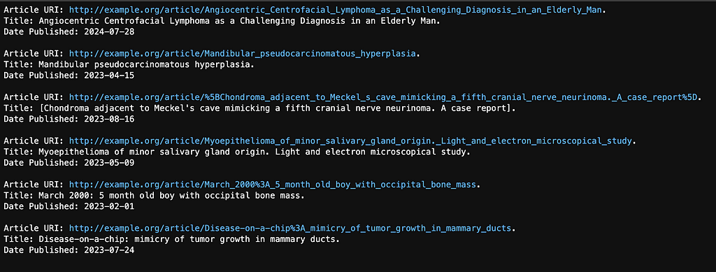
# Print results print(f"Top 15 articles similar to '{title}':") for article, similarity in top_similar_articles: print(f"Article URI: {article}") print(f"Jaccard Similarity: {similarity:.4f}") print(f"Overlapping MeSH Terms: {overlapping_terms[article]}") print()
# Example usage article_title = "Gingival metastasis as first sign of multiorgan dissemination of epithelioid malignant mesothelioma." find_similar_articles(article_title)
The results are below. Since we are searching on the Gingival article again, that is the most similar article, which is what we would expect. The other results are:
Article 7:“Calcific tendinitis of the vastus lateralis muscle. A report of three cases.” This article is about calcific tendinitis (calcium deposits forming in tendons) in the vastus lateralis muscle (a muscle in the thigh). This has nothing to do with mouth neoplasms.
Article 8:“What is the optimal duration of androgen deprivation therapy in prostate cancer patients presenting with prostate specific antigen levels.” This article is about how long prostate cancer patients should receive a specific treatment (androgen deprivataion therapy). This is about a treatment for cancer (radiotherapy), but not mouth cancer.
Article 9:CT scan cerebral hemisphere asymmetries: predictors of recovery from aphasia. This article is about how differences between the left and right sides of the brain (cerebral hemisphere assymetries) might predict how well someone recovers from aphasia after a stroke.
The best part of this method is that, because of the way we are calculating similarity here, we can see WHY the other articles are similar — we see exactly which terms are overlapping i.e. which terms are common on the Gingival article and each of the comparisons.
The downside of explainability is that we can see that these do not seem like the most similar articles, given the previous results. They all have three terms in common (Aged, Male, and Humans) that are probably not nearly as relevant as Treatment Options or Mouth Neoplasms. You could re-calculate using some weight based on the prevalence of the term across the corpus — Term Frequency-Inverse Document Frequency (TF-IDF) — which would probably improve the results. You could also select the tagged terms that are most relevant for you when conducting similarity for more control over the results.
The biggest downside of using Jaccard similarity on terms in a knowledge graph for calculating similarity is the computational efforts — it took like 30 minutes to run this one calculation.
RAG using a knowledge graph
We can also do RAG using just the knowledge graph for the retrieval part. We already have a list of articles about mouth neoplasms saved as results from the semantic search above. To implement RAG, we just want to send these articles to an LLM and ask it to summarize the results.
First we combine the titles and abstracts for each of the articles into one big chunk of text called combined_text:
# Function to combine titles and abstracts
def combine_abstracts(top_3_articles):
    combined_text = "".join(
        [f"Title: {data['title']} Abstract: {data['abstract']}" for article_uri, data in top_3_articles]
    )
    return combined_text

# Combine abstracts from the top 3 articles
combined_text = combine_abstracts(top_3_articles)
print(combined_text)
We then set up a client so that we can send this text directly to an LLM:
import openai

# Set up your OpenAI API key
api_key = "YOUR API KEY"
openai.api_key = api_key
Then we give the context and the prompt to the LLM:
def generate_summary(combined_text):
    response = openai.Completion.create(
        model="gpt-3.5-turbo-instruct",
        prompt=f"Summarize the key information here in bullet points. Make it understandable to someone without a medical degree:nn{combined_text}",
        max_tokens=1000,
        temperature=0.3
    )

    # Get the raw text output
    raw_summary = response.choices[0].text.strip()

    # Split the text into lines and clean up whitespace
    lines = raw_summary.split('n')
    lines = [line.strip() for line in lines if line.strip()]

    # Join the lines back together with actual line breaks
    formatted_summary = 'n'.join(lines)

    return formatted_summary

# Generate and print the summary
summary = generate_summary(combined_text)
print(summary)
The results look as follows:
- A 14-year-old boy had a gingival tumor in his anterior maxilla that was removed and studied by light and electron microscopy
- The tumor was made up of myoepithelial cells and appeared to be malignant
- Electron microscopy showed that the tumor originated from a salivary gland
- This is the only confirmed case of a myoepithelioma with features of malignancy
- A feasibility study was conducted to improve early detection of oral cancer and premalignant lesions in a high incidence region
- Tobacco vendors were involved in distributing flyers to invite smokers for free examinations by general practitioners
- 93 patients were included in the study and 27% were referred to a specialist
- 63.6% of those referred actually saw a specialist and 15.3% were confirmed to have a premalignant lesion
- A study found a correlation between increased expression of the protein HuR and the enzyme COX-2 in oral squamous cell carcinoma (OSCC)
- Cytoplasmic HuR expression was associated with COX-2 expression and lymph node and distant metastasis in OSCCs
- Inhibition of HuR expression led to a decrease in COX-2 expression in oral cancer cells.
The results look good i.e. it is a good summary of the three articles that were returned from the semantic search. The quality of the response from a RAG application using a KG alone is a function of the ability of your KG to retrieve relevant documents. As seen in this example, if your prompt is simple enough, like, “summarize the key information here,” then the hard part is the retrieval (giving the LLM the correct articles as context), not in generating the response.
Step 3: use a vectorized knowledge graph to test data retrieval
Now we want to combine forces. We will add a URIs to each article in the database and then create a new collection in Weaviate where we vectorize the article name, abstract, the MeSH terms associated with it, as well as the URI. The URI is a unique identifier for the article and a way for us to connect back to the knowledge graph.
First we add a new column in the data for the URI:
# Function to create a valid URI
def create_valid_uri(base_uri, text):
    if pd.isna(text):
        return None
    # Encode text to be used in URI
    sanitized_text = urllib.parse.quote(text.strip().replace(' ', '_').replace('"', '').replace('<', '').replace('>', '').replace("'", "_"))
    return URIRef(f"{base_uri}/{sanitized_text}")

# Add a new column to the DataFrame for the article URIs
df['Article_URI'] = df['Title'].apply(lambda title: create_valid_uri("http://example.org/article", title))
Now we create a new schema for the new collection with the additional fields:
class_obj = { # Class definition "class": "articles_with_abstracts_and_URIs",
Article 1: “Gingival metastasis as first sign of multiorgan dissemination of epithelioid malignant mesothelioma.”
Article 10:“Angiocentric Centrofacial Lymphoma as a Challenging Diagnosis in an Elderly Man.” This article is about how it was challenging to diagnose a man with nasal cancer.
Article 11:“Mandibular pseudocarcinomatous hyperplasia.” This is a very hard article for me to decipher but I believe it is about how pseudocarcinomatous hyperplasia can look like cancer (hence the pseuo in the name), but that is non-cancerous. While it does seem to be about mandibles, it is tagged with the MeSH term “Mouth Neoplasms”.
It is hard to say whether these results are better or worse than the KG or the vector database alone. In theory, the results should be better because the MeSH terms associated with each article are now vectorized alongside the articles. We are not really vectorizing the knowledge graph, however. The relationships between the MeSH terms, for example, are not in the vector database.
What is nice about having the MeSH terms vectorized is that there is some explainability right away — Article 11 is also tagged with Mouth Neoplasms, for example. But what is really cool about having the vector database connected to the knowledge graph is that we can apply any filters we want from the knowledge graph. Remember how we added in date published as a field in the data earlier? We can now filter on that. Suppose we want to find articles about mouth neoplasms published after May 1st, 2020:
from rdflib import Graph, Namespace, URIRef, Literal from rdflib.namespace import RDF, RDFS, XSD
def get_articles_after_date(graph, article_uris, date_cutoff): # Create a dictionary to store results for each URI results_dict = {}
# Define the SPARQL query using a list of article URIs and a date filter uris_str = " ".join(f"<{uri}>" for uri in article_uris) query = f""" PREFIX schema: <http://schema.org/> PREFIX ex: <http://example.org/> PREFIX rdfs: <http://www.w3.org/2000/01/rdf-schema#> PREFIX xsd: <http://www.w3.org/2001/XMLSchema#>
# Extract the details for each article for row in results: article_uri = str(row['article']) results_dict[article_uri] = { 'title': str(row['title']), 'date_published': str(row['datePublished']) }
Article 3:“Metastatic neuroblastoma in the mandible. Report of a case.”
Article 4:“Feasability study of screening for malignant lesions in the oral cavity targeting tobacco users.”
Article 12:“Diffuse intrapulmonary malignant mesothelioma masquerading as interstitial lung disease: a distinctive variant of mesothelioma.” This article is about five male patients with a form of mesothelioma that looks a lot like another lung disease: interstitial lung disease.
Since we have the MeSH tagged vectorized, we can see the tags associated with each article. Some of them, while perhaps similar in some respects, are not about mouth neoplasms. Suppose we want to find articles similar to our gingival article, but specifically about mouth neoplasms. We can now combine the SPARQL filtering we did with the knowledge graph earlier on these results.
The MeSH URIs for the synonyms and narrower concepts of Mouth Neoplasms is already saved, but do need the URIs for the 50 articles returned by the vector search:
# Assuming response is the data structure with your articles
article_uris = [URIRef(article["article_URI"]) for article in response["data"]["Get"]["Articles_with_abstracts_and_URIs"]]
Now we can rank the results based on the tags, just like we did before for semantic search using a knowledge graph.
from rdflib import URIRef
# Constructing the SPARQL query with a FILTER for the article URIs query = """ PREFIX schema: <http://schema.org/> PREFIX ex: <http://example.org/>
# Filter to include only articles from the list of URIs FILTER (?article IN (%s)) } """
# Convert the list of URIRefs into a string suitable for SPARQL article_uris_string = ", ".join([f"<{str(uri)}>" for uri in article_uris])
# Insert the article URIs into the query query = query % article_uris_string
# Dictionary to store articles and their associated MeSH terms article_data = {}
# Run the query for each MeSH term for mesh_term in mesh_terms: results = g.query(query, initBindings={'meshTerm': mesh_term})
# Process results for row in results: article_uri = row['article']
if article_uri not in article_data: article_data[article_uri] = { 'title': row['title'], 'abstract': row['abstract'], 'datePublished': row['datePublished'], 'access': row['access'], 'meshTerms': set() }
# Add the MeSH term to the set for this article article_data[article_uri]['meshTerms'].add(str(row['meshTerm']))
# Rank articles by the number of matching MeSH terms ranked_articles = sorted( article_data.items(), key=lambda item: len(item[1]['meshTerms']), reverse=True )
# Output results for article_uri, data in ranked_articles: print(f"Title: {data['title']}") print(f"Abstract: {data['abstract']}") print("MeSH Terms:") for mesh_term in data['meshTerms']: print(f" - {mesh_term}") print()
Of the 50 articles originally returned by the vector database, only five of them are tagged with Mouth Neoplasms or a related concept.
Article 2:“Myoepithelioma of minor salivary gland origin. Light and electron microscopical study.” Tagged with: Gingival Neoplasms, Salivary Gland Neoplasms
Article 4:“Feasability study of screening for malignant lesions in the oral cavity targeting tobacco users.” Tagged with: Mouth Neoplasms
Article 13:“Epidermoid carcinoma originating from the gingival sulcus.” This article describes a case of gum cancer (gingival neoplasms). Tagged with: Gingival Neoplasms
Article 1: “Gingival metastasis as first sign of multiorgan dissemination of epithelioid malignant mesothelioma.” Tagged with: Gingival Neoplasms
Article 14:“Metastases to the parotid nodes: CT and MR imaging findings.” This article is about neoplasms in the parotid glands, major salivary glands. Tagged with: Parotid Neoplasms
Finally, suppose we want to serve these similar articles to a user as a recommendation, but we only want to recommend the articles that that user has access to. Suppose we know that this user can only access articles tagged with access levels 3, 5, and 7. We can apply a filter in our knowledge graph using a similar SPARQL query:
from rdflib import Graph, Namespace, URIRef, Literal from rdflib.namespace import RDF, RDFS, XSD, SKOS
FILTER (?access IN ({", ".join(map(str, access_values))})) }} """
# Execute the query results = graph.query(query)
# Extract the details for each article results_dict = {} for row in results: article_uri = str(row['article']) if article_uri not in results_dict: results_dict[article_uri] = { 'title': str(row['title']), 'abstract': str(row['abstract']), 'date_published': str(row['datePublished']), 'access': str(row['access']), 'mesh_terms': [] } results_dict[article_uri]['mesh_terms'].append(str(row['meshTermLabel']))
# Output the results for uri, details in filtered_articles.items(): print(f"Article URI: {uri}") print(f"Title: {details['title']}") print(f"Abstract: {details['abstract']}") print(f"Date Published: {details['date_published']}") print(f"Access: {details['access']}") print()
There was one article that the user did not have access to. The four remaining articles are:
Article 2:“Myoepithelioma of minor salivary gland origin. Light and electron microscopical study.” Tagged with: Gingival Neoplasms, Salivary Gland Neoplasms. Access level: 5
Article 4:“Feasability study of screening for malignant lesions in the oral cavity targeting tobacco users.” Tagged with: Mouth Neoplasms. Access level: 7
Article 1: “Gingival metastasis as first sign of multiorgan dissemination of epithelioid malignant mesothelioma.” Tagged with: Gingival Neoplasms. Access level: 3
Article 14:“Metastases to the parotid nodes: CT and MR imaging findings.” This article is about neoplasms in the parotid glands, major salivary glands. Tagged with: Parotid Neoplasms. Access level: 3
RAG with a vectorized knowledge graph
Finally, let’s see how RAG works once we combine a vector database with a knowledge graph. As a reminder, you can run RAG directly against the vector database and send it to an LLM to get a generated response:
response = ( client.query .get("Articles_with_abstracts_and_URIs", ["title", "abstractText",'article_URI','meshMajor']) .with_near_text({"concepts": ["therapies for mouth neoplasms"]}) .with_limit(3) .with_generate(grouped_task="Summarize the key information here in bullet points. Make it understandable to someone without a medical degree.") .do() )
In this example, I am using the search term, ‘therapies for mouth neoplasms,’ with the same prompt, ‘Summarize the key information here in bullet points. Make it understandable to someone without a medical degree.’ We are only returning the top three articles to generate this response. Here are the results:
- Metastatic malignant mesothelioma to the oral cavity is rare, with an average survival rate of 9-12 months.
- Neoadjuvant chemotherapy and radical pleurectomy decortication followed by radiotherapy were used in 13 patients from August 2012 to September 2013.
- In January 2014, 11 patients were still alive with a median survival of 11 months, while 8 patients had a recurrence and 2 patients died at 8 and 9 months after surgery.
- A 68-year-old man had a gingival mass that turned out to be a metastatic deposit of malignant mesothelioma, leading to multiorgan recurrence.
- Biopsy is important for new growing lesions, even in uncommon sites, when there is a history of mesothelioma.

- Neoadjuvant radiochemotherapy for locally advanced rectal carcinoma can be effective, but some patients may not respond well.
- Genetic alterations may be associated with sensitivity or resistance to neoadjuvant therapy in rectal cancer.
- Losses of chromosomes 1p, 8p, 17p, and 18q, and gains of 1q and 13q were found in rectal cancer tumors.
- Alterations in specific chromosomal regions were associated with the response to neoadjuvant therapy.
- The cytogenetic profile of tumor cells may influence the response to radiochemotherapy in rectal cancer.

- Intensity-modulated radiation therapy for nasopharyngeal carcinoma achieved good long-term outcomes in terms of local control and overall survival.
- Acute toxicities included mucositis, dermatitis, and xerostomia, with most patients experiencing Grade 0-2 toxicities.
- Late toxicity mainly included xerostomia, which improved over time.
- Distant metastasis remained the main cause of treatment failure, highlighting the need for more effective systemic therapy.
As a test, we can see exactly which three articles were chosen:
# Extract article URIs
article_uris = [article["article_URI"] for article in response["data"]["Get"]["Articles_with_abstracts_and_URIs"]]

# Function to filter the response for only the given URIs
def filter_articles_by_uri(response, article_uris):
    filtered_articles = []

    articles = response['data']['Get']['Articles_with_abstracts_and_URIs']
    for article in articles:
        if article['article_URI'] in article_uris:
            filtered_articles.append(article)

    return filtered_articles

# Filter the response
filtered_articles = filter_articles_by_uri(response, article_uris)

# Output the filtered articles
print("Filtered articles:")
for article in filtered_articles:
    print(f"Title: {article['title']}")
    print(f"URI: {article['article_URI']}")
    print(f"Abstract: {article['abstractText']}")
    print(f"MeshMajor: {article['meshMajor']}")
    print("---")
Interestingly, the first article is about gingival neoplasms, which is a subset of mouth neoplasms, but the second article is about rectal cancer, and the third is about nasopharyngeal cancer. They are about therapies for cancers, just not the kind of cancer I searched for. What is concerning is that the prompt was, “therapies for mouth neoplasms” and the results contain information about therapies for other kinds of cancer. This is what is sometimes called ‘context poisoning’ — irrelevant or misleading information is getting injected into the prompt which leads to misleading responses from the LLM.
We can use the KG to address the context poisoning. Here is a diagram of how the vector database and the KG can work together for a better RAG implementation:
Image by author
First, we run a semantic search on the vector database using the same prompt: therapies for mouth cancer. I’ve upped the limit to 20 articles this time since we are going to filter some out.
# Filter to include only articles from the list of URIs FILTER (?article IN (%s)) } """
# Convert the list of URIRefs into a string suitable for SPARQL article_uris_string = ", ".join([f"<{str(uri)}>" for uri in article_uris])
# Insert the article URIs into the query query = query % article_uris_string
# Dictionary to store articles and their associated MeSH terms article_data = {}
# Run the query for each MeSH term for mesh_term in mesh_terms: results = g.query(query, initBindings={'meshTerm': mesh_term})
# Process results for row in results: article_uri = row['article']
if article_uri not in article_data: article_data[article_uri] = { 'title': row['title'], 'abstract': row['abstract'], 'datePublished': row['datePublished'], 'access': row['access'], 'meshTerms': set() }
# Add the MeSH term to the set for this article article_data[article_uri]['meshTerms'].add(str(row['meshTerm']))
# Rank articles by the number of matching MeSH terms ranked_articles = sorted( article_data.items(), key=lambda item: len(item[1]['meshTerms']), reverse=True )
# Output results for article_uri, data in ranked_articles: print(f"Title: {data['title']}") print(f"Abstract: {data['abstract']}") print("MeSH Terms:") for mesh_term in data['meshTerms']: print(f" - {mesh_term}") print()
There are only three articles that are tagged with one of the Mouth Neoplasms terms:
Article 4:“Feasability study of screening for malignant lesions in the oral cavity targeting tobacco users.” Tagged with: Mouth Neoplasms.
Article 15:“Photofrin-mediated photodynamic therapy of chemically-induced premalignant lesions and squamous cell carcinoma of the palatal mucosa in rats.” This article is about an experimental cancer therapy (photodynamic therapy) for palatal cancer tested on rats. Tagged with: Palatal Neoplasms.
Article 1:“Gingival metastasis as first sign of multiorgan dissemination of epithelioid malignant mesothelioma.” Tagged with: Gingival Neoplasms.
Let’s send these to the LLM to see if the results improve:
# Filter the response
filtered_articles = filter_articles_by_uri(response, matching_articles)

# Function to combine titles and abstracts into one chunk of text
def combine_abstracts(filtered_articles):
    combined_text = "nn".join(
        [f"Title: {article['title']}nAbstract: {article['abstractText']}" for article in filtered_articles]
    )
    return combined_text

# Combine abstracts from the filtered articles
combined_text = combine_abstracts(filtered_articles)

# Generate and print the summary
summary = generate_summary(combined_text)
print(summary)
Here are the results:
- Oral cavity cancer is common and often not detected until it is advanced
- A feasibility study was conducted to improve early detection of oral cancer and premalignant lesions in a high-risk region
- Tobacco vendors were involved in distributing flyers to smokers for free examinations by general practitioners
- 93 patients were included in the study, with 27% being referred to a specialist
- 63.6% of referred patients actually saw a specialist, with 15.3% being diagnosed with a premalignant lesion
- Photodynamic therapy (PDT) was studied as an experimental cancer therapy in rats with chemically-induced premalignant lesions and squamous cell carcinoma of the palatal mucosa
- PDT was performed using Photofrin and two different activation wavelengths, with better results seen in the 514.5 nm group
- Gingival metastasis from malignant mesothelioma is extremely rare, with a low survival rate
- A case study showed a patient with a gingival mass as the first sign of multiorgan recurrence of malignant mesothelioma, highlighting the importance of biopsy for all new lesions, even in uncommon anatomical sites.
We can definitely see an improvement — these results are not about rectal cancer or nasopharyngeal neoplasms. This looks like a relatively accurate summary of the three articles selected, which are about therapies for mouth neoplasms
Conclusions
Overall, vector databases are great at getting search, similarity (recommendation), and RAG applications up and running quickly. There is little overhead required. If you have unstructured data associated with your structured data, like in this example of journal articles, it can work well. This would not work nearly as well if we didn’t have article abstracts as part of the dataset, for example.
KGs are great for accuracy and control. If you want to be sure that the data going into your search application is ‘right,’ and by ‘right’ I mean whatever you decide based on your needs, then a KG is going to be needed. KGs can work well for search and similarity, but the degree to which they will meet your needs will depend on the richness of your metadata, and the quality of the tagging. Quality of tagging might also mean different things depending on your use case — the way you build and apply a taxonomy to content might look different if you’re building a recommendation engine rather than a search engine.
Using a KG to filter results from a vector database leads to the best results. This is not surprising — I am using the KG to filter out irrelevant or misleading results as determined by me, so of course the results are better, according to me. But that’s the point: it’s not that the KG necessarily improves results by itself, it’s that the KG provides you the ability to control the output to optimize your results.
Exploring popular reinforcement learning environments, in a beginner-friendly way
This is a guided series on introductory RL concepts using the environments from the OpenAI Gymnasium Python package. This first article will cover the high-level concepts necessary to understand and implement Q-learning to solve the “Frozen Lake” environment.
Happy learning ❤ !
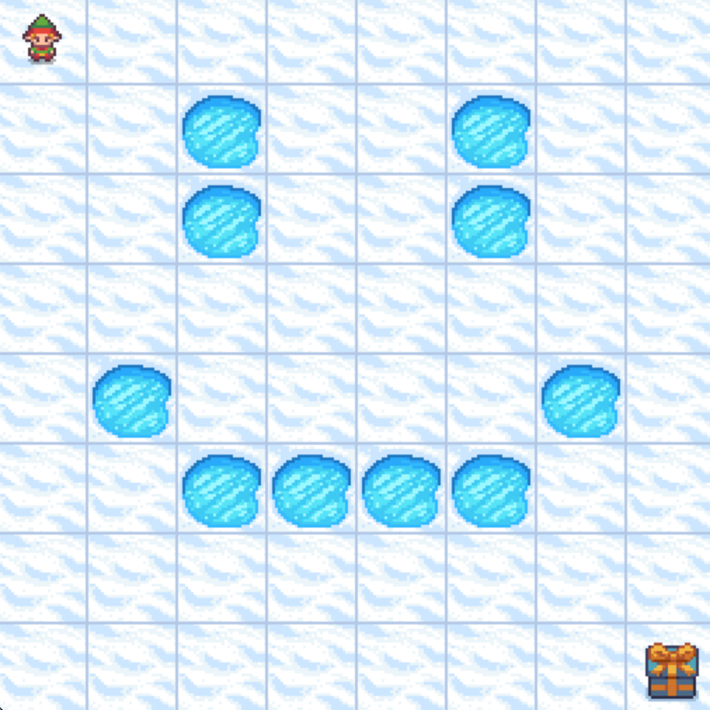
A smiley lake (Image taken by author, made using OpenAI Gymnasium’s Frozen Lake environment)
Let’s explore reinforcement learning by comparing it to familiar examples from everyday life.
Card Game — Imagine playing a card game: When you first learn the game, the rules may be unclear. The cards you play might not be the most optimal and the strategies you use might be imperfect. As you play more and maybe win a few games, you learn what cards to play when and what strategies are better than others. Sometimes it’s better to bluff, but other times you should probably fold; saving a wild card for later use might be better than playing it immediately. Knowing what the optimal course of action is learned through a combination of experience and reward. Your experience comes from playing the game and you get rewarded when your strategies work well, perhaps leading to a victory or new high score.
A game of solitaire (Image taken by author from Google’s solitaire game)
Classical Conditioning — By ringing a bell before he fed a dog, Ivan Pavlov demonstrated the connection between external stimulus and a physiological response. The dog was conditioned to associate the sound of the bell with being fed and thus began to drool at the sound of the bell, even when no food was present. Though not strictly an example of reinforcement learning, through repeated experiences where the dog was rewarded with food at the sound of the bell, it still learned to associate the two together.
Feedback Control — An application of control theory found in engineering disciplines where a system’s behaviour can be adjusted by providing feedback to a controller. As a subset of feedback control, reinforcement learning requires feedback from our current environment to influence our actions. By providing feedback in the form of reward, we can incentivize our agent to pick the optimal course of action.
The Agent, State, and Environment
Reinforcement learning is a learning process built on the accumulation of past experiences coupled with quantifiable reward. In each example, we illustrate how our experiences can influence our actions and how reinforcing a positive association between reward and response could potentially be used to solve certain problems. If we can learn to associate reward with an optimal action, we could derive an algorithm that will select actions that yield the highest probable reward.
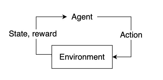
In reinforcement learning, the “learner” is called the agent. The agent interacts with our environment and, through its actions, learns what is considered “good” or “bad” based on the reward it receives.
The feedback cycle in reinforcement learning: Agent -> Action -> Environment -> Reward, State (Image by author)
To select a course of action, our agent needs some information about our environment, given by the state. The state represents current information about the environment, such as position, velocity, time, etc. Our agent does not necessarily know the entirety of the current state. The information available to our agent at any given point in time is referred to as an observation, which contains some subset of information present in the state. Not all states are fully observable, and some states may require the agent to proceed knowing only a small fraction of what might actually be happening in the environment. Using the observation, our agent must infer what the best possible action might be based on learned experience and attempt to select the action that yields the highest expected reward.
After selecting an action, the environment will then respond by providing feedback in the form of an updated state and reward. This reward will help us determine if the action the agent took was optimal or not.
Markov Decision Processes (MDPs)
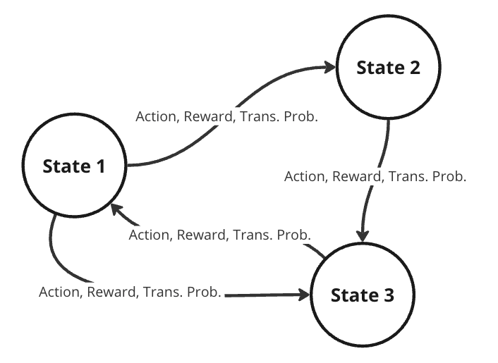
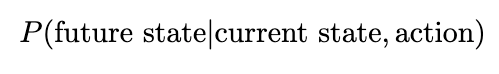
To better represent this problem, we might consider it as a Markov decision process (MDP). A MDP is a directed graph where each edge in the graph has a non-deterministic property. At each possible state in our graph, we have a set of actions we can choose from, with each action yielding some fixed reward and having some transitional probability of leading to some subsequent state. This means that the same actions are not guaranteed to lead to the same state every time since the transition from one state to another is not only dependent on the action, but the transitional probability as well.
Representation of a Markov decision process (Image by author)
Randomness in decision models is useful in practical RL, allowing for dynamic environments where the agent lacks full control. Turn-based games like chess require the opponent to make a move before you can go again. If the opponent plays randomly, the future state of the board is never guaranteed, and our agent must play while accounting for a multitude of different probable future states. When the agent takes some action, the next state is dependent on what the opponent plays and is therefore defined by a probability distribution across possible moves for the opponent.
Animation showcasing that the state of the chess board is also dependent on what moves the opponent chooses to play (Image by author)
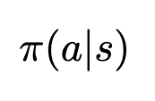
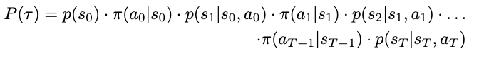
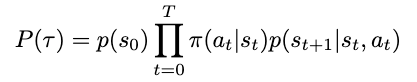
Our future state is therefore a function of both the probability of the agent selecting some action and the transitional probability of the opponent selecting some action. In general, we can assume that for any environment, the probability of our agent moving to some subsequent state from our current state is denoted by the joint probability of the agent selecting some action and the transitional probability of moving to that state.
Solving the MDP
To determine the optimal course of action, we want to provide our agent with lots of experience. Through repeated iterations of our environment, we aim to give the agent enough feedback that it can correctly choose the optimal action most, if not all, of the time. Recall our definition of reinforcement learning: a learning process built on the accumulation of past experiences coupled with quantifiable reward. After accumulating some experience, we want to use this experience to better select our future actions.
We can quantify our experiences by using them to predict the expected reward from future states. As we accumulate more experience, our predictions will become more accurate, converging to the true value after a certain number of iterations. For each reward that we receive, we can use that to update some information about our state, so the next time we encounter this state, we’ll have a better estimate of the reward that we might expect to receive.
Frozen Lake Problem
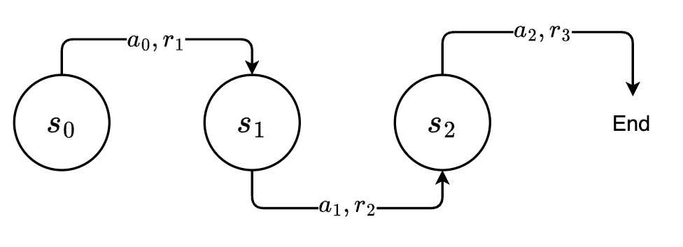
Let’s consider consider a simple environment where our agent is a small character trying to navigate across a frozen lake, represented as a 2D grid. It can move in four directions: down, up, left, or right. Our goal is to teach it to move from its start position at the top left to an end position located at the bottom right of the map while avoiding the holes in the ice. If our agent manages to successfully reach its destination, we’ll give it a reward of +1. For all other cases, the agent will receive a reward of 0, with the added condition that if it falls into a hole, the exploration will immediately terminate.
Each state can be denoted by its coordinate position in the grid, with the start position in the top left denoted as the origin (0, 0), and the bottom right ending position denoted as (3, 3).
The most generic solution would be to apply some pathfinding algorithm to find the shortest path to from top left to bottom right while avoiding holes in the ice. However, the probability that the agent can move from one state to another is not deterministic. Each time the agent tries to move, there is a 66% chance that it will “slip” and move to a random adjacent state. In other words, there is only a 33% chance of the action the agent chose actually occurring. A traditional pathfinding algorithm cannot handle the introduction of a transitional probability. Therefore, we need an algorithm that can handle stochastic environments, aka reinforcement learning.
This problem can easily be represented as a MDP, with each state in our grid having some transitional probability of moving to any adjacent state. To solve our MDP, we need to find the optimal course of action from any given state. Recall that if we can find a way to accurately predict the future rewards from each state, we can greedily choose the best possible path by selecting whichever state yields the highest expected reward. We will refer to this predicted reward as the state-value. More formally, the state-value will define the expected reward gained starting from some state plus an estimate of the expected rewards from all future states thereafter, assuming we act according to the same policy of choosing the highest expected reward. Initially, our agent will have no knowledge of what rewards to expect, so this estimate can be arbitrarily set to 0.
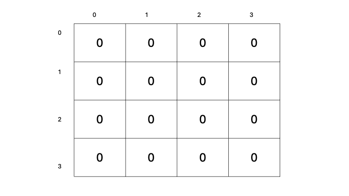
Let’s now define a way for us to select actions for our agent to take: We’ll begin with a table to store our predicted state-value estimates for each state, containing all zeros.
Table denoting the estimated state-value for each state in our grid (Image by author)
Our goal is to update these state-value estimates as we explore our environment. The more we traverse our environment, the more experience we will have, and the better our estimates will become. As our estimates improve, our state-values will become more accurate, and we will have a better representation of which states yield a higher reward, therefore allowing us to select actions based on which subsequent state has the highest state-value. This will surely work, right?
Visual representation of a single branch of our MDP (Image by author)
State-value vs. Action-value
Nope, sorry. One immediate problem that you might notice is that simply selecting the next state based on the highest possible state-value isn’t going to work. When we look at the set of possible next states, we aren’t considering our current action—that is, the action that we will take from our current state to get to the next one. Based on our definition of reinforcement learning, the agent-environment feedback loop always consists of the agent taking some action and the environment responding with both state and reward. If we only look at the state-values for possible next states, we are considering the reward that we would receive starting from those states, which completely ignores the action (and consequent reward) we took to get there. Additionally, trying to select a maximum across the next possible states assumes we can even make it there in the first place. Sometimes, being a little more conservative will help us be more consistent in reaching the end goal; however, this is out of the scope of this article :(.
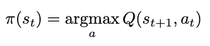
Instead of evaluating across the set of possible next states, we’d like to directly evaluate our available actions. If our previous state-value function consisted of the expected rewards starting from the next state, we’d like to update this function to now include the reward from taking an action from the current state to get to the next state, plus the expected rewards from there on. We’ll call this new estimate that includes our current action action-value.
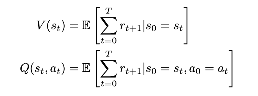
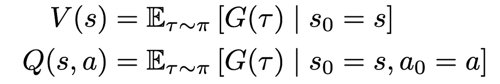
We can now formally define our state-value and action-value functions based on rewards and transitional probability. We’ll use expected value to represent the relationship between reward and transitional probability. We’ll denote our state-value as V and our action-value as Q, based on standard conventions in RL literature.
Equations for state- and action-value (Image by author)
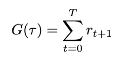
The state-value V of some state s[t] is the expected sum of rewards r[t] at each state starting from s[t] to some future state s[T]; the action-value Q of some state s[t] is the expected sum of rewards r[t] at each state starting by taking an action a[t] to some future state-action pair s[T], a[T].
This definition is actually not the most accurate or conventional, and we’ll improve on it later. However, it serves as a general idea of what we’re looking for: a quantitative measure of future rewards.
Our state-value function V is an estimate of the maximum sum of rewards r we would obtain starting from state s and continually moving to the states that give the highest reward. Our action-value function is an estimate of the maximum reward we would obtain by taking action from some starting state and continually choosing the optimal actions that yield the highest reward thereafter. In both cases, we choose the optimal action/state to move to based on the expected reward that we would receive and loop this process until we either fall into a hole or reach our goal.
Greedy Policy & Return
The method by which we choose our actions is called a policy. The policy is a function of state—given some state, it will output an action. In this case, since we want to select the next action based on maximizing the rewards, our policy can be defined as a function returning the action that yields the maximum action-value (Q-value) starting from our current state, or an argmax. Since we’re always selecting a maximum, we refer to this particular policy as greedy. We’ll denote our policy as a function of state s: π(s), formally defined as
Equation for the policy function = the action that yields the maximum estimated Q-value from some state s (Image by author)
To simplify our notation, we can also define a substitution for our sum of rewards, which we’ll call return, and a substitution for a sequence of states and actions, which we’ll call a trajectory. A trajectory, denoted by the Greek letter τ (tau), is denoted as
Notation for trajectory: defined as some sequence of state-action pairs until some future timestep T. Defining the trajectory allows us to skip writing the entire sequence of states and actions, and substitute a single variable instead :P! (Image by author)
Since our environment is stochastic, it’s important to also consider the likelihood of such a trajectory occurring — low probability trajectories will reduce the expectation of reward. (Since our expected value consists of multiplying our reward by the transitional probability, trajectories that are less likely will have a lower expected reward compared to high probability ones.) The probability can be derived by considering the probability of each action and state happening incrementally: At any timestep in our MDP, we will select actions based on our policy, and the resulting state will be dependent on both the action we selected and the transitional probability. Without loss of generality, we’ll denote the transitional probability as a separate probability distribution, a function of both the current state and the attempted action. The conditional probability of some future state occurring is therefore defined as
Transitional probability of moving to a future state from a current state — for our frozen lake though, we know this value is fixed at ~0.33 (Image by author)
And the probability of some action happening based on our policy is simply evaluated by passing our state into our policy function
Expression for the probability of some action being selected by the policy given some state (Image by author)
Our policy is currently deterministic, as it selects actions based on the highest expected action-value. In other words, actions that have a low action-value will never be selected, while actions with a high Q-value will always be selected. This results in a Bernoulli distribution across possible actions. This is very rarely beneficial, as we’ll see later.
Applying these expressions to our trajectory, we can define the probability of some trajectory occurring as
Expanded equation for the probability of a certain trajectory occurring. Note that the probability of s0 is fixed at 1 assuming we start from the same state (top left) every time. (Image by author)
For clarity, here’s the original notation for a trajectory:
Notation for trajectory: defined as some sequence of state-action pairs until some future timestep T (Image by author)
More concisely, we have
Concise notation for the probability of a trajectory occurring (Image by author)
Defining both the trajectory and its probability allows us to substitute these expressions to simplify our definitions for both return and its expected value. The return (sum of rewards), which we’ll define as G based on conventions, can now be written as
Equation for return (Image by author)
We can also define the expected return by introducing probability into the equation. Since we’ve already defined the probability of a trajectory, the expected return is therefore
Updated equation for expected return = the probability of the trajectory occurring times the return (Image by author)
We can now adjust the definition of our value functions to include the expected return
Updated equations for state- and action-value (Image by author)
The main difference here is the addition of the subscript τ∼π indicating that our trajectory was sampled by following our policy (ie. our actions are selected based on the maximum Q-value). We’ve also removed the subscript t for clarity. Here’s the previous equation again for reference:
Equations for state- and action-value (Image by author)
Discounted Return
So now we have a fairly well-defined expression for estimating return but before we can start iterating through our environment, there’s still some more things to consider. In our frozen lake, it’s fairly unlikely that our agent will continue to explore indefinitely. At some point, it will slip and fall into a hole, and the episode will terminate. However, in practice, RL environments might not have clearly defined endpoints, and training sessions might go on indefinitely. In these situations, given an indefinite amount of time, the expected return would approach infinity, and evaluating the state- and action-value would become impossible. Even in our case, setting a hard limit for computing return is oftentimes not beneficial, and if we set the limit too high, we could end up with pretty absurdly large numbers anyway. In these situations, it is important to ensure that our reward series will converge using a discount factor. This improves stability in the training process and ensures that our return will always be a finite value regardless of how far into the future we look. This type of discounted return is also referred to as infinite horizon discounted return.
To add discounting to our return equation, we’ll introduce a new variable γ (gamma) to represent the discount factor.
Equation for discounted return (Image by author)
Gamma must always be less than 1, or our series will not converge. Expanding this expression makes this even more apparent
Expanded equation for discounted return (Image by author)
We can see that as time increases, gamma will be raised to a higher and higher power. As gamma is less than 1, raising it to a higher exponent will only make it smaller, thus exponentially decreasing the contribution of future rewards to the overall sum. We can substitute this updated definition of return back into our value functions, though nothing will visibly change since the variable is still the same.
Equations for state- and action-value, copied again for emphasis (Image by author)
Exploration vs. Exploitation
We mentioned earlier that always being greedy is not the best choice. Always selecting our actions based on the maximum Q-value will probably give us the highest chance of maximizing our reward, but that only holds when we have accurate estimates of those Q-values in the first place. To obtain accurate estimates, we need a lot of information, and we can only gain information by trying new things — that is, exploration.
When we select actions based on the highest estimated Q-value, we exploit our current knowledge base: we leverage our accumulated experiences in an attempt to maximize our reward. When we select actions based on any other metric, or even randomly, we explore alternative possibilities in an attempt to gain more useful information to update our Q-value estimates with. In reinforcement learning, we want to balance both exploration and exploitation. To properly exploit our knowledge, we need to have knowledge, and to gain knowledge, we need to explore.
Epsilon-Greedy Policy
We can balance exploration and exploitation by changing our policy from purely greedy to an epsilon-greedy one. An epsilon-greedy policy acts greedily most of the time with a probability of 1- ε, but has a probability of ε to act randomly. In other words, we’ll exploit our knowledge most of the time in an attempt to maximize reward, and we’ll explore occasionally to gain more knowledge. This is not the only way of balancing exploration and exploitation, but it is one of the simplest and easiest to implement.
Summary
Now the we’ve established a basis for understanding RL principles, we can move to discussing the actual algorithm — which will happen in the next article. For now, we’ll go over the high-level overview, combining all these concepts into a cohesive pseudo-code which we can delve into next time.
Q-Learning
The focus of this article was to establish the basis for understanding and implementing Q-learning. Q-learning consists of the following steps:
Initialize a tabular estimate of all action-values (Q-values), which we update as we iterate through our environment.
Select an action by sampling from our epsilon-greedy policy.
Collect the reward (if any) and update our estimate for our action-value.
Move to the next state, or terminate if we fall into a hole or reach the goal.
Loop steps 2–4 until our estimated Q-values converge.
Q-learning is an iterative process where we build estimates of action-value (and expected return), or “experience”, and use our experiences to identify which actions are the most rewarding for us to choose. These experiences are “learned” over many successive iterations of our environment and by leveraging them we will be able to consistently reach our goal, thus solving our MDP.
Glossary
Environment — anything that cannot be arbitrarily changed by our agent, aka the world around it
State — a particular condition of the environment
Observation — some subset of information from the state
Policy — a function that selects an action given a state
Agent — our “learner” which acts according to a policy in our environment
Reward — what our agent receives after performing certain actions
Return — a sum of rewards across a series of actions
Discounting — the process through which we ensure that our return does not reach infinity
State-value — the expected return starting from a state and continuing to act according to some policy, forever
Action-value — the expected return starting from a state and taking some action, and then continuing to act according to some policy, forever
Trajectory — a series of states and actions
Markov Decision Process (MDP) — the model we use to represent decision problems in RL aka a directed graph with non-deterministic edges
Exploration — how we obtain more knowledge
Exploitation — how we use our existing knowledge base to gain more reward
Q-Learning — a RL algorithm where we iteratively update Q-values to obtain better estimates of which actions will yield higher expected return
Reinforcement Learning — a learning process built on the accumulation of past experiences coupled with quantifiable reward
If you’ve read this far, consider leaving some feedback about the article — I’d appreciate it ❤.
References
[1] Gymnasium, Frozen Lake (n.d.), OpenAI Gymnasium Documentation.
Building real-world skills through hands-on trial and error.
The engaging discussions sparked by my recent blog post, “We Need to Raise the Bar for AI Product Managers,” highlighted a shared passion for advancing the field of AI product management. Many current and aspiring PMs have since reached out, asking how they can learn more about AI on their path to becoming an AI product manager.
In my experience, the most effective AI PMs excel in two key areas: identifying opportunities where AI can add value, and working with model developers to deploy the technology effectively. This requires a solid understanding of how different kinds of models are likely to behave when they go live — a reality that often surprises newcomers. The gap between flashy demos or early-stage prototypes and actual product performance can be substantial, whether you’re dealing with customer-facing applications or backend data pipelines that power products.
The best way to develop this intuition is by deploying a range of models into products and making plenty of mistakes along the way. The next best thing is to explore what other teams at your company are doing and learn from their mistakes (and triumphs). Dig up any documentation you can find and, where possible, listen in on product reviews or team updates. Often, people who worked directly on the projects will be happy to chat, answer your questions, and provide more context, especially if your team might be considering anything similar.
But what if you aren’t working at a company doing anything with AI? Or your company is focused on a very narrow set of technologies? Or maybe you’re in the midst of a job search?
In addition to checking out resources to familiarize yourself with terminology and best practices, I recommend developing your own AI projects. I actually recommend side projects even if you can learn a lot from your day job. Every AI use case has its own nuances, and the more examples you can get close to, the faster you’ll develop an intuition about what does and doesn’t work.
For a starter project, I recommend starting with LLMs like Claude or ChatGPT. You should be able to get something substantial up and running in a matter of hours (minutes if you already know how to code and write effective prompts). While not all AI projects at a real company will use LLMs, they are gaining significant traction. More importantly, it’s much easier to create your own working model with only rudimentary data science or coding knowledge. If your coding skills are rusty, using the developer APIs will give you a chance to brush up, and if you get stuck the LLM is a great resource to help with both code generation and troubleshooting. If you’re new to both coding and LLMs, then using the online chat interface is a great way to warm up.
Characteristics of a Good Starter Project
But what’s the difference between using the ChatGPT website or app to make you more productive (with requests like summarizing an article or drafting an email) versus an actual project?
A project should aim to solve a real problem in a repeatable way. It’s these nuances that will help you hone some of the most important skills for AI product management work at a company, especially model evaluation. Check out my article “What Exactly is an Eval and Why Should Product Managers Care” for an overview of model evaluation basics.
To ensure what you’re working on is a real project that can have its own mini eval, make sure you have:
Multiple test samples: Aim for projects where you can evaluate the model on at least 20 different examples or data points.
Diverse data: Ensure your dataset includes a variety of scenarios to test what causes the model to break (thus giving you more chances to fix it).
Clear evaluation criteria: Be clear from the start how an effective model or product behaves. You should have 20 ideal responses for your 20 examples to score the model.
Real-world relevance: Choose a problem that reflects actual use cases in your work, your personal life, or for someone close to you. You need to be well-informed to evaluate the model’s efficacy.
Sample Project Ideas
Please don’t do these specific projects unless one of them really speaks to you. These are for illustrative purposes only to help convey what makes a real project, versus a one-off query:
Gift Recommendation Classifier
Goal: Decide if a given product would be a good gift for an opinionated friend or family member.
Method: Use text generation to evaluate product titles and descriptions with a prompt describing the recipient’s taste profile. If you want to go a little more complex you could use vision capabilities to evaluate the product description and title AND a product image.
Test samples: 50 different product images and descriptions. To make this tricky, your examples should include some products that are obviously bad, some that obviously good, many that are borderline, and some that are completely random.
Evaluation: Have the target gift recipient evaluate the list of products, rating each on a scale (ex: “no way”, “meh” and “hell yes”) for how well it matches their preferences. Compare these ratings to the model’s classifications. You can also learn a lot from asking the model to give you a justification for why it thinks each item would or wouldn’t be a good match. This will help you troubleshoot failures and guide prompt updates, plus they will teach you a lot about how LLMs “think”.
Recipe Book Digitization
Goal: Convert your grandmother’s favorite out-of-print recipe book into an app for you and your cousins.
Method: Use vision capabilities to extract recipes from photos of the pages in a recipe book.
Test samples: 20 images of different types of recipes. To make it simpler to start, you could just focus on desserts. The examples might include 3 kinds of cookies, 4 kinds of cake, etc.
Evaluation: Are all the key ingredients and instructions from each included in the final output? Carefully compare the LLM output to the original recipe, checking for accuracy in ingredients, measurements, and cooking instructions. Bonus points if you can get the final data into some kind of structured format (e.g., JSON or CSV) for easier use in an app.
Image generated by the author using Midjourney
Public Figure Quote Extractor
Goal: Help a public figure’s publicity team identify any quote or fact said by them for your fact-checking team to verify.
Method: Use text generation to evaluate the text of articles and return a list of quotes and facts about your public figure mentioned in each article.
Test samples: 20 recent articles about the public figure covering at least 3 different events from at least 4 different publications (think one gossip site, one national paper like the New York Times, and something in between like Politico)
Evaluation: Read each article carefully and see if any facts or quotes from the public figure were missed. Imagine your job could be on the line if your summarizer hallucinates (ex: saying they said something they didn’t) or misses a key piece of misinformation. Check that all the quotes and facts the summarizer found are in fact related to your public figure, and also that they are all mentioned in the article.
You’re welcome to use any LLM for these projects, but in my experience, the ChatGPT API is the easiest to get started with if you have limited coding experience. Once you’ve successfully completed one project, evaluating another LLM on the same data is relatively straightforward.
Remember, the goal of starter projects isn’t perfection but to find an interesting project with some complexity to ensure you encounter difficulties. Learning to troubleshoot, iterate, and even hit walls where you realize something isn’t possible will help you hone your intuition for what is and isn’t feasible, and how much work is involved.
Embrace the learning process
Developing a strong intuition for AI capabilities and limitations is crucial for effective AI product management. By engaging in hands-on projects, you’ll gain invaluable experience in model evaluation, troubleshooting, and iteration. This practical knowledge will make you a more effective partner to model developers, enabling you to:
Identify areas where AI can truly add value
Make realistic estimates for AI project timelines and resourcing requirements
Contribute meaningfully to troubleshooting and evaluation processes
As you tackle these projects, you’ll develop a nuanced understanding of AI’s real-world applications and challenges. This experience will set you apart in the rapidly evolving field of AI product management, preparing you to lead innovative projects and make informed decisions that drive product success.
Remember, the journey to becoming an expert AI PM is ongoing. Embrace the learning process, stay curious, and continually seek out new challenges to refine your skills. With dedication and hands-on experience, you’ll be well-equipped to navigate the exciting frontier of AI product development.
Have questions about your AI project or this article? Connect with me on LinkedIn to continue the conversation.
Clustering is a must-have skill set for any data scientist due to its utility and flexibility to real-world problems. This article is an overview of clustering and the different types of clustering algorithms.
What is Clustering?
Clustering is a popular unsupervised learning technique that is designed to group objects or observations together based on their similarities. Clustering has a lot of useful applications such as market segmentation, recommendation systems, exploratory analysis, and more.
Image by Author
While clustering is a well-known and widely used technique in the field of data science, some may not be aware of the different types of clustering algorithms. While there are just a few, it is important to understand these algorithms and how they work to get the best results for your use case.
Centroid-Based Clustering
Centroid-based clustering is what most think of when it comes to clustering. It is the “traditional” way to cluster data by using a defined number of centroids (centers) to group data points based on their distance to each centroid. The centroid ultimately becomes the mean of it’s assigned data points. While centroid-based clustering is powerful, it is not robust against outliers, as outliers will need to be assigned to a cluster.
K-Means
K-Means is the most widely used clustering algorithm, and is likely the first one you will learn as a data scientist. As explained above, the objective is to minimize the sum of distances between the data points and the cluster centroid to identify the correct group that each data point should belong to. Here’s how it works:
A defined number of centroids are randomly dropped into the vector space of the unlabeled data (initialization).
Each data point measures itself to each centroid (usually using Euclidean distance) and assigns itself to the closest one.
The centroids relocate to the mean of their assigned data points.
Steps 2–3 repeat until the ‘optimal’ clusters are produced.
Image by Author
from sklearn.cluster import KMeans import numpy as np
#sample data X = np.array([[1, 2], [1, 4], [1, 0], [10, 2], [10, 4], [10, 0]])
#print the results, use to predict, and print centers kmeans.labels_ kmeans.predict([[0, 0], [12, 3]]) kmeans.cluster_centers_
K-Means ++
K-Means ++ is an improvement of the initialization step of K-Means. Since the centroids are randomly dropped in, there is a chance that more than one centroid might be initialized into the same cluster, resulting in poor results.
However K-Means ++ solves this by randomly assigning the first centroid that will eventually find the largest cluster. Then, the other centroids are placed a certain distance away from the initial cluster. The goal of K-Means ++ is to push the centroids as far as possible from one another. This results in high-quality clusters that are distinct and well-defined.
from sklearn.cluster import KMeans import numpy as np
#sample data X = np.array([[1, 2], [1, 4], [1, 0], [10, 2], [10, 4], [10, 0]])
#print the results, use to predict, and print centers kmeans.labels_ kmeans.predict([[0, 0], [12, 3]]) kmeans.cluster_centers_
Density-Based Clustering
Density-based algorithms are also a popular form of clustering. However, instead of measuring from randomly placed centroids, they create clusters by identifying high-density areas within the data. Density-based algorithms do not require a defined number of clusters, and therefore are less work to optimize.
While centroid-based algorithms perform better with spherical clusters, density-based algorithms can take arbitrary shapes and are more flexible. They also do not include outliers in their clusters and therefore are robust. However, they can struggle with data of varying densities and high dimensions.
Image by Author
DBSCAN
DBSCAN is the most popular density-based algorithm. DBSCAN works as follows:
DBSCAN randomly selects a data point and checks if it has enough neighbors within a specified radius.
If the point has enough neighbors, it is marked as part of a cluster.
DBSCAN recursively checks if the neighbors also have enough neighbors within the radius until all points in the cluster have been visited.
Repeat steps 1–3 until the remaining data point do not have enough neighbors in the radius.
Remaining data points are marked as outliers.
from sklearn.cluster import DBSCAN
import numpy as np

#sample data
X = np.array([[1, 2], [2, 2], [2, 3],
              [8, 7], [8, 8], [25, 80]])

#create model
clustering = DBSCAN(eps=3, min_samples=2).fit(X)

#print results
clustering.labels_
Hierarchical Clustering
Next, we have hierarchical clustering. This method starts off by computing a distance matrix from the raw data. This distance matrix is best and often visualized by a dendrogram (see below). Data points are linked together one by one by finding the nearest neighbor to eventually form one giant cluster. Therefore, a cut-off point to identify the clusters by stopping all data points from linking together.
Image by Author
By using this method, the data scientist can build a robust model by defining outliers and excluding them in the other clusters. This method works great against hierarchical data, such as taxonomies. The number of clusters depends on the depth parameter and can be anywhere from 1-n.
from scipy.cluster.hierarchy import dendrogram, linkage from sklearn.cluster import AgglomerativeClustering from scipy.cluster.hierarchy import fcluster
Lastly, distribution-based clustering considers a metric other than distance and density, and that is probability. Distribution-based clustering assumes that the data is made up of probabilistic distributions, such as normal distributions. The algorithm creates ‘bands’ that represent confidence intervals. The further away a data point is from the center of a cluster, the less confident we are that the data point belongs to that cluster.
Image by Author
Distribution-based clustering is very difficult to implement due to the assumptions it makes. It usually is not recommended unless rigorous analysis has been done to confirm its results. For example, using it to identify customer segments in a marketing dataset, and confirming these segments follow a distribution. This can also be a great method for exploratory analysis to see not only what the centers of clusters comprise of, but also the edges and outliers.
Conclusion
Clustering is an unsupervised machine learning technique that has a growing utility in many fields. It can be used to support data analysis, segmentation projects, recommendation systems, and more. Above we have explored how they work, their pros and cons, code samples, and even some use cases. I would consider experience with clustering algorithms a must-have for data scientists due to their utility and flexibility.
I hope you have enjoyed my article! Please feel free to comment, ask questions, or request other topics.
We use cookies on our website to give you the most relevant experience by remembering your preferences and repeat visits. By clicking “Accept”, you consent to the use of ALL the cookies.
This website uses cookies to improve your experience while you navigate through the website. Out of these, the cookies that are categorized as necessary are stored on your browser as they are essential for the working of basic functionalities of the website. We also use third-party cookies that help us analyze and understand how you use this website. These cookies will be stored in your browser only with your consent. You also have the option to opt-out of these cookies. But opting out of some of these cookies may affect your browsing experience.
Necessary cookies are absolutely essential for the website to function properly. These cookies ensure basic functionalities and security features of the website, anonymously.
Cookie
Duration
Description
cookielawinfo-checkbox-analytics
11 months
This cookie is set by GDPR Cookie Consent plugin. The cookie is used to store the user consent for the cookies in the category "Analytics".
cookielawinfo-checkbox-functional
11 months
The cookie is set by GDPR cookie consent to record the user consent for the cookies in the category "Functional".
cookielawinfo-checkbox-necessary
11 months
This cookie is set by GDPR Cookie Consent plugin. The cookies is used to store the user consent for the cookies in the category "Necessary".
cookielawinfo-checkbox-others
11 months
This cookie is set by GDPR Cookie Consent plugin. The cookie is used to store the user consent for the cookies in the category "Other.
cookielawinfo-checkbox-performance
11 months
This cookie is set by GDPR Cookie Consent plugin. The cookie is used to store the user consent for the cookies in the category "Performance".
viewed_cookie_policy
11 months
The cookie is set by the GDPR Cookie Consent plugin and is used to store whether or not user has consented to the use of cookies. It does not store any personal data.
Functional cookies help to perform certain functionalities like sharing the content of the website on social media platforms, collect feedbacks, and other third-party features.
Performance cookies are used to understand and analyze the key performance indexes of the website which helps in delivering a better user experience for the visitors.
Analytical cookies are used to understand how visitors interact with the website. These cookies help provide information on metrics the number of visitors, bounce rate, traffic source, etc.
Advertisement cookies are used to provide visitors with relevant ads and marketing campaigns. These cookies track visitors across websites and collect information to provide customized ads.