Category: Artificial Intelligence

A gentle introduction to mechanistic interpretability through simple algorithmic examples

Introduction

This article shows how small Artificial Neural Networks (NN) can represent basic functions. The goal is to provide fundamental intuition about how NNs work and to serve as a gentle introduction to Mechanistic Interpretability — a field that seeks to reverse engineer NNs.

I present three examples of elementary functions, describe each using a simple algorithm, and show how the algorithm can be “coded” into the weights of a neural network. Then, I explore if the network can learn the algorithm using backpropagation. I encourage readers to think about each example as a riddle and take a minute before reading the solution.

Machine Learning Topology

This article attempts to break NNs into discrete operations and describe them as algorithms. An alternative approach, perhaps more common and natural, is looking at the continuous topological interpretations of the linear transformations in different layers.

The following are some great resources for strengthening your topological intuition:

• Tensorflow Playground — a simple tool for building basic intuition on classification tasks.
• ConvnetJS Demo — a more sophisticated tool for visualizing NNs for classification tasks.
• Neural Networks, Manifolds, and Topology — a great article for building topological intuition of how NNs work.

Three Elementary Functions

In all the following examples, I use the terminology “neuron” for a single node in the NN computation graph. Each neuron can be used only once (no cycles; e.g., not RNN), and it performs 3 operations in the following order:

1. Inner product with the input vector.
2. Adding a bias term.
3. Running a (non-linear) activation function.

I provide only minimal code snippets so that reading will be fluent. This Colab notebook includes the entire code.

The < operator

How many neurons are required to learn the function “x < 10”? Write an NN that returns 1 when the input is smaller than 10 and 0 otherwise.

Solution

Let’s start by creating sample dataset that follows the pattern we want to learn

X = [[i] for i in range(-20, 40)]
Y = [1 if z[0] < 10 else 0 for z in X]

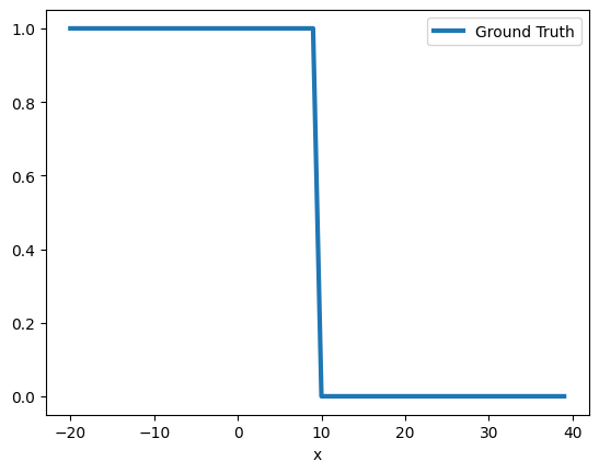
This classification task can be solved using logistic regression and a Sigmoid as the output activation. Using a single neuron, we can write the function as Sigmoid(ax+b). b, the bias term, can be thought of as the neuron’s threshold. Intuitively, we can set b = 10 and a = -1 and get F=Sigmoid(10-x)

Let’s implement and run F using PyTorch

model = nn.Sequential(nn.Linear(1,1), nn.Sigmoid())
d = model.state_dict()
d["0.weight"] = torch.tensor([[-1]]).float()
d['0.bias'] = torch.tensor([10]).float()
model.load_state_dict(d)
y_pred = model(x).detach().reshape(-1)

Seems like the right pattern, but can we make a tighter approximation? For example, F(9.5) = 0.62, we prefer it to be closer to 1.

For the Sigmoid function, as the input approaches -∞ / ∞ the output approaches 0 / 1 respectively. Therefore, we need to make our 10 — x function return large numbers, which can be done by multiplying it by a larger number, say 100, to get F=Sigmoid(100(10-x)), now we’ll get F(9.5) =~1.

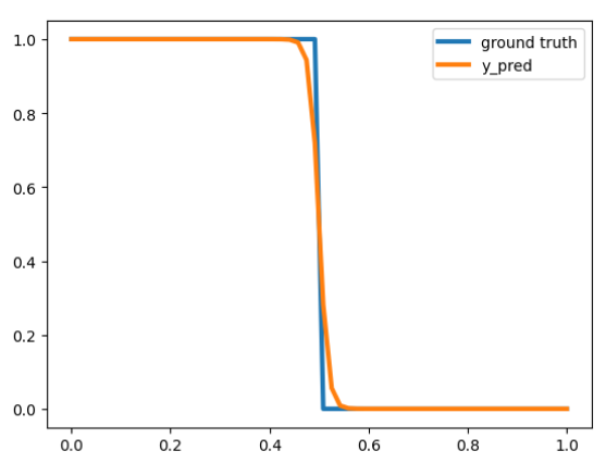
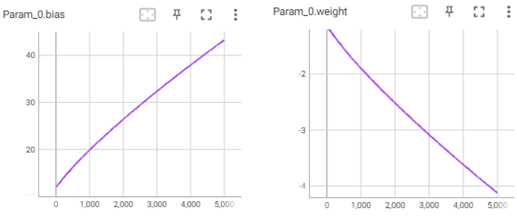
Indeed, when training a network with one neuron, it converges to F=Sigmoid(M(10-x)), where M is a scalar that keeps growing during training to make the approximation tighter.

To clarify, our single-neuron model is only an approximation of the “<10” function. We will never be able to reach a loss of zero, because the neuron is a continuous function while “<10” is not a continuous function.

Min(a, b)

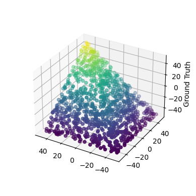
Write a neural network that takes two numbers and returns the minimum between them.

Solution

Like before, let’s start by creating a test dataset and visualizing it

X_2D = [
[random.randrange(-50, 50),
 random.randrange(-50, 50)]
 for i in range(1000)
]
Y = [min(a, b) for a, b in X_2D]

In this case, ReLU activation is a good candidate because it is essentially a maximum function (ReLU(x) = max(0, x)). Indeed, using ReLU one can write the min function as follows

min(a, b) = 0.5 (a + b -|a - b|) = 0.5 (a + b - ReLU(b - a) - ReLU(a - b))

[Equation 1]

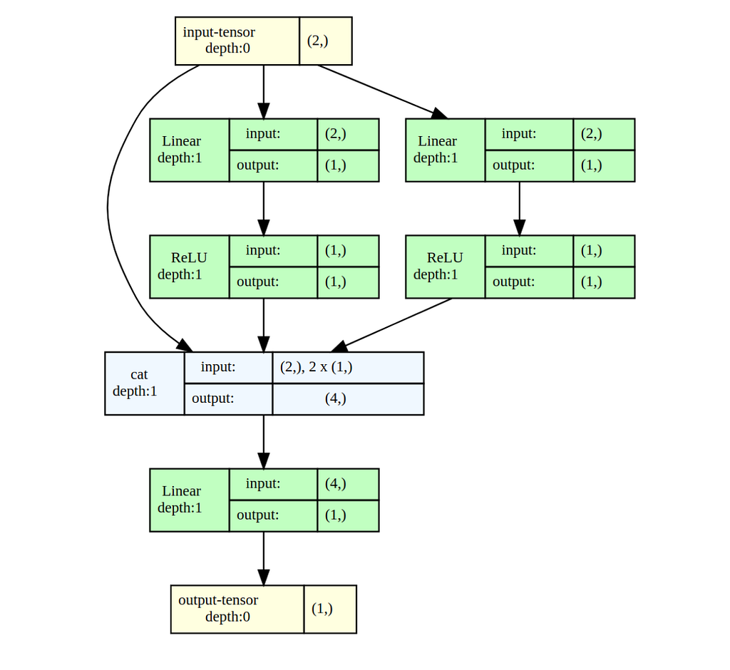
Now let’s build a small network that is capable of learning Equation 1, and try to train it using gradient descent

class MinModel(nn.Module):
  def __init__(self):
      super(MinModel, self).__init__()

      # For ReLU(a-b)
      self.fc1 = nn.Linear(2, 1)
      self.relu1 = nn.ReLU()
      # For ReLU(b-a)
      self.fc2 = nn.Linear(2, 1)
      self.relu2 = nn.ReLU()
      # Takes 4 inputs
      # [a, b, ReLU(a-b), ReLU(b-a)]
      self.output_layer = nn.Linear(4, 1)

  def forward(self, x):
      relu_output1 = self.relu1(self.fc1(x))
      relu_output2 = self.relu2(self.fc2(x))
      return self.output_layer(
          torch.cat(
             (x, Relu_output1, relu_output2),
             dim=-1
          )
      )

Training for 300 epochs is enough to converge. Let’s look at the model’s parameters

>> for k, v in model.state_dict().items():
>>   print(k, ": ", torch.round(v, decimals=2).numpy())

fc1.weight :  [[-0. -0.]]
fc1.bias :  [0.]
fc2.weight :  [[ 0.71 -0.71]]
fc2.bias :  [-0.]
output_layer.weight :  [[ 1.    0.    0.   -1.41]]
output_layer.bias :  [0.]

Many weights are zeroing out, and we are left with the nicely looking

model([a,b]) = a - 1.41 * 0.71 ReLU(a-b) ≈ a - ReLU(a-b)

This is not the solution we expected, but it is a valid solution and even cleaner than Equation 1! By looking at the network we learned a new nicely looking formula! Proof:

Proof:

• If a <= b: model([a,b]) = a — ReLU(a-b) = a — 0 = a
• If a > b: a — ReLU(a-b) = a — (a-b) = b

Is even?

Create a neural network that takes an integer x as an input and returns x mod 2. That is, 0 if x is even, 1 if x is odd.

This one looks quite simple, but surprisingly it is impossible to create a finite-size network that correctly classifies each integer in (-∞, ∞) (using a standard non-periodic activation function such as ReLU).

Theorem: is_even needs at least log neurons

A network with ReLU activations requires at least n neurons to correctly classify each of 2^n consecutive natural numbers as even or odd (i.e., solving is_even).

Proof: Using Induction

Base: n == 2: Intuitively, a single neuron (of the form ReLU(ax + b)), cannot solve S = [i + 1, i + 2, i + 3, i + 4] as it is not linearly separable. For example, without loss of generality, assume a > 0 and i + 2 is even. If ReLU(a(i + 2) + b) = 0, then also ReLU(a(i + 1) + b) = 0 (monotonic function), but i + 1 is odd.
More details are included in the classic Perceptrons book.

Assume for n, and look at n+1: Let S = [i + 1, …, i + 2^(n + 1)], and assume, for the sake of contradiction, that S can be solved using a network of size n. Take an input neuron from the first layer f(x) = ReLU(ax + b), where x is the input to the network. WLOG a > 0. Based on the definition of ReLU there exists a j such that:
S’ = [i + 1, …, i + j], S’’ = [i + j + 1, …, i + 2^(n + 1)]
f(x ≤ i) = 0
f(x ≥ i) = ax + b

There are two cases to consider:

• Case |S’| ≥ 2^n: dropping f and all its edges won’t change the classification results of the network on S’. Hence, there is a network of size n-1 that solves S’. Contradiction.
• Case |S’’|≥ 2^n: For each neuron g which takes f as an input g(x) = ReLU(cf(x) + d + …) = ReLU(c ReLU(ax + b) + d + …), Drop the neuron f and wire x directly to g, to get ReLU(cax + cb + d + …). A network of size n — 1 solves S’’. Contradiction.

Logarithmic Algorithm

How many neurons are sufficient to classify [1, 2^n]? I have proven that n neurons are necessary. Next, I will show that n neurons are also sufficient.

One simple implementation is a network that constantly adds/subtracts 2, and checks if at some point it reaches 0. This will require O(2^n) neurons. A more efficient algorithm is to add/subtract powers of 2, which will require only O(n) neurons. More formally:
f_i(x) := |x — i|
f(x) := f_1∘ f_1∘ f_2 ∘ f_4∘ … ∘ f_(2^(n-1)) (|x|)

Proof:

• By definition:∀ x ϵ[0, 2^i]: f_(2^(i-1)) (x) ≤ 2^(i-1).
  I.e., cuts the interval by half.
• Recursively f_1∘ f_1∘ f_2 ∘ … ∘ f_(2^(n-1)) (|x|) ≤ 1
• For every even i: is_even(f_i(x)) = is_even(x)
• Similarly is_even(f_1( f_1(x))) = is_even(x)
• We got f(x) ϵ {0,1} and is_even(x) =is_even(f(x)). QED.

Implementation

Let’s try to implement this algorithm using a neural network over a small domain. We start again by defining the data.

X = [[i] for i in range(0, 16)]
Y = [z[0] % 2 for z in X]

Because the domain contains 2⁴ integers, we need to use 6 neurons. 5 for f_1∘ f_1∘ f_2 ∘ f_4∘ f_8, + 1 output neuron. Let’s build the network and hardwire the weights

def create_sequential_model(layers_list = [1,2,2,2,2,2,1]):
  layers = []
  for i in range(1, len(layers_list)):
      layers.append(nn.Linear(layers_list[i-1], layers_list[i]))
      layers.append(nn.ReLU())
  return nn.Sequential(*layers)

# This weight matrix implements |ABS| using ReLU neurons.
# |x-b| = Relu(-(x-b)) + Relu(x-b)
abs_weight_matrix = torch_tensor([[-1, -1],
                                  [1, 1]])
# Returns the pair of biases used for each of the ReLUs.
get_relu_bias = lambda b: torch_tensor([b, -b])

d = model.state_dict()
d['0.weight'], d['0.bias'] = torch_tensor([[-1],[1]]), get_relu_bias(8)
d['2.weight'], d['2.bias'] = abs_weight_matrix, get_relu_bias(4)
d['4.weight'], d['4.bias'] = abs_weight_matrix, get_relu_bias(2)
d['6.weight'], d['6.bias'] = abs_weight_matrix, get_relu_bias(1)
d['8.weight'], d['8.bias'] = abs_weight_matrix, get_relu_bias(1)
d['10.weight'], d['10.bias'] = torch_tensor([[1, 1]]), torch_tensor([0])
model.load_state_dict(d)
model.state_dict()

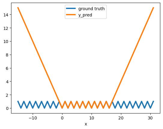
As expected we can see that this model makes a perfect prediction on [0,15]

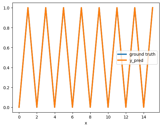
And, as expected, it doesn’t generalizes to new data points

We saw that we can hardwire the model, but would the model converge to the same solution using gradient descent?

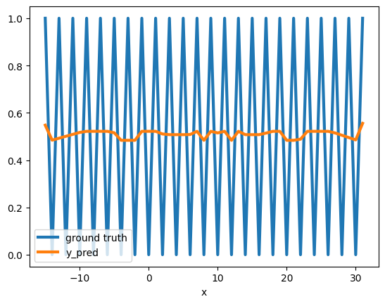
The answer is — not so easily! Instead, it is stuck at a local minimum — predicting the mean.

This is a known phenomenon, where gradient descent can get stuck at a local minimum. It is especially prevalent for non-smooth error surfaces of highly nonlinear functions (such as is_even).

More details are beyond the scope of this article, but to get more intuition one can look at the many works that investigated the classic XOR problem. Even for such a simple problem, we can see that gradient descent can struggle to find a solution. In particular, I recommend Richard Bland’s short book “Learning XOR: exploring the space of a classic problem” — a rigorous analysis of the error surface of the XOR problem.

Final Words

I hope this article has helped you understand the basic structure of small neural networks. Analyzing Large Language Models is much more complex, but it’s an area of research that is advancing rapidly and is full of intriguing challenges.

When working with Large Language Models, it’s easy to focus on supplying data and computing power to achieve impressive results without understanding how they operate. However, interpretability offers crucial insights that can help address issues like fairness, inclusivity, and accuracy, which are becoming increasingly vital as we rely more on LLMs in decision-making.

For further exploration, I recommend following the AI Alignment Forum.

*All the images were created by the author. The intro image was created using ChatGPT and the rest were created using Python libraries.

---

How Tiny Neural Networks Represent Basic Functions was originally published in Towards Data Science on Medium, where people are continuing the conversation by highlighting and responding to this story.

Open-Source Data Observability with Elementary — From Zero to Hero (Part 2)

The guide to take your dbt tests to the next level for free

In the previous part, we have set up Elementary in our dbt repository and hopefully also run it on our production. In this part, we will go more in detail and examine the available tests in Elementary with examples and explain which tests are more suitable for which kind of data scenarios.

Here is the first part if you missed it:

Opensource Data Observability with Elementary – From Zero to Hero (Part 1)

While running the report we saw a “Test Configuration” Tab available only in Elementary Cloud. This is a convenient UI section of the report in the cloud but we can also create test configurations in the OSS version of the Elementary in .yaml files. It is similar to setting up native dbt tests and follows a similar dbt native hierarchy, where smaller and more specific configurations override higher ones.

What are those tests you can set up? Elementary groups them under 3 main categories: Schema tests, Anomaly tests, and Python tests. So let’s go through them and understand how they are working one by one:

Schema Tests :

As the name suggests, schema tests focus on schemas. Depending on the tests you integrate, it is possible to check schema changes or schema changes from baseline, check inside of a JSON column, or monitor your columns for downstream exposures.

• Schema changes: These tests monitor and alert if there are any unexpected changes in the schema like additions or deletions of columns or changes in the data types of the columns.
• Schema changes from baseline: Like schema changes tests, schema changes from baseline tests compare the current schema to a defined baseline schema. For this test to work, a baseline schema needs to be defined and added under the columns. Elementary also provides a macro to create this test automatically, and running it would create the test for all sources, so appropriate arguments should be given to create the tests and pasted into the relevant .yml file. The following code would create a configuration with the fail_on_added argument set to true:

#Generating the configuration
dbt run-operation elementary.generate_schema_baseline_test --args '{"name": "sales_monthly","fail_on_added": true}'

#Output:
models:
  - name: sales_monthly
    columns:
      - name: country
        data_type: STRING
    
      - name: customer_key
        data_type: INT64
    
      - name: store_id
        data_type: INT64
    
    tests:
      - elementary.schema_changes_from_baseline:
          fail_on_added: true

• Both tests appear similar but are designed for different scenarios. The schema_changes test is ideal when dealing with sources where the schema changes frequently, allowing for early detection of unexpected changes like the addition of a new column. On the other hand, the schema_changes_from_baseline test is better suited for situations where the schema should remain consistent over time, such as in regulatory settings or production databases where changes need to be carefully managed.
• JSON schema (Currently supported only in BigQuery and Snowflake): Checks if the given JSON schema matches a string column that is defined. Like schema_changes_from_baseline , Elementary also provides a run operation for json_schema as well to automatically create the test given a model or source.

#Example usage
dbt run-operation elementary.generate_json_schema_test --args '{"node_name": "customer_dimension", "column_name": "raw_customer_data"}'

• Finally exposure_schema: Elementary powers up the exposures by enabling to detection of changes in the model’s columns that can break the downstream exposures. Following is a sudo example of how we are using it for our BI dashboards, with multiple dependencies:

...
#full exposure definition
  - ref('api_request_per_customer')
  - ref('api_request_per_client')
owner:
  name: Sezin Sezgin
  email: [email protected]
meta:
  referenced_columns:
    - column_name: "customer_id"
      data_type: "numeric"
      node: ref('api_request_per_customer')
    - column_name: "client_id"
      data_type: "numeric"
      node: ref('api_request_per_client')

Anomaly Detection Tests :

These tests monitor significant changes or deviations on a specific metric by comparing them with the historical values at a defined time frame. An anomaly is simply an outlier value out of the expected range that was calculated during the time frame defined to measure. Elementary uses the Z-score for anomaly detection in data and values with a Z-score of 3 or higher are marked as anomaly. This threshold can also be set to higher in settings with anomaly_score_threshnold . Next, I will try to explain and tell which kind of data they are suited to the best with examples below.

• volume_anomalies: Once you are integrating from a source or creating any tables within your data warehouse, you observe some kind of trends on volume mostly already. These trends can be weekly to daily, and if there are any unexpected anomalies, such as an increase caused by duplication or a really low amount of data inserts that would make freshness tests still successful, can be detected by Elementary’s volume_anomalies tests. How does it calculate any volume anomalies? Most of the anomaly tests work similarly: it splits the data into time buckets and calculates the number of rows per bucket for a training_period Then compares the number of rows per bucket within the detection period to the previous time bucket. These tests are particularly useful for data with already some expected behavior such as to find unusual trading volumes in financial data or sales data analysis as well as for detecting unusual network traffic activity.

models:
  - name: login_events
    config:
      elementary:
        timestamp_column: "loaded_at"
    tests:
      - elementary.volume_anomalies:
          where_expression: "event_type in ('event_1', 'event_2') and country_name != 'unwanted country'"
          time_bucket:
            period: day
            count: 1
          # optional - use tags to run elementary tests on a dedicated run
          tags: ["elementary"]
          config:
            # optional - change severity
            severity: warn

• freshness_anomalies: These tests check for the freshness of your table through a time window. There are also dbt’s own freshness tests, but these two tests serve different purposes. dbt freshness tests are straightforward, check if data is up to date and the goal is validating that the data is fresh within an expected timeframe. Elemantary’s tests focus is detecting anomalies, such as highlighting not-so-visible issues like irregular update patterns or unexpected delays caused by problems in the pipeline. These can be useful, especially when punctuality is important and irregularities might indicate issues.

models:
  - name: ger_login_events
    config:
      elementary:
        timestamp_column: "ingested_at"
        tags: ["elementary"]
    tests:
      - elementary.freshness_anomalies:
          where_expression: "event_id in ('successfull') and country != 'ger'"
          time_bucket:
            period: day
            count: 1
          config:
            severity: warn
      - elementary.event_freshness_anomalies:
          event_timestamp_column: "created_at"
          update_timestamp_column: "ingested_at"
          config:
            severity: warn

• event_freshness_anomalies: Similar to freshness anomalies, event freshness is more granular and focuses on specific events within datasets, but still compliments the freshness_tests. These tests are ideal for real/near-real-time systems where the timeliness of individual events is critical such as sensor data, real-time user actions, or transactions. For example, if the pattern is to log data within seconds, and suddenly they start being logged with minutes of delay, Elementary would detect and alert.
• dimension_anomalies: These are suited best to track the consistency and the distribution of categorical data, for example, if you have a table that tracks events across countries, Elementary can track the distribution of events across these countries and alerts if there is a sudden drop attributed to one of these countries.
• all_columns_anomalies: Best to use when you need to ensure the overall health and consistency within the dataset. This test checks the data type of each column and runs only the relevant tests for them. It is useful after major updates to check if the changes introduced any errors that were missed before or when the dataset is too large and it is impractical to check each column manually.

Besides all of these tests mentioned above, Elementary also enables running Python tests using dbt’s building blocks. It powers up your testing coverage quite a lot, but that part requires its own article.

How are we using the tests mentioned in this article? Besides some of the tests from Elementary, we use Elementary to write metadata for each dbt execution into BigQuery so that it becomes easier available since these are otherwise just output as JSON files by dbt.

Implementing all the tests mentioned in this article is not necessary—I would even say discouraged/not possible. Every data pipeline and its requirements are different. Wrong/excessive alerting may decrease the trust in your pipelines and data by business. Finding the sweet spot with the correct amount of test coverage comes with time.

I hope this article was useful and gave you some insights into how to implement data observability with an open-source tool. Thanks a lot for reading and already a member of Medium, you can follow me here too ! Let me know if you have any questions or suggestions.

References In This Article

• dbt Labs. (n.d.). run-results.json (Version 1.0). Retrieved September 5, 2024, from https://docs.getdbt.com/reference/artifacts/run-results-json
• Elementary Data. (n.d.). Python tests. Retrieved September 5, 2024, from https://docs.elementary-data.com/data-tests/python-tests
• Elementary Data Documentation. (n.d.). Elementary Data Documentation. Retrieved September 5, 2024, from https://docs.elementary-data.com
• dbt Labs. (n.d.). dbt Documentation. Retrieved September 5, 2024, from https://docs.getdbt.com
• Elementary Data. (n.d.). GitHub Repository. Retrieved September 5, 2024, from https://github.com/elementary-data

---

Open-Source Data Observability with Elementary — From Zero to Hero (Part 2) was originally published in Towards Data Science on Medium, where people are continuing the conversation by highlighting and responding to this story.

Open-Source Data Observability with Elementary — From Zero to Hero (Part 1)

A step-by-step hands-on guide I wish I had when I was a beginner

Data observability and its importance have often been discussed and written about as a crucial aspect of modern data and analytics engineering. Many tools are available on the market with various features and prices. In this 2 part article, we will focus on the open-source version of Elementary, one of these data observability platforms, tailored for and designed to work seamlessly with dbt. We will start by setting up from zero and aiming to understand how it works and what is possible in different data scenarios by the end of part 2. Before we start, I also would like to disclose that I have no affiliation with Elementary, and all opinions expressed are my own.

In part 1, we will set up the Elementary and check how to read the Elementary’s daily report. If you are comfortable with this part already and interested in checking different types of data tests and which one suits bests for which scenario, you can directly jump into part 2 here:

• Opensource Data Observability with Elementary — From Zero to Hero (Part 2)

I have been using Elementary for quite some time and my experiences as a data engineer are positive, as to how my team conceives the results. Our team uses Elementary for automated daily monitoring with a self-hosted elementary dashboard. Elementary also has a very convenient cloud platform as a paid product, but the open-source version is far more than enough for us. If you want to explore the differences and what features are missing in open source, elementary compares both products here. Let us start by setting up the open-source version first.

• How to Install Elementary

Installing Elementary is as easy as installing any other package in your dbt project. Simply add the following to your packages.yml file. If you don’t have one yet, you can create a packages.yml file at the same level as your dbt_project.yml file. A package is essentially another dbt project, consisting of additional SQL and Jinja code that can be incorporated into your dbt project.

packages:
  - package: elementary-data/elementary
    version: 0.15.2
    ## you can also have different minor versions as:
      ##  version: [">=0.14.0", "<0.15.0"]
    ## Docs: https://docs.elementary-data.com

We want Elementary to have its own schema for writing outputs. In the dbt_project.yml file, we define the schema name for Elementary under models. If you are using dbt Core, by default all dbt models are built in the schema specified in your profile’s target. Depending on how you define your custom schema, the schema will be named either elementary or <target_schema>_elementary.

models:
  ## see docs: https://docs.elementary-data.com/
  elementary:
    ## elementary models will be created in the schema 'your_schema_elementary'
    +schema: "elementary"
    ## If you dont want to run Elementary in your Dev Environment Uncomment following:
    # enabled: "{{ target.name in ['prod','analytics'] }}"

From dbt 1.8 onwards, dbt depreciated the ability of installed packages to override build-in materializations without an explicit opt-in from the user. Some elementary features crash with this change, hence a flag needs to be added under the flags section at the same level as models in the dbt_project.yml file.

flags:
  require_explicit_package_overrides_for_builtin_materializations: True

Finally, for Elementary to function properly, it needs to connect to the same data warehouses that your dbt project uses. If you have multiple development environments, Elementary ensures consistency between how dbt connects to these warehouses and how Elementary connects to them. This is why Elementary requires a specified configuration in your profiles.yml file.

elementary:
  outputs:
    dev:
      type: bigquery
      method: oauth
      project: dev
      dataset: elementary
      location: EU
      priority: interactive
      retries: 0
      threads: 4
    pp:
      type: bigquery
      method: oauth # / service-account
      # keyfile : [full path to your keyfile]
      project: prod # project_id
      dataset: elementary # elementary dataset, usually [dataset name]_elementary
      location: EU # [dataset location]
      priority: interactive
      retries: 0
      threads: 4

The following code would also generate the profile for you once run within the dbt project :

dbt run-operation elementary.generate_elementary_cli_profile

Finally, install Elementary CLI by running:

pip install elementary-data
# you should also run following for your platform too, Postgres does not requiere this step
pip install 'elementary-data[bigquery]' 

• How does elementary work?

Now that you have Elementary hopefully working on your dbt project, it is also useful to understand how Elementary operates. Essentially, Elementary operates by utilizing the dbt artifacts generated during dbt runs. These artifacts, such as manifest.json, run_results.json, and other logs, are used to gather detailed model metadata, track model execution, and evaluate test results. Elementary centralizes this data to offer a comprehensive view of your pipeline’s performance. It then produces a report based on the analysis and can generate alerts.

• How to use elementary

In most simple terms, if you would like to create a general Elementary report the following code would generate a report as an HTML file:

edr report

on your CLI, this would access your data warehouse by using connection profiles that we have provided in the previous steps. If the elementary profile does not have a default target name defined, it will throw you an error, to avoid the error you can also give–profile-target <target_name> as variable while running on your terminal.

Once the Elementary run finishes, it automatically opens up the elementary report as an HTML file.

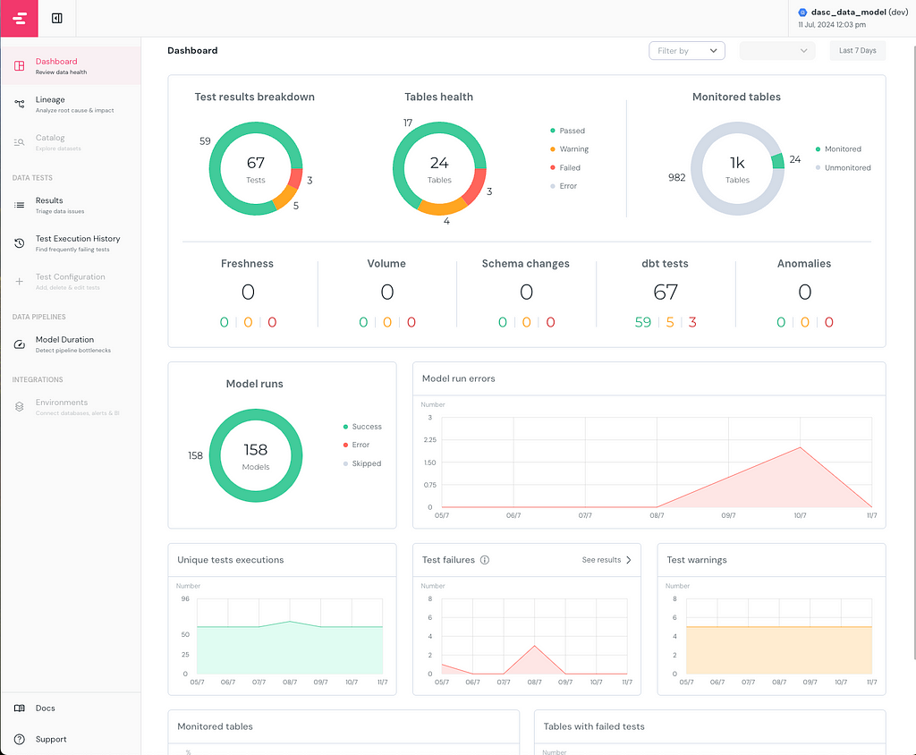
On the left lane of the dashboard, you can see the different pages, the Dashboard page gives a comprehensive overview of the dbt project’s performance and status. Catalog and Test Configuration pages are only available in Elementary Cloud but these configurations can also be implemented manually in the OSS version, explained more in detail in part 2.

• How to read this report?

In this exemplary report, I intentionally created warnings and errors beforehand for this article. 67 Tests were running in total, where 3 of them failed and 5 of them gave a warning. I monitored 24 tables, and all tests configured and checked were here dbt tests, if freshness or volume tests of Elementary had been configured, they would show up in the second row of the first visual.

As you can see in the Model runs visual, I have run 158 models without any errors or skipping. In the previous days, there were an increasing number of errors while running the models. I can easily see the errors that started occurring on 09/7 and troubleshoot them accordingly.

You can host this dashboard on your production and send it to your communication/alerting channel. Below is an example from an Argo workflow, but you can also check here for different methods that fit your setup/where you want to host it in your production.

- name: generate-elementary-report
    container:
      image: "{{inputs.parameters.elementary_image}}" ##pre-defined elemantary image in configmap.yaml
      command: ["edr"] ##run command for elemantary report
      args: ["report", "--profile-target={{inputs.parameters.target}}"]
      workingDir: workdir ##working directory
    inputs:
      parameters:
        - name: target
        - name: elementary_image
        - name: bucket
      artifacts:
        - name: source
          path: workdir ##working directory
    outputs:
      artifacts:
        - name: state
          path: /workdir/edr_target
          gcs:
            bucket: "{{inputs.parameters.bucket}}" ##here is the bucket that you would like to host your dashboard output
            key: path_to_key
          archive:
            none: {}

By using the template above in our Argo workflows, we would create the Elementary HTML report and save it in the defined bucket. We can later take this report from your bucket and send it with your alerts.

Now we know how we set up our report and hopefully know the basics of Elementary, next, we will check different types of tests and which test would suit the best in which scenario. Just jump into Part 2.

If that was enough for you already, thanks a lot for reading!

References in This Article

• Elementary Data Documentation. (n.d.). Elementary Data Documentation. Retrieved September 5, 2024, from https://docs.elementary-data.com
• dbt Labs. (n.d.). dbt Documentation. Retrieved September 5, 2024, from https://docs.getdbt.com
• Elementary Data. (n.d.). GitHub Repository. Retrieved September 5, 2024, from https://github.com/elementary-data
• dbt Labs. (2024). Upgrading to dbt v1.8. Retrieved September 5, 2024, from https://docs.getdbt.com/docs/dbt-versions/core-upgrade/upgrading-to-v1.8#deprecated-functionality
• Elementary Data. (n.d.). Elementary in Production. Retrieved September 5, 2024, from https://docs.elementary-data.com/oss/deployment-and-configuration/elementary-in-production#ways-to-run-elementary-in-production

---

Open-Source Data Observability with Elementary — From Zero to Hero (Part 1) was originally published in Towards Data Science on Medium, where people are continuing the conversation by highlighting and responding to this story.

Hands-on guide with side-by-side examples in Pandas

This article is not about comparing Polars with Pandas or highlighting their differences. It’s a story about how adding a new tool can be beneficial not only for data science professionals but also for others who work with data. I like Polars because it is multithreaded, providing strong performance out-of-the-box, and it supports Lazy evaluation with query optimization capabilities. This tool will undoubtedly enhance your data skills and open up new opportunities.

Although Polars and Pandas are different libraries, they share similarities in their APIs. Drawing parallels between them can make it easier for those familiar with the Pandas API to start using Polars. Even if you’re not familiar with Pandas and want to start learning Polars, it will still be incredibly useful and rewarding.

We will look at the most common actions that, in my experience, are most often used for data analysis. To illustrate the process of using Polars, I will consider an abstract task with reproducible data, so you can follow all the steps on your computer.

Imagine that we have data from three online stores, where we register user actions, such as viewing and purchasing. Let’s assume that at any given time, only one action of each type can occur for each online store, and in case of a transaction error, our data might be missing the product identifier or its quantity. Additionally, for our task, we’ll need a product catalog with prices for each item.

Let’s formulate the main task: to calculate a summary table with the total purchase for each online store.

I will break down this task into the following steps:

1. Data preparation and DataFrame creation.
2. Summary statistics of the DataFrame.
3. Retrieving the first five records.
4. Renaming columns.
5. Changing column types.
6. Filling missing values.
7. Removing missing values.
8. Removing duplicate records.
9. Filtering data.
10. Selecting the required columns.
11. Grouping data.
12. Merging data with another DataFrame.
13. Calculating a new column.
14. Creating a Pivot table.

Let’s get started!

Data Preparation and DataFrame Creation

We have the following data:

• OnlineStore — indicates the store.
• product — stores the product ID.
• Action type — the type of action (either a view or a purchase).
• quantity — the amount of the purchased or viewed product.
• Action_time — the timestamp for the action.

Requirements:

polars==1.6.0
pandas==2.0.0

from dataclasses import dataclass
from datetime import datetime, timedelta
from random import choice, gauss, randrange, seed
from typing import Any, Dict

import polars as pl
import pandas as pd

seed(42)

base_time= datetime(2024, 8, 31, 0, 0, 0, 0)

user_actions_data = [
    {
        "OnlineStore": choice(["Shop1", "Shop2", "Shop3"]),
        "product": choice(["0001", "0002", "0003"]),
        "quantity": choice([1.0, 2.0, 3.0]),
        "Action type": ("purchase" if gauss() > 0.6 else "view"),
        "Action_time": base_time - timedelta(minutes=randrange(1_000_000)),
    }
    for x in range(1_000_000)
]

corrupted_data = [
    {
        "OnlineStore": choice(["Shop1", "Shop2", "Shop3"]),
        "product": choice(["0001", None]),
        "quantity": choice([1.0, None]),
        "Action type": ("purchase" if gauss() > 0.6 else "view"),
        "Action_time": base_time - timedelta(minutes=randrange(1_000)),
    }
    for x in range(1_000)
]

For product catalog, which in our case include only product_id and its price (price).

product_catalog_data = {"product_id": ["0001", "0002", "0003"], "price": [100, 25, 80]}

The data is ready. Now let’s create DataFrames using these data with Pandas and Polars:

# Pandas
user_actions_pd_df = pd.DataFrame(user_actions_data)
corrupted_pd_df = pd.DataFrame(corrupted_data)
product_catalog_pd_df = pd.DataFrame(product_catalog_data)

# Polars
user_actions_pl_df = pl.DataFrame(user_actions_data)
corrupted_pl_df = pl.DataFrame(corrupted_data)
product_catalog_pl_df = pl.DataFrame(product_catalog_data)

Since we have user_actions_df and corrupted_df, let’s concatenate them into a single DataFrame.

# Pandas
user_actions_pd_df = pd.concat([user_actions_pd_df, corrupted_pd_df])

# Polars
user_actions_pl_df = pl.concat([user_actions_pl_df, corrupted_pl_df])

In this way, we have easily created DataFrames for further work.

Of course, each method has its own parameters, so it’s best to have the documentation handy to avoid confusion and use them appropriately.

Summary Statistics of the DataFrame

After loading or preparing data, it’s useful to quickly explore the resulting dataset. For summary statistics, the method name remains the same, but the results may differ:

# Pandas
user_actions_pd_df.describe(include='all')

       OnlineStore  product      quantity Action type          Action_time
count      1001000  1000492  1.000510e+06     1001000              1001000
unique           3        3           NaN           2               632335
top          Shop3     0001           NaN        view  2024-08-30 22:02:00
freq        333931   333963           NaN      726623                    9
first          NaN      NaN           NaN         NaN  2022-10-06 13:23:00
last           NaN      NaN           NaN         NaN  2024-08-30 23:58:00
mean           NaN      NaN  1.998925e+00         NaN                  NaN
std            NaN      NaN  8.164457e-01         NaN                  NaN
min            NaN      NaN  1.000000e+00         NaN                  NaN
25%            NaN      NaN  1.000000e+00         NaN                  NaN
50%            NaN      NaN  2.000000e+00         NaN                  NaN
75%            NaN      NaN  3.000000e+00         NaN                  NaN
max            NaN      NaN  3.000000e+00         NaN                  NaN

# Polars
user_actions_pl_df.describe()

┌────────────┬─────────────┬─────────┬───────────┬─────────────┬────────────────────────────┐
│ statistic  ┆ OnlineStore ┆ product ┆ quantity  ┆ Action type ┆ Action_time                │
│ ---        ┆ ---         ┆ ---     ┆ ---       ┆ ---         ┆ ---                        │
│ str        ┆ str         ┆ str     ┆ f64       ┆ str         ┆ str                        │
╞════════════╪═════════════╪═════════╪═══════════╪═════════════╪════════════════════════════╡
│ count      ┆ 1001000     ┆ 1000492 ┆ 1.00051e6 ┆ 1001000     ┆ 1001000                    │
│ null_count ┆ 0           ┆ 508     ┆ 490.0     ┆ 0           ┆ 0                          │
│ mean       ┆ null        ┆ null    ┆ 1.998925  ┆ null        ┆ 2023-09-19 03:24:30.981698 │
│ std        ┆ null        ┆ null    ┆ 0.816446  ┆ null        ┆ null                       │
│ min        ┆ Shop1       ┆ 1       ┆ 1.0       ┆ purchase    ┆ 2022-10-06 13:23:00        │
│ 25%        ┆ null        ┆ null    ┆ 1.0       ┆ null        ┆ 2023-03-29 03:09:00        │
│ 50%        ┆ null        ┆ null    ┆ 2.0       ┆ null        ┆ 2023-09-19 06:49:00        │
│ 75%        ┆ null        ┆ null    ┆ 3.0       ┆ null        ┆ 2024-03-11 03:01:00        │
│ max        ┆ Shop3       ┆ 3       ┆ 3.0       ┆ view        ┆ 2024-08-30 23:58:00        │
└────────────┴─────────────┴─────────┴───────────┴─────────────┴────────────────────────────┘

As you can notice, Pandas calculates statistics differently for various data types and provides unique values for all columns. Polars, on the other hand, calculates the null_count value.

Additionally, in the Polars documentation, it is stated:

We do not guarantee the output of describe to be stable. It will show statistics that we deem informative, and may be updated in the future. Using describe programmatically (versus interactive exploration) is not recommended for this reason.

Retrieving the First Five Records

When encountering data for the first time, we always want to explore it. Beyond obtaining summary statistics, it’s also important to see the actual records it contains. To do this, we often look at the first five records as a sample.

# Pandas
user_actions_pd_df.head()

  OnlineStore product  quantity Action type         Action_time
0       Shop3    0001       1.0        view 2024-05-21 09:24:00
1       Shop3    0001       3.0        view 2023-03-10 15:54:00
2       Shop3    0001       3.0        view 2024-03-24 19:02:00
3       Shop1    0003       3.0        view 2024-08-11 16:16:00
4       Shop3    0001       3.0        view 2024-03-23 11:32:00

# Polars
user_actions_pl_df.head()

┌─────────────┬─────────┬──────────┬─────────────┬─────────────────────┐
│ OnlineStore ┆ product ┆ quantity ┆ Action type ┆ Action_time         │
│ ---         ┆ ---     ┆ ---      ┆ ---         ┆ ---                 │
│ str         ┆ str     ┆ f64      ┆ str         ┆ datetime[μs]        │
╞═════════════╪═════════╪══════════╪═════════════╪═════════════════════╡
│ Shop3       ┆ 0001    ┆ 1.0      ┆ view        ┆ 2024-05-21 09:24:00 │
│ Shop3       ┆ 0001    ┆ 3.0      ┆ view        ┆ 2023-03-10 15:54:00 │
│ Shop3       ┆ 0001    ┆ 3.0      ┆ view        ┆ 2024-03-24 19:02:00 │
│ Shop1       ┆ 0003    ┆ 3.0      ┆ view        ┆ 2024-08-11 16:16:00 │
│ Shop3       ┆ 0001    ┆ 3.0      ┆ view        ┆ 2024-03-23 11:32:00 │
└─────────────┴─────────┴──────────┴─────────────┴─────────────────────┘

Polars has a useful glimpse() function that provides a dense preview of the DataFrame. It not only returns the first 10 records (or any number you specify using the max_items_per_column parameter) but also shows data types and record counts.

# Polars
user_actions_pl_df.glimpse()

Rows: 1001000
Columns: 5
$ OnlineStore          <str> 'Shop3', 'Shop3', 'Shop3', 'Shop1', 'Shop3', 'Shop2', 'Shop1', 'Shop2', 'Shop1', 'Shop2'
$ product              <str> '0001', '0001', '0001', '0003', '0001', '0003', '0001', '0001', '0002', '0003'
$ quantity             <f64> 1.0, 3.0, 3.0, 3.0, 3.0, 2.0, 3.0, 1.0, 2.0, 1.0
$ Action type          <str> 'view', 'view', 'view', 'view', 'view', 'view', 'view', 'view', 'view', 'view'
$ Action_time <datetime[μs]> 2024-05-21 09:24:00, 2023-03-10 15:54:00, 2024-03-24 19:02:00, 2024-08-11 16:16:00, 2024-03-23 11:32:00, 2023-01-19 14:11:00, 2024-03-27 05:08:00, 2023-11-28 08:18:00, 2023-03-18 15:01:00, 2022-10-29 09:44:00

Renaming Columns

After exploring the data, it is often necessary to edit it for further use. If the column names are not satisfactory or if your company has its own naming conventions, you can easily rename them.

# Pandas
user_actions_pd_df = user_actions_pd_df.rename(
    columns={
        "OnlineStore": "online_store",
        "product": "product_id",
        "Action type": "action_type",
        "Action_time": "action_dt",
    }
)

# user_actions_pd_df.columns
Index(['online_store', 'product_id', 'quantity', 'action_type', 'action_dt'], dtype='object')

# Polars
user_actions_pl_df = user_actions_pl_df.rename(
    {
        "OnlineStore": "online_store",
        "product": "product_id",
        "Action type": "action_type",
        "Action_time": "action_dt",
    }
)

# user_actions_pl_df.columns
['online_store', 'product_id', 'quantity', 'action_type', 'action_dt']

Changing Column Types

When working with data, optimizing their processing is often a priority, and data types are no exception. Choosing the right type not only unlocks available functions but also saves memory. In our example, I will change the column type of quantity from float to int. In Pandas, you would use the astype() method, while in Polars, you use the cast() method.

# Pandas
user_actions_pd_df = user_actions_pd_df.astype({"quantity": "Int64"})

Int64Index: 1001000 entries, 0 to 999
Data columns (total 5 columns):
 #   Column        Non-Null Count    Dtype         
---  ------        --------------    -----         
 0   online_store  1001000 non-null  object        
 1   product_id    1000492 non-null  object        
 2   quantity      1000510 non-null  Int64         
 3   action_type   1001000 non-null  object        
 4   action_dt     1001000 non-null  datetime64[ns]
dtypes: Int64(1), datetime64[ns](1), object(3)
memory usage: 46.8+ MB

# Polars
user_actions_pl_df = user_actions_pl_df.cast({"quantity": pl.Int32})

Rows: 1001000
Columns: 5
$ online_store          <str> 
$ product_id            <str> 
$ quantity              <i32> 
$ action_type           <str> 
$ action_dt    <datetime[μs]> 

Polars has a special method estimated_size() that returns an estimate of the total (heap) allocated size of the DataFrame. For example:

user_actions_pl_df.estimated_size("mb")
# Result: 24.91054630279541

Although the method names for changing types differ, SQL enthusiasts will appreciate the ease of transition.

Filling Missing Values

In real projects, data is rarely perfect, and we often discuss with managers, analysts, and other systems how to interpret data behavior. During data preparation, I specifically generated corrupted_data to introduce some chaos into the data. Handling missing values could easily be the subject of an entire book.

There are several strategies for filling in missing values, and the choice of method depends on the task: sometimes filling missing values with zeros is sufficient, while other times the mean value may be used. In Polars, the fill_null() method can be applied both to the DataFrame and to specific columns. To add a new column or replace values in an existing one, the with_columns() method is also used.

In our example, I will fill missing values in the quantity column with 0:

# Pandas
user_actions_pd_df["quantity"].fillna(0, inplace=True)

Data columns (total 5 columns):
 #   Column        Non-Null Count    Dtype         
---  ------        --------------    -----         
 0   online_store  1001000 non-null  object        
 1   product_id    1000492 non-null  object        
 2   quantity      1001000 non-null  Int64         
 3   action_type   1001000 non-null  object        
 4   action_dt     1001000 non-null  datetime64[ns]
dtypes: Int64(1), datetime64[ns](1), object(3)

# Polars
user_actions_pl_df = user_actions_pl_df.with_columns(pl.col("quantity").fill_null(0))

┌────────────┬──────────────┬────────────┬──────────┬─────────────┬────────────────────────────┐
│ statistic  ┆ online_store ┆ product_id ┆ quantity ┆ action_type ┆ action_dt                  │
│ ---        ┆ ---          ┆ ---        ┆ ---      ┆ ---         ┆ ---                        │
│ str        ┆ str          ┆ str        ┆ f64      ┆ str         ┆ str                        │
╞════════════╪══════════════╪════════════╪══════════╪═════════════╪════════════════════════════╡
│ count      ┆ 1001000      ┆ 1000492    ┆ 1.001e6  ┆ 1001000     ┆ 1001000                    │
│ null_count ┆ 0            ┆ 508        ┆ 0.0      ┆ 0           ┆ 0                          │
└────────────┴──────────────┴────────────┴──────────┴─────────────┴────────────────────────────┘

In Polars, you can use various strategies for filling missing values in the data, such as: {None, ‘forward’, ‘backward’, ‘min’, ‘max’, ‘mean’, ‘zero’, ‘one’}. The names of these strategies are self-explanatory, so we won’t delve into their details.

It’s also worth noting that for filling NaN values in floating-point columns, you should use the fill_nan() method, which does not involve strategies.

Removing Missing Values

Not all missing values can be filled, so those that cannot be correctly filled and used in further calculations are best removed. In our case, this applies to the product_id column, as we cannot compute the final result without this identifier.

To remove rows with missing values in Pandas and Polars, use the following methods:

# Pandas
user_actions_pd_df.dropna(subset=["product_id"], inplace=True)

Int64Index: 1000492 entries, 0 to 999
Data columns (total 5 columns):
 #   Column        Non-Null Count    Dtype         
---  ------        --------------    -----         
 0   online_store  1000492 non-null  object        
 1   product_id    1000492 non-null  object        
 2   quantity      1000492 non-null  Int64         
 3   action_type   1000492 non-null  object        
 4   action_dt     1000492 non-null  datetime64[ns]
dtypes: Int64(1), datetime64[ns](1), object(3)

# Polars
user_actions_pl_df = user_actions_pl_df.drop_nulls(subset=["product_id"])

┌────────────┬──────────────┬────────────┬────────────┬─────────────┬────────────────────────────┐
│ statistic  ┆ online_store ┆ product_id ┆ quantity   ┆ action_type ┆ action_dt                  │
│ ---        ┆ ---          ┆ ---        ┆ ---        ┆ ---         ┆ ---                        │
│ str        ┆ str          ┆ str        ┆ f64        ┆ str         ┆ str                        │
╞════════════╪══════════════╪════════════╪════════════╪═════════════╪════════════════════════════╡
│ count      ┆ 1000492      ┆ 1000492    ┆ 1.000492e6 ┆ 1000492     ┆ 1000492                    │
│ null_count ┆ 0            ┆ 0          ┆ 0.0        ┆ 0           ┆ 0                          │
└────────────┴──────────────┴────────────┴────────────┴─────────────┴────────────────────────────┘

It’s also worth noting that to remove NaN values in floating-point columns, you should use the drop_nans() method.

Removing Duplicate Records

The simplest case of duplicate records occurs when all values of one record are identical to another. In our case, duplicates might arise if the same action is recorded multiple times for the same action type in the same online store at a single point in time. I will keep only the most recent value in case duplicates are found.

To remove duplicate records in Pandas, use the drop_duplicates() method, and in Polars, the unique() method.

# Pandas
user_actions_pd_df.drop_duplicates(
    subset=["online_store", "action_type", "action_dt"],
    keep="last",
    inplace=True,
)

Data columns (total 5 columns):
 #   Column        Non-Null Count   Dtype         
---  ------        --------------   -----         
 0   online_store  907246 non-null  object        
 1   product_id    907246 non-null  object        
 2   quantity      907246 non-null  Int64         
 3   action_type   907246 non-null  object        
 4   action_dt     907246 non-null  datetime64[ns]
dtypes: Int64(1), datetime64[ns](1), object(3)

# Polars
user_actions_pl_df = user_actions_pl_df.unique(
    subset=["online_store", "action_type", "action_dt"],
    keep="last",
)

┌────────────┬──────────────┬────────────┬──────────┬─────────────┬────────────────────────────┐
│ statistic  ┆ online_store ┆ product_id ┆ quantity ┆ action_type ┆ action_dt                  │
│ ---        ┆ ---          ┆ ---        ┆ ---      ┆ ---         ┆ ---                        │
│ str        ┆ str          ┆ str        ┆ f64      ┆ str         ┆ str                        │
╞════════════╪══════════════╪════════════╪══════════╪═════════════╪════════════════════════════╡
│ count      ┆ 907246       ┆ 907246     ┆ 907246.0 ┆ 907246      ┆ 907246                     │
│ null_count ┆ 0            ┆ 0          ┆ 0.0      ┆ 0           ┆ 0                          │
└────────────┴──────────────┴────────────┴──────────┴─────────────┴────────────────────────────┘

Filtering Data

After the data cleaning phase, we need to filter the relevant data for future calculations. In Polars, this is done using the method with a quite descriptive name, filter().

Rows where the filter does not evaluate to True are discarded, including nulls.

# Pandas
user_actions_pd_df = user_actions_pd_df.loc[
    user_actions_pd_df["action_type"] == "purchase"
]

Int64Index: 262237 entries, 11 to 995
Data columns (total 5 columns):
 #   Column        Non-Null Count   Dtype         
---  ------        --------------   -----         
 0   online_store  262237 non-null  object        
 1   product_id    262237 non-null  object        
 2   quantity      262237 non-null  Int64         
 3   action_type   262237 non-null  object        
 4   action_dt     262237 non-null  datetime64[ns]
dtypes: Int64(1), datetime64[ns](1), object(3)

# Polars
user_actions_pl_df = user_actions_pl_df.filter(
    pl.col("action_type") == "purchase"
)

┌────────────┬──────────────┬────────────┬──────────┬─────────────┬────────────────────────────┐
│ statistic  ┆ online_store ┆ product_id ┆ quantity ┆ action_type ┆ action_dt                  │
│ ---        ┆ ---          ┆ ---        ┆ ---      ┆ ---         ┆ ---                        │
│ str        ┆ str          ┆ str        ┆ f64      ┆ str         ┆ str                        │
╞════════════╪══════════════╪════════════╪══════════╪═════════════╪════════════════════════════╡
│ count      ┆ 262237       ┆ 262237     ┆ 262237.0 ┆ 262237      ┆ 262237                     │
│ null_count ┆ 0            ┆ 0          ┆ 0.0      ┆ 0           ┆ 0                          │
└────────────┴──────────────┴────────────┴──────────┴─────────────┴────────────────────────────┘

Selecting Required Columns

After filtering the data, you may need to retain only the columns relevant for further analysis. In Polars, this is achieved using the select() method.

# Pandas
user_actions_pd_df = user_actions_pd_df[
    ["online_store", "action_type", "product_id", "quantity"]
]

# Polars
user_actions_pl_df = user_actions_pl_df.select(
    "online_store", "action_type", "product_id", "quantity"
)

Grouping Data

After preparing the data, we can aggregate it to get the sum of quantity for each online store and product. I will also retain action_type for further steps. We use the group_by() method in Polars, which is similar to the groupby() method in Pandas.

# Pandas
user_actions_pd_df = (
    user_actions_pd_df.groupby(["online_store", "product_id", "action_type"])
    .agg({"quantity": "sum"})
    .reset_index()
)

  online_store product_id action_type  quantity
0        Shop1       0001    purchase     57772
1        Shop1       0002    purchase     58015
2        Shop1       0003    purchase     58242
3        Shop2       0001    purchase     58256
4        Shop2       0002    purchase     58648
5        Shop2       0003    purchase     58458
6        Shop3       0001    purchase     57891
7        Shop3       0002    purchase     58326
8        Shop3       0003    purchase     59107

# Polars
user_actions_pl_df = (
    user_actions_pl_df.group_by(["online_store", "product_id", "action_type"])
    .agg(pl.col("quantity").sum())
)

┌──────────────┬────────────┬─────────────┬──────────┐
│ online_store ┆ product_id ┆ action_type ┆ quantity │
│ ---          ┆ ---        ┆ ---         ┆ ---      │
│ str          ┆ str        ┆ str         ┆ i32      │
╞══════════════╪════════════╪═════════════╪══════════╡
│ Shop1        ┆ 0001       ┆ purchase    ┆ 57772    │
│ Shop1        ┆ 0002       ┆ purchase    ┆ 58015    │
│ Shop1        ┆ 0003       ┆ purchase    ┆ 58242    │
│ Shop2        ┆ 0001       ┆ purchase    ┆ 58256    │
│ Shop2        ┆ 0002       ┆ purchase    ┆ 58648    │
│ Shop2        ┆ 0003       ┆ purchase    ┆ 58458    │
│ Shop3        ┆ 0001       ┆ purchase    ┆ 57891    │
│ Shop3        ┆ 0002       ┆ purchase    ┆ 58326    │
│ Shop3        ┆ 0003       ┆ purchase    ┆ 59107    │
└──────────────┴────────────┴─────────────┴──────────┘

Joining Data with Another DataFrame

To calculate the total purchases, we need to join our data with the price catalog. In Pandas, we have two methods for this, join() and merge(), which differ in their specifics and functionality. In Polars, we use only the join() method.

# Pandas
user_actions_pd_df = user_actions_pd_df.merge(product_catalog_pd_df, on='product_id')

  online_store product_id action_type  quantity  price
0        Shop1       0001    purchase     57772    100
3        Shop1       0002    purchase     58015     25
6        Shop1       0003    purchase     58242     80
1        Shop2       0001    purchase     58256    100
4        Shop2       0002    purchase     58648     25
7        Shop2       0003    purchase     58458     80
2        Shop3       0001    purchase     57891    100
5        Shop3       0002    purchase     58326     25
8        Shop3       0003    purchase     59107     80

# Polars
user_actions_pl_df = user_actions_pl_df.join(product_catalog_pl_df, on='product_id')

┌──────────────┬────────────┬─────────────┬──────────┬───────┐
│ online_store ┆ product_id ┆ action_type ┆ quantity ┆ price │
│ ---          ┆ ---        ┆ ---         ┆ ---      ┆ ---   │
│ str          ┆ str        ┆ str         ┆ i32      ┆ i64   │
╞══════════════╪════════════╪═════════════╪══════════╪═══════╡
│ Shop1        ┆ 0001       ┆ purchase    ┆ 57772    ┆ 100   │
│ Shop1        ┆ 0002       ┆ purchase    ┆ 58015    ┆ 25    │
│ Shop1        ┆ 0003       ┆ purchase    ┆ 58242    ┆ 80    │
│ Shop2        ┆ 0001       ┆ purchase    ┆ 58256    ┆ 100   │
│ Shop2        ┆ 0002       ┆ purchase    ┆ 58648    ┆ 25    │
│ Shop2        ┆ 0003       ┆ purchase    ┆ 58458    ┆ 80    │
│ Shop3        ┆ 0001       ┆ purchase    ┆ 57891    ┆ 100   │
│ Shop3        ┆ 0002       ┆ purchase    ┆ 58326    ┆ 25    │
│ Shop3        ┆ 0003       ┆ purchase    ┆ 59107    ┆ 80    │
└──────────────┴────────────┴─────────────┴──────────┴───────┘

In Polars, the how parameter supports the following values: {‘inner’, ‘left’, ‘right’, ‘full’, ‘semi’, ‘anti’, ‘cross’} .

Calculating a New Column

To calculate a new column or modify an existing column, Polars uses the with_columns() method. To set an alias for a column, you can use alias().

# Pandas
user_actions_pd_df["total"] = (
    user_actions_pd_df["price"] * user_actions_pd_df["quantity"]
)
user_actions_pd_df = user_actions_pd_df[
    ["online_store", "action_type", "total"]
]

# Polars
user_actions_pl_df = user_actions_pl_df.with_columns(
    (pl.col("price") * pl.col("quantity")).alias("total")
)
user_actions_pl_df = user_actions_pl_df.select(
    "online_store", "action_type", "total"
)

Alternatively, you can calculate a new column directly within the select() method:

# Polars
user_actions_pl_df = user_actions_pl_df.select(
    "online_store",
    "action_type",
    (pl.col("price") * pl.col("quantity")).alias("total"),
)

Creating a Pivot Table

Our final step is to create a pivot table. We have already calculated the total sales for each product, and now we will easily calculate the total sales for each online store. In Pandas, we use the pivot_table() method, which allows for the application of aggregate functions. In Polars, we use the pivot() method to create the pivot table.

# Pandas
result_pd = user_actions_pd_df.pivot_table(
    columns="online_store",
    index="action_type",
    values="total",
    aggfunc="sum",
)

online_store     Shop1     Shop2     Shop3
action_type                               
purchase      11886935  11968440  11975810

# Polars
result_pl = user_actions_pl_df.pivot(
    columns="online_store",
    index="action_type",
    values="total",
    aggregate_function="sum",
)

┌─────────────┬──────────┬──────────┬──────────┐
│ action_type ┆ Shop1    ┆ Shop2    ┆ Shop3    │
│ ---         ┆ ---      ┆ ---      ┆ ---      │
│ str         ┆ i64      ┆ i64      ┆ i64      │
╞═════════════╪══════════╪══════════╪══════════╡
│ purchase    ┆ 11886935 ┆ 11968440 ┆ 11975810 │
└─────────────┴──────────┴──────────┴──────────┘

DeprecationWarning: The argument columns for pl.DataFrame.pivot` is deprecated. It has been renamed to on.

Here we are, concluding our little journey. As we can see, the results for both Pandas and Polars match. Everyone who made it to this point is great and incredibly hardworking — you will succeed!

Summary

In this article, we explored Polars using practical examples and comparisons with Pandas. I demonstrated how to handle data preparation, descriptive statistics, missing values, duplicates, filtering, column selection, grouping, merging, and pivot tables. By showcasing these tasks with both Pandas and Polars, I highlighted the ease of using Polars and transitioning to it from Pandas. This guide serves as a practical introduction to leveraging Polars for efficient data analysis.

Recommended read:

• Improving Code Quality During Data Transformation with Polars

Thanks for Reading!

If you enjoyed this article and want to support my work, the best way is to follow me on Medium. Let’s connect on LinkedIn if you’re also interested in working with data like I am. Your claps are greatly appreciated — they help me know how useful this post was for you.

---

Practical Introduction to Polars was originally published in Towards Data Science on Medium, where people are continuing the conversation by highlighting and responding to this story.