Dimensionality reduction through Principal Component Analysis (PCA).
Originally appeared here:
Principal Component Analysis — Hands-On Tutorial
Go Here to Read this Fast! Principal Component Analysis — Hands-On Tutorial

Dimensionality reduction through Principal Component Analysis (PCA).
Originally appeared here:
Principal Component Analysis — Hands-On Tutorial
Go Here to Read this Fast! Principal Component Analysis — Hands-On Tutorial

Markov Decision Processes are foundational to sequential decision-making problems and serve as the building block for reinforcement learning. They model the dynamic interaction between an agent having to make a series of actions and their environment. Due to their wide applicability in fields such as robotics, finance, operations research and AI, MDPs have been extensively studied in both theoretical and practical contexts.
Yet, much of the existing MDP literature focuses on the idealized scenarios where model parameters — such as transition probabilities and reward functions — are assumed to be known with certainty. In practice, applying popular methods such as Policy Iteration and Value Iteration require precise estimates of these parameters, often obtained from real-world data. This reliance on data introduces significant challenges: the estimation process is inherently noisy and sensitive to limitations such as data scarcity, measurement errors and variability in the observed environment. Consequently, the performance of standard MDP methods can degrade substantially when applied to problems with uncertain or incomplete data.
In this article, we build on the Robust Optimization (RO) literature to propose a generic framework to address these issues. We provide a Robust Linear Programming (RLP) formulation of MDPs that is capable of handling various sources of uncertainty and adversarial perturbations.
Let’s start by giving a formal definition of MDPs:
A Markov Decision Process is a 5-tuple (S, A, R, P, γ) such that:
We then define the policy, i.e. what dictates the agent’s behavior in an MDP:
A policy π is a probability measure over the action space defined as: π(a|s) is the probability of taking action a when the agent is in state s.
We finally introduce the value function, i.e. the agent’s objective in an MDP:
The value function of a policy π is the expected discounted reward under this policy, when starting at a given state s:

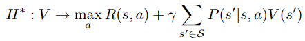
In particular, the value function of the optimal policy π* satisfies the Bellman optimality equation:

Which yields the deterministic optimal policy:

Given the above definitions, we can start by noticing that any value function V that satisfies

is an upper bound on the optimal value function. To see it, we can start by noticing that such value function also satisfies:

We recognize the value iteration operator applied to V:
i.e.

Also noticing that the H*operator is increasing, we can apply it iteratively to have:

where we used the property of V* being the fixed point of H*.
Therefore, finding V* comes down to finding the tightest upper bound V that obeys the above equation, which yields the following formulation:
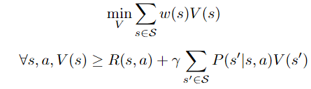
Here we added a weight term corresponding to the probability of starting in state s. We can see that the above problem is linear in V and can be rewritten as follows:
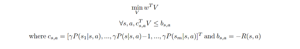
Further details can be found in [1] and [2].
Given the above linear program in standard form, the RO framework assumes an adversarial noise in the inputs (i.e. cost vector and constraints). To model this uncertainty, we define an uncertainty set:

In short, we want to find the minimum of all linear programs, i.e. for each occurrence in the uncertainty set. Naturally this yields a completely intractable model (potentially an infinite number of LPs) since we did not make any assumption on the form of U.
Before addressing these issues, we make the following assumptions — without loss of generality:
where: bar{c} is known as the nominal constraint vector (e.g. gotten from some estimation), z the uncertain factor and Q a fixed matrix intuitively corresponding to how the noise is applied to each coefficient of the constraint vector. Q can be used for instance to model correlation between the noise on difference components of c. See [3] for more details and proofs.
Note: we made a slight abuse of notation and dropped the (s, a) subscripts for readability — yet c, bar{c}, Q and z are all for a given state and action couple.
All this leads to the following formulation of the problem:

At this stage, we can make some assumptions on the form of U in order to further simplify the problem:
The optimization problem becomes:

which is equivalent to:

Finally, looking closer to the maximization problem in the constraint, we see that it has a closed form. Therefore the final problem can be written as (robust counterpart of a linear program with box uncertainty):

A few comments on the above formulation:
For more details, the interested reader can refer to [3].
Starting from the above formulation:

And finally, linearizing the absolute value in the constraints gives:

We notice that robustness translates into an additional safety term in the constraints — given the uncertainty on c (which mainly translates into uncertainty in the MDP’s transition probabilities).
As stated previously, considering uncertainty on the rewards as well can be easily done with a similar derivation. Coming back to the linear program in standard form, we add another noise term on the right hand side of the constraints:

After a similar reasoning as previously done, we have the all-in linear program:

Again similarly to before, additional robustness with regards to the reward function translates into another safety term in the constraints, which ultimately can yield a less optimal value function and policy but fills the constraints with margin. This tradeoff is controlled both by Q and the size of the uncertainty box d.
While this completes the derivation of the Robust MDP as a linear program, other robust MDP approaches have been developed in the literature, see for instance [4]. These approaches usually take a different route, for instance directly deriving a robust Policy Evaluation operator — which for instance has the advantage of having a better complexity as the LP approach. This proves particularly important when state and action spaces are large. Therefore why would we use such formulation?
[1] M.L. Puterman, Markov Decision Processes: Discrete Stochastic Dynamic Programming (1996), Wiley
[2] P. Pouppart, Sequential Decision Making and Reinforcement Learning (2013), University of Waterloo
[3] D. Bertsimas, D. Den Hertog, Robust and Adaptive Optimization (2022), Dynamic Ideas
[4] W. Wiesemann, D. Kuhn, B. Rustem, Robust Markov Decision Processes (2013), INFORMS
[5] K. Vu, P.-L. Poirion, L. Liberti, Random Projections for Linear Programming (2018), INFORMS
Uncertainty in Markov Decisions Processes: a Robust Linear Programming approach was originally published in Towards Data Science on Medium, where people are continuing the conversation by highlighting and responding to this story.
Originally appeared here:
Uncertainty in Markov Decisions Processes: a Robust Linear Programming approach


Receive clear and useful feedback. Ditch generic questions. More than 60 example questions for you to use.
Originally appeared here:
Asking for Feedback as a Data Scientist Individual Contributor
Go Here to Read this Fast! Asking for Feedback as a Data Scientist Individual Contributor
Transform your data into actionable insights with customer segmentation for improved engagement and profitability
Originally appeared here:
Unlocking Business Potential Through Effective Customer Segmentation
Go Here to Read this Fast! Unlocking Business Potential Through Effective Customer Segmentation
Learn about Maximum Likelihood Estimates via their application for next-word prediction
Originally appeared here:
Introduction to Maximum Likelihood Estimates
Go Here to Read this Fast! Introduction to Maximum Likelihood Estimates


Have you ever wished your deep-learning model could run faster?
The GPU is expensive. The dataset is enormous, and the training session seems endless; you have a million experiments to run and a deadline to hit — all these are good reasons to expect a particular form of training acceleration.
But which one to choose?
There are already good references on performance tuning for model training from PyTorch, HuggingFace, and Nvidia, including asynchronous data loading, buffer checkpointing, distributed data parallelization, and automatic mixed precision.
In this article, I’ll introduce the automatic mixed precision technique. I’ll start with a brief introduction to Nvidia’s tensor core design, then the groundbreaking work “Mixed Precision Training” paper published in ICLR 2018, and lastly, proceed to a simple example of training a ResNet50 on FashionMNIST and how to speed up the training by 2X while loading 2X a batch size, with only three extra lines of code.
First, let’s recap some of the fundamentals of the GPU design. One of Nvidia GPUS’s most popular commercial products is the Volta family, e.g., V100 GPUs, based on the GV100 GPU design. So, we’ll base our discussions around the GV100 architecture below.
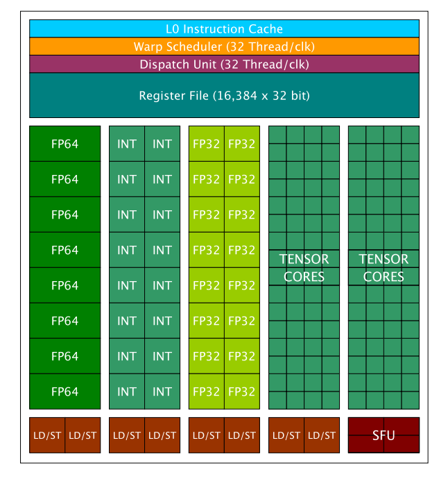
For GV100, the Streaming Multiprocessor (SM) is the core design for computation. Each GPU contains 6 GPU Processing Clusters (GPCs) and S84 SMs (or 80 SMs for V100). The overall design looks like the one below.

For each SM, it contains two types of cores: CUDA cores and Tensor cores. CUDA cores were Nvidia’s original design introduced in 2006, which was an essential part of the CUDA platform. The CUDA cores can be divided into three types: FP64 core/unit, FP32 core/unit, and Int32 core/unit. Each GV100 SM contains 32 FP64 cores, 64 FP32 cores, and 64 Int32 cores. Tensor cores were introduced in the Volta/Turing (2017) series GPUs to separate from the previous Pascal (2016) series. Each SM on a GV100 contains 8 Tensor cores. A full list of details is given here for V100 GPUs. A detailed look at the SM design is below.
Why Tensor cores? Nvidia Tensor cores are dedicated to performing general matrix multiplication (GEMM) and half-precision matrix multiplication and accumulation (HMMA) operations. In short, GEMM performs matrix operations in the format of A*B + C, and HMMA converts the operation into the half-precision format. A detailed discussion can be found here. Since deep learning involves MMA heavily, the Tensor cores are essential in today’s model training and speed-up.

Of course, when switching to mixed precision training, always check the specification of the GPU you’re using. Only the latest GPU series support Tensor cores, and mixed precision training can only be used on these machines.
Now, let’s take a closer look at FP32 and FP16 formats. The FP32 and FP16 are IEEE formats that represent floating numbers using 32-bit binary storage and 16-bit binary storage. Both formats comprise three parts: a) a sign bit, b) exponent bits, and c) mantissa bits. The FP32 and FP16 differ in the number of bits allocated to exponent and mantissa, which result in different value ranges and precisions.

How do you convert FP16 and FP32 to real values? According to IEEE-754 standards, the decimal value for FP32 = (-1)^(sign) × 2^(decimal exponent —127 ) × (implicit leading 1 + decimal mantissa), where 127 is the biased exponent value. For FP16, the formula becomes (-1)^(sign) × 2^(decimal exponent — 15) × (implicit leading 1 + decimal mantissa), where 15 is the corresponding biased exponent value. See further details of the biased exponent value here.
In this sense, the value range for FP32 is approximately [-2¹²⁷, 2¹²⁷] ~[-1.7*1e38, 1.7*1e38], and the value range for FP16 is approximately [-2¹⁵, 2¹⁵]=[-32768, 32768]. Note that the decimal exponent for FP32 is between 0 and 255, and we’re excluding the largest value 0xFF as it represents NAN. That’s why the largest decimal exponent is 254–127 = 127. A similar rule applies to FP16.
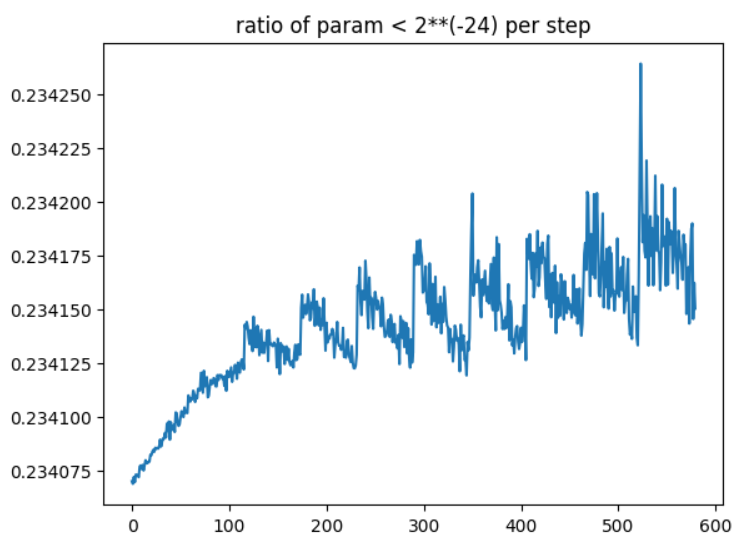
For the precision, note that both the exponent and mantissa contributes to the precision limits (which is also called denormalization, see detailed discussion here), so FP32 can represent precision up to 2^(-23)*2^(-126)=2^(-149), and FP16 can represent precision up to 2^(10)*2^(-14)=2^(-24).
The difference between FP32 and FP16 representations brings the key concerns of mixed precision training, as different layers/operations of deep learning models are either insensitive or sensitive to value ranges and precision and need to be addressed separately.
Now that we have learnt the hardware foundation for MMA, the concept of Tensor cores, and the key difference between FP32 and FP16, we can further discuss the details for mixed precision training.
The idea of mixed precision training was first proposed in the 2018 ICLR paper “Mixed Precision Training”, which converts deep learning models into half-precision floating point during training without losing model accuracy or modifying hyper-parameters. As mentioned above, since the key difference between FP32 and FP16 are the value ranges and precisions, the paper discussed in detail why the FP16 causes the gradients to vanish and how to fix the issue by loss scaling. Besides, the paper proposes tricks like using FP32 master weight copy and using FP32 for specific operations like reductions and vector dot-production accumulations.
Loss scaling. The paper gives an example of training a Multibox SSD detector network using FP32 precision, as shown below. Without any scaling, the exponent range of the FP16 gradients ≥ 2^(-24), and everything below would become zero, which is insufficient compared to FP32. However, with an experiment, scaling the gradients simply by 2³=8 times can bring the half-precision training accuracy back to match with FP32. In this sense, the authors argue that the extra few percent of gradients between [2^(-27), 2^(-24)] are still important in the training process, while the value below 2^(-27) is not important.
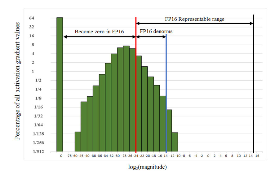
The way to address this scale difference is to apply loss scaling. According to the chain’s rule, scaling the loss will ensure the same amount scales all the gradients. The gradients need to be unscaled before the final weight update.
Nvidia first developed Automatic Mixed Precision Training as a PyTorch extension called APEX, which was then widely adopted by mainstream frameworks like PyTorch, TensorFlow, MXNet, etc. See Nvidia docs here. We’ll only introduce PyTorch’s automatic mixed precision library for simplicity: https://pytorch.org/docs/stable/amp.html.
The amp library can automatically handle most of the mixed precision training techniques, like the FP32 master weight copy. The users are mainly exposed to ops autocast and gradient/loss scaling.
Ops autocast. Although we mentioned that tensor cores could largely improve the performance of GEMM operations, certain operations are unsuitable for half-precision representations.
The amp library gives out a list of CUDA ops eligible for half precision. Most matrix multiplication, convolutions, and linear activations are fully covered by the amp.autocast, however, for reduction/sum, softmax, and loss calculations, the calculations are still performed in FP32 as they are more sensitive to data range and precision.
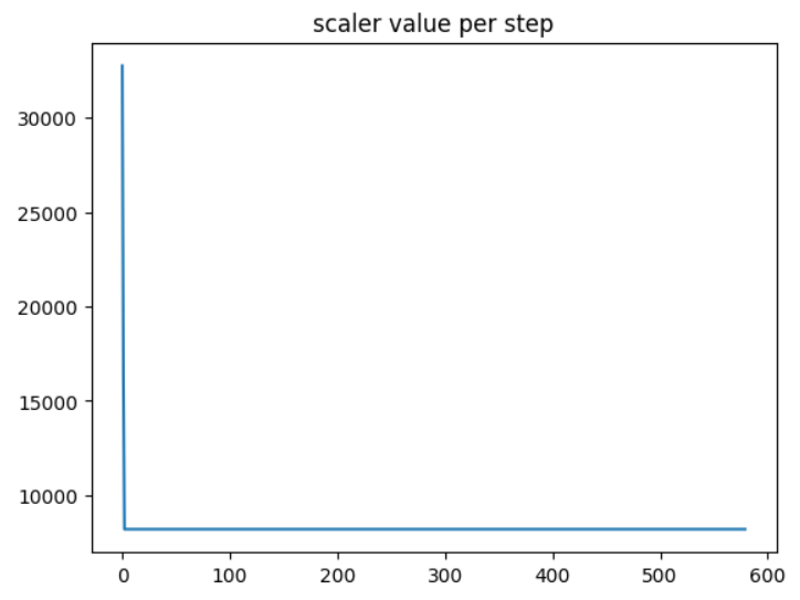
Gradient/loss scaling. The amp library provides automatic gradient scaling techniques so the user doesn’t have to adjust the scaling during training manually. A more detailed algorithm for the scaling factor can be found here.
Once the gradient is scaled, it needs to be scaled back before gradient clipping and regularization. More details can be found here.
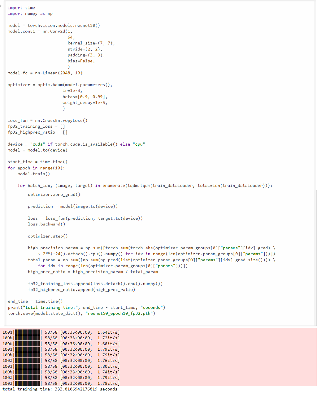
The torch.amp library is relatively easy to use and only requires three lines of code to boost your training speed by 2X.
We start with a very simple task training a ResNet50 model on the FashionMNIST dataset (MIT licence) using FP32; we can see the training time is 333 seconds for ten epochs:

Now that we use the amp library. The amp library only requires three extra lines of code for mixed precision training. We can see the training finished within 141 seconds, which is 2.36X speed up than the FP32 training, while achieving the same precision, recall and F1-score.
scaler = torch.cuda.amp.GradScaler()
# start your training code
# ...
with torch.autocast(device_type="cuda"):
  # training code

# wrapping loss and optimizer
scaler.scale(loss).backward()
scaler.step(optimizer)

scaler.update()
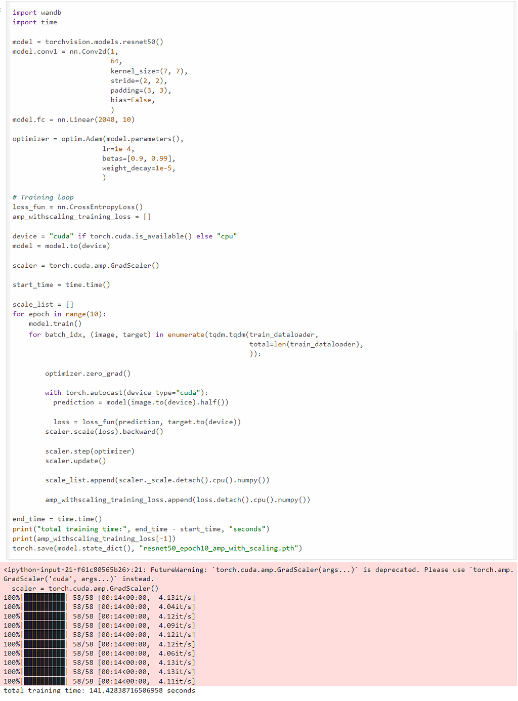

The github link for the code above is here.
Mixed Precision Training is a valuable technique for accelerating deep learning model training. It not only speed up the floating point operations, but also saves the GPU memories as the training batch can be converted to FP16, which saves half the GPU memory. With PyTorch’s amp library, the extra code could be minimized to three additional lines, as the weight copy, loss scaling, operation type casts are all handled by the library internally.
However, mixed precision training doesn’t really resolve the GPU memory issue if the model weight size is much larger than the data batch. For one thing, only certain layers of the model is casted into FP16 while the rest are still calculated in FP32; second, weight update need FP32 copies, which still takes much GPU memory; third, parameters from optimizers like Adam takes much GPU memory during training and the mixed precision training keeps the optimizer parameters unchanged. In that sense, more advanced techniques like DeepSpeed’s ZERO algorithm is needed.
The Mystery Behind the PyTorch Automatic Mixed Precision Library was originally published in Towards Data Science on Medium, where people are continuing the conversation by highlighting and responding to this story.
Originally appeared here:
The Mystery Behind the PyTorch Automatic Mixed Precision Library
Go Here to Read this Fast! The Mystery Behind the PyTorch Automatic Mixed Precision Library
Reflecting on lessons learned using a DB proxy managed by AWS
Originally appeared here:
Setting Up and Monitoring RDS Proxy
Go Here to Read this Fast! Setting Up and Monitoring RDS Proxy


Here are my favorite techniques — one is faster, the other is more accurate.
Originally appeared here:
Building RAGs Without A Retrieval Model Is a Terrible Mistake
Go Here to Read this Fast! Building RAGs Without A Retrieval Model Is a Terrible Mistake


Originally appeared here:
Build RAG-based generative AI applications in AWS using Amazon FSx for NetApp ONTAP with Amazon Bedrock