
Let’s learn the main methods from scipy.stats module in Python.
Originally appeared here:
A Closer Look at Scipy’s Stats Module — Part 2
Go Here to Read this Fast! A Closer Look at Scipy’s Stats Module — Part 2

Let’s learn the main methods from scipy.stats module in Python.
Originally appeared here:
A Closer Look at Scipy’s Stats Module — Part 2
Go Here to Read this Fast! A Closer Look at Scipy’s Stats Module — Part 2


Let’s learn the main methods from scipy.stats module in Python.
Originally appeared here:
A Closer Look at Scipy’s Stats module — Part 1
Go Here to Read this Fast! A Closer Look at Scipy’s Stats module — Part 1

In most common Machine Learning and Natural Language Processing, achieving optimal performance often involves a trade-off between the amount of data used for training and the resulting model accuracy. This blog post explores the concept of sample efficiency in the context of fine-tuning Google’s Gemini Flash model using a PII masking dataset as a practical example. We’ll examine how fine-tuning with increasing amounts of data impacts the tuned model’s capabilities.
What is Sample Efficiency and Why Does it Matter?
Sample efficiency refers to a model’s ability to achieve high accuracy with a limited amount of training data. It’s a key aspect of ML development, especially when dealing with tasks or domains where large, labeled datasets might be scarce or expensive to acquire. A sample-efficient model can learn effectively from fewer examples, reducing the time, cost, and effort associated with data collection and training. LLMs were shown to be very sample efficient, even capable of doing in-context learning with few examples to significantly boost performance. The main motivation of this blog post is to explore this aspect using Gemini Flash as an example. We will evaluate this LLM under different settings and then plot the learning curves to understand how the amount of training data impacts the performance.

Our Experiment: Fine-tuning Gemini Flash for PII masking
To show the impact of sample efficiency, we’ll conduct an experiment focusing on fine-tuning Gemini Flash for PII masking. We’ll use a publicly available PII masking dataset from Hugging Face and evaluate the model’s performance under different fine-tuning scenarios:
For each setting, we’ll evaluate the model’s performance on a fixed test set of 200 sentences, using the BLEU metric to measure the quality of the generated masked text. This metric assesses the overlap between the model’s output and masked sentence, providing a quantitative measure of masking accuracy.
Limitations:
It’s important to acknowledge that the findings of this small experiment might not directly generalize to other use cases or datasets. The optimal amount of data for fine-tuning depends on various factors, including the nature and complexity of the task, the quality of the data, and the specific characteristics of the base model.
My advice here is to take inspiration from the code presented in this post and either:
We will be using a PII (Personal Identifiable Information) masking dataset shared on Huggingface.
The dataset presents two pairs of texts, one original with PII and another one with all PII information masked.
Example:
Input :
A student’s assessment was found on device bearing IMEI: 06–184755–866851–3. The document falls under the various topics discussed in our Optimization curriculum. Can you please collect it?
Target:
A student’s assessment was found on device bearing IMEI: [PHONEIMEI]. The document falls under the various topics discussed in our [JOBAREA] curriculum. Can you please collect it?
The data is synthetic, so no real PII is actually shared here.
Our objective is to build a mapping from the source text to the target text to hide all PII automatically.
Data licence: https://huggingface.co/datasets/ai4privacy/pii-masking-200k/blob/main/license.md
We’ll provide code snippets to facilitate the execution of this experiment. The code will leverage the Hugging Face datasets library for loading the PII masking dataset, the google.generativeai library for interacting with Gemini Flash, and the evaluate library for computing the BLEU score.
pip install transformers datasets evaluate google-generativeai python-dotenv sacrebleu
This snippet installs the required libraries for the project, including:
First, we do data some data loading and splitting:
# Import necessary libraries
from datasets import load_dataset
from google.generativeai.types import HarmCategory, HarmBlockThreshold
# Define GOOGLE_API_KEY as a global variable
# Function to load and split the dataset
def load_data(train_size: int, test_size: int):
    """
    Loads the pii-masking-200k dataset and splits it into train and test sets.
    Args:
        train_size: The size of the training set.
        test_size: The size of the test set.
    Returns:
        A tuple containing the train and test datasets.
    """
    dataset = load_dataset("ai4privacy/pii-masking-200k")
    dataset = dataset["train"].train_test_split(test_size=test_size, seed=42)
    train_d = dataset["train"].select(range(train_size))
    test_d = dataset["test"]
    return train_d, test_d
First, we try zero-shot prompting for this task. This means we explain the task to the LLM and ask it to generate PII masked data from the original text. This is done using a prompt that lists all the tags that need to be masked.
We also parallelize the calls to the LLM api to speed up things a bit.
For the evaluation we use the BLEU score. It is a precision based metric that is commonly used in machine translation to compare the model output to the reference sentence. It has its limitations but is easy to apply and is suited to text-to-text tasks like the one we have at hand.
import google.generativeai as genai
from google.generativeai.types.content_types import ContentDict
from google.generativeai.types import HarmCategory, HarmBlockThreshold

from concurrent.futures import ThreadPoolExecutor
import evaluate

safety_settings = {
    HarmCategory.HARM_CATEGORY_HATE_SPEECH: HarmBlockThreshold.BLOCK_NONE,
    HarmCategory.HARM_CATEGORY_SEXUALLY_EXPLICIT: HarmBlockThreshold.BLOCK_NONE,
    HarmCategory.HARM_CATEGORY_DANGEROUS_CONTENT: HarmBlockThreshold.BLOCK_NONE,
    HarmCategory.HARM_CATEGORY_HARASSMENT: HarmBlockThreshold.BLOCK_NONE,
}
SYS_PROMPT = (
    "Substitute all PII in this text for a generic label like [FIRSTNAME] (Between square brackets)n"
    "Labels to substitute are PREFIX, FIRSTNAME, LASTNAME, DATE, TIME, "
    "PHONEIMEI, USERNAME, GENDER, CITY, STATE, URL, JOBAREA, EMAIL, JOBTYPE, "
    "COMPANYNAME, JOBTITLE, STREET, SECONDARYADDRESS, COUNTY, AGE, USERAGENT, "
    "ACCOUNTNAME, ACCOUNTNUMBER, CURRENCYSYMBOL, AMOUNT, CREDITCARDISSUER, "
    "CREDITCARDNUMBER, CREDITCARDCVV, PHONENUMBER, SEX, IP, ETHEREUMADDRESS, "
    "BITCOINADDRESS, MIDDLENAME, IBAN, VEHICLEVRM, DOB, PIN, CURRENCY, "
    "PASSWORD, CURRENCYNAME, LITECOINADDRESS, CURRENCYCODE, BUILDINGNUMBER, "
    "ORDINALDIRECTION, MASKEDNUMBER, ZIPCODE, BIC, IPV4, IPV6, MAC, "
    "NEARBYGPSCOORDINATE, VEHICLEVIN, EYECOLOR, HEIGHT, SSN, language"
)
# Function to evaluate the zero-shot setting
def evaluate_zero_shot(train_data, test_data, model_name="gemini-1.5-flash"):
    """
    Evaluates the zero-shot performance of the model.
    Args:
        train_data: The training dataset (not used in zero-shot).
        test_data: The test dataset.
        model_name: The name of the model to use.
    Returns:
        The SacreBLEU score for the zero-shot setting.
    """
    model = genai.GenerativeModel(model_name)
    def map_zero_shot(text):
        messages = [
            ContentDict(
                role="user",
                parts=[f"{SYS_PROMPT}nText: {text}"],
            ),
        ]
        response = model.generate_content(messages, safety_settings=safety_settings)
        try:
            return response.text
        except ValueError:
            print(response)
            return ""
    with ThreadPoolExecutor(max_workers=4) as executor:
        predictions = list(
            executor.map(
                map_zero_shot,
                [example["source_text"] for example in test_data],
            )
        )
    references = [[example["target_text"]] for example in test_data]
    sacrebleu = evaluate.load("sacrebleu")
    sacrebleu_results = sacrebleu.compute(
        predictions=predictions, references=references
    )
    print(f"Zero-shot SacreBLEU score: {sacrebleu_results['score']}")
    return sacrebleu_results["score"]
Now, lets try to go further with prompting. In addition to explaining the task to the LLM, we will also show it three examples of what we expect it to do. This usually improves performance.
# Function to evaluate the few-shot setting
def evaluate_few_shot(train_data, test_data, model_name="gemini-1.5-flash"):
    """
    Evaluates the few-shot performance of the model.
    Args:
        train_data: The training dataset.
        test_data: The test dataset.
        model_name: The name of the model to use.
    Returns:
        The SacreBLEU score for the few-shot setting.
    """
    model = genai.GenerativeModel(model_name)
    def map_few_shot(text, examples):
        messages = [
            ContentDict(
                role="user",
                parts=[SYS_PROMPT],
            )
        ]
        for example in examples:
            messages.append(
                ContentDict(role="user", parts=[f"Text: {example['source_text']}"]),
            )
            messages.append(
                ContentDict(role="model", parts=[f"{example['target_text']}"])
            )
        messages.append(ContentDict(role="user", parts=[f"Text: {text}"]))
        response = model.generate_content(messages, safety_settings=safety_settings)
        try:
            return response.text
        except ValueError:
            print(response)
            return ""
    few_shot_examples = train_data.select(range(3))
    with ThreadPoolExecutor(max_workers=4) as executor:
        predictions = list(
            executor.map(
                lambda example: map_few_shot(example["source_text"], few_shot_examples),
                test_data,
            )
        )
    references = [[example["target_text"]] for example in test_data]
    sacrebleu = evaluate.load("sacrebleu")
    sacrebleu_results = sacrebleu.compute(
        predictions=predictions, references=references
    )
    print(f"3-shot SacreBLEU score: {sacrebleu_results['score']}")
    return sacrebleu_results["score"]
Finally, we try fine-tuning. Here, we just use the managed service of the Gemini API. It is free for now so might as well take advantage of it. We use increasing amounts of data and compare the performance of each.
Running a tuning task can’t be easier: we just use the genai.create_tuned_model function with the data, number of epochs and learning rate and parameters.
The training task is asynchronous, which means we don’t have to wait for it. It gets queued and is usually done within 24 hours.
def finetune(train_data, finetune_size, model_name="gemini-1.5-flash"):
    """
    Fine-tunes the model .

    Args:
        train_data: The training dataset.
        finetune_size: The number of samples to use for fine-tuning.
        model_name: The name of the base model to use for fine-tuning.
    Returns:
        The name of the tuned model.
    """
    base_model = f"models/{model_name}-001-tuning"
    tuning_data = [
        {
            "text_input": f"{SYS_PROMPT}nText: {example['source_text']}",
            "output": example["target_text"],
        }
        for example in train_data.select(range(finetune_size))
    ]
    print(len(tuning_data))
    operation = genai.create_tuned_model(
        display_name=f"tuned-{finetune_size}",
        source_model=base_model,
        epoch_count=2,
        batch_size=4,
        learning_rate=0.0001,
        training_data=tuning_data,
    )
You can check the status of the tuning tasks using this code snippet:
import google.generativeai as genai

for model_info in genai.list_tuned_models():
    print(model_info.name)
    print(model_info)
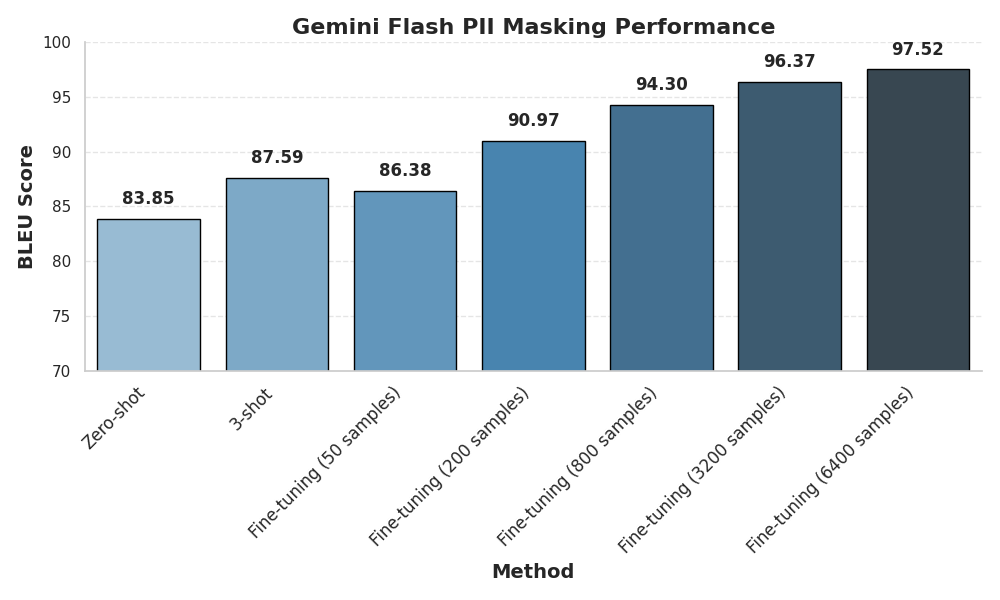
The PII masking algorithm demonstrates increasing performance with the addition of more training data for fine-tuning.
The zero-shot approach achieves a respectable BLEU score of 83.85, indicating a basic understanding of the task even without any training examples. However, providing just three examples (3-shot) improves the score to 87.59, showcasing the effectiveness of even limited examples with in-context learning of LLMs.
Fine-tuning with a small dataset of 50 samples yields a BLEU score of 86.38, slightly lower than the 3-shot approach. However, as the training data increases, the performance improves significantly. With 200 samples, the BLEU score jumps to 90.97, and with 800 samples, it reaches a nice 94.30. The maximum score is reached at the maximum amount of data tested (6400 samples) at 97.52 BLEU score.
The basic conclusion is that, unsurprisingly, you gain performance as you add more data. While the zero-shot and few-shot capabilities of Gemini Flash are impressive, demonstrating its ability to generalize to new tasks, fine-tuning with an big enough amount of data significantly enhances its accuracy. The only unexpected thing here is that few-shot prompting can sometimes outperform fine-tuning if the amount or quality of your training data is too low.
How Much Data Do You Need to Fine-Tune Gemini? was originally published in Towards Data Science on Medium, where people are continuing the conversation by highlighting and responding to this story.
Originally appeared here:
How Much Data Do You Need to Fine-Tune Gemini?
Go Here to Read this Fast! How Much Data Do You Need to Fine-Tune Gemini?


For years I have introduced myself as an analytic methodologist. This aligns with both my formal academic training and my chosen trade. The assertion has been met with confusion, curiosity, and at times disapproval. For many, a methodologist is synonymous with a generalist, which in the world of technology implementation and all eyes on AI, no one much likes to be.
Traditionally, methodologists are those who study research methods, both qualitative and quantitative. The word “research” etymologically speaking means ‘to go about seeking:’ a “creative and systematic work undertaken to increase the stock of knowledge.” (OECD Frascati Manual 2015)
A creative and systematic work…
Practitioner methodologists, independent of their association with research methods, are encyclopedias of ways to approach complex problems. A method is a way of doing something; an approach. I contend that at the nexus of sound science and quality solutioning in any industry is methodology. The remainder of this article advocates for methodology as a discipline.
When designing technical or analytical solutions, we are often working backwards from what we want to achieve. Good science says to put the problem first and then select relevant methods to reach a viable solution. We are to then implement those methods using the corresponding technologies populated with the data that the method(s) require. In other words, data feeds the technologies, technologies implement the methods, and the combination of methods solves the problem.
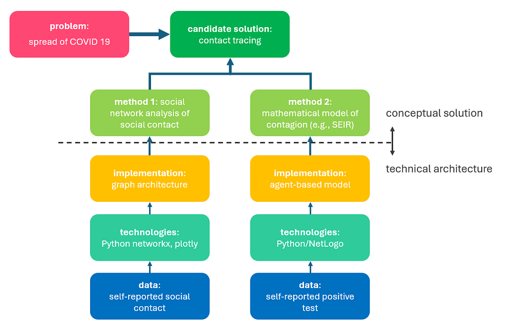
For example, if the problem we are trying to solve is the spread of COVID-19, we may pursue the distillation of a contact tracing solution as outlined in the image below. The candidate solution of contact tracing could involve two methods: 1) social network analysis of contact, and 2) mathematical modeling of contagion (e.g., SEIR model). The technical implementation of these methods will involve selected technologies or software products, and the relevant datasets. The work of designing the conceptual solution is that of methodologists and data scientists. The work of designing the technical architecture is that of solution architects and engineers.
The strength of analytic methodology is in identifying multiple relevant methods to solve a problem and understanding what technical components are required to bring those methods to fruition. It requires both creativity and a systematic process to comprehend multiple approaches, test them quickly, and promote one towards the ultimate solution.
In a research project, this process would be the work of several years and multiple academic publications. In a technical project, this should be the work of a few weeks. It requires a scientific mindset and an agile aptitude for creativity and experimentation.
So what is the relationship between analytic methodology and data science, or “AI/ML?” We see machine learning (ML) and artificial intelligence (AI) getting a lot of attention these days. From a methodology perspective, we are able to put AI (as a domain of science) and ML (as a collection of methods), in their places alongside other technical methods. Even the coveted generative AI is simply an incremental development of unsupervised learning, albeit quite an innovative one.
As a methodologist myself, I always found it odd that ML got so much attention while other methods remained in the shadows of industries (like agent-based modeling…). The Department of Defense found it special enough to create an entirely new organization: the Joint Artificial Intelligence Center (JAIC), now the Chief Digital and Artificial Intelligence Office (CDAO). There are congressionally-appointed funding streams for the application of ML algorithms and generative AI.
I don’t know of another method that has its own congressionally-appointed funding stream. So why is AI so special?
The methodologists’ answer: it’s not. The context-appropriate answer: it’s complex.
ML algorithms handle data volume in a way that humans cannot. In return, they require a lot of computational power. And really good data. Ultimately, ML algorithms are computational implementations of complex math. This means that the results of complex math are now in the hands of analyst users. That, I would argue, is a little special.
ML algorithms can also evolve beyond their intended training or purpose, which is something other methods cannot do. This is the “learning” in machine learning, and the “generative” in generative AI. But the most arresting feature we now see in this class of methods is in language generation. Regardless of the actual capability or comprehension of a large language model (LLM), it speaks our language. And when something speaks to you in your native tongue, something about the experience engenders trust. #anthropomorphism No other method speaks back to the methodologist in plain English.
While these things do make AI a unique domain of science that contains a unique suite of analytic methods, ML algorithms are still methods at the end of the day, and they are not suited to every problem. There is still a need for the methodology mindset in applying these methods where they are fit-for-purpose and applying other methods where they are not.
There are many, many methods from which we methodologists distill creative solutions across industries. I’ve written previously about graph analytics and entity resolution, the first of which is an analytic method, the second of which is more of a data engineering method. There are traditional methods (e.g., simulation, cluster analysis, time series analysis, sentiment analysis). Then, of course, there is machine learning (supervised, unsupervised, and reinforcement learning), and a suite of statistical forecasting methods. There are cognitive thinking strategies (e.g., perspective taking, role playing, analysis of competing hypotheses, multi-criteria decision matrices) and more practitioner-focused capabilities (e.g., geospatial modeling, pattern-of-life analysis, advanced data visualization techniques).
Though by no means exhaustive, these approaches are applied differently from one industry to the next. Ultimately, they are Lego pieces intended for a methodologist to assemble into the grandeur of a solution to whatever challenge the industry or enterprise is facing.
So how do we bring sound science and high-fidelity methodology to quick-turn technical solutioning when there is an imminent deadline?
Too many times we launch data-first efforts. ‘We’ve got these two datasets; what can we learn from them?’ While that is a perfectly valid question to ask of the data within an organization, it isn’t necessarily the best setup for scientifically-grounded inquiry and solutioning.
For accelerated research, rapid prototyping, and quality solutioning, your organization requires the methodology mindset to orient around the problem and begin with the first principles of a solution. Without methodology, inundated with emerging technology, we are all just going faster and further away from the point.
Emerging Tech Is Nothing Without Methodology was originally published in Towards Data Science on Medium, where people are continuing the conversation by highlighting and responding to this story.
Originally appeared here:
Emerging Tech Is Nothing Without Methodology
Go Here to Read this Fast! Emerging Tech Is Nothing Without Methodology


This article offers an explanation of semantic text chunking, a technique designed to automatically group similar pieces of text that can be employed as part of the pre-processing stage of a pipeline for Retrieval Augmented Generation (RAG) or a similar applications. We use visualizations to understand what the chunking is doing, and we explore some extensions that involve clustering and LLM-powered labeling. Check out the full code here.
Automatic information retrieval and summarization of large volumes of text has many useful applications. One of the most well developed is Retrieval Augmented Generation (RAG), which involves extraction of relevant chunks of text from a large corpus — typically via semantic search or some other filtering step — in response to a user question. Then, the chunks are interpreted or summarized by an LLM with the aim of providing a high quality, accurate answer. In order for the extracted chunks to be as relevant as possible to the question its very helpful for them to be semantically coherent, meaning that each chunk is “about” a specific concept and contains a useful packet of information in it’s own right.
Chunking has applications beyond RAG too. Imagine we have a complex document like a book or journal article and want to quickly understand what key concepts it contains. If the text can be clustered into semantically coherent groups and then each cluster summarized in some way, this can really help speed up time to insights. The excellent package BertTopic (see this article for a nice overview) can help here.
Visualization of the chunks can also be insightful, both as a final product and during development. Humans are visual learners in that our brains are much faster at gleaning information from graphs and images rather than streams of text. In my experience, it’s quite difficult to understand what a chunking algorithm has done to the text — and what the optimal parameters might be — without visualizing the chunks in some way or reading them all, which is impractical in the case of large documents.
In this article, we’re going to explore a method to split text into semantically meaningful chunks with an emphasis on using graphs and plots to understand what’s going on. In doing so, we’ll touch on dimensionality reduction and hierarchical clustering of embedding vectors, in addition to the use of LLMs to summarize the chunks so that we can quickly see what information is present. My hope is that this might spark further ideas for anyone researching semantic chunking as a potential tool in their application. I’ll be using Python 3.9, LangChain and Seaborn here, with full details in the repo.
There are a few standard types of chunking and to learn more about them I recommend this excellent tutorial, which also provided inspiration for this article. Assuming we are dealing with English text, the simplest form of chunking is character based, where we choose a fixed window of characters and simply break up the text into chunks of that length. Optionally we can add an overlap between the chunks to preserve some indication of the sequential relationship between them. This is computationally straightforward but there is no guarantee that the chunks will be semantically meaningful or even complete sentences.
Recursive chunking is typically more useful and is seen as the go-to first algorithm for many applications. The process takes in hierarchical list of separators (the default in LangChain is [“nn”, “n”, “ ”, “”] ) and a target length. It then splits up the text using the separators in a recursive way, advancing down the list until each chunk is less than or equal to the target length. This is much better at preserving full paragraphs and sentences, which is good because it makes the chunks much more likely to be coherent. However it does not consider semantics: If one sentence follows on from the last and happens to be at the end of the chunk window, the sentences will be separated.
In semantic chunking, which has implementations in both LangChain and LlamaIndex, the splits are made based on the cosine distance between embeddings of sequential chunks. So we start by dividing the text into small but coherent groups, perhaps using a recursive chunker.
Next we take vectorize each chunk using a model that has been trained to generate meaningful embeddings. Typically this takes the form of a transformer-based bi-encoder (see the SentenceTransformers library for details and examples), or an endpoint such as OpenAI’s text-embeddings-3-small , which is what we use here. Finally, we look at the cosine distances between the embeddings of subsequent chunks and choose breakpoints where the distances are large. Ideally, this helps to create groups of text that are both coherent and semantically distinct.
A recent extension of this called semantic double chunk merging (see this article for details) attempts to extend this by doing a second pass and using some re-grouping logic. So for example if the first pass has put a break between chunks 1 and 2, but chunks 1 and 3 are very similar, it will make a new group that includes chunks 1, 2 and 3. This proves useful if chunk 2 was, for example, a mathematical formula or a code block.
However, when it comes to any type of semantic chunking some key questions remain: How large can the distance between chunk embeddings get before we make a breakpoint, and what do these chunks actually represent? Do we care about that? Answers to these questions depend on the application and the text in question.
Let’s use an example to illustrate the generation of breakpoints using semantic chunking. We will implement our own version of this algorithm, though out of the box implementations are also available as described above. Our demo text is here and it consists of three short, factual essays written by GPT-4o and appended together. The first is about the general importance of preserving trees, the second is about the history of Namibia and the third is a deeper exploration of the importance of protecting trees for medical purposes. The topic choice doesn’t really matter, but the corpus represents an interesting test because the first and third essays are somewhat similar, yet separated by the second which is very different. Each essay is also broken into sections focussing on different things.
We can use a basic RecursiveCharacterTextSplitter to make the initial chunks. The most important parameters here are the chunk size and separators list, and we typically don’t know what they should be without some subject knowledge of the text. Here I chose a relatively small chunk size because I want the initial chunks to be at most a few sentences long. I also chose the separators such that we avoid splitting sentences.
# tools from the text chunking package mentioned in this article
from text_chunking.SemanticClusterVisualizer import SemanticClusterVisualizer
# put your open ai api key in a .env file in the top level of the package
from text_chunking.utils.secrets import load_secrets
# the example text we're talking about
from text_chunking.datasets.test_text_dataset import TestText

# basic splitter
from langchain_text_splitters import RecursiveCharacterTextSplitter
import seaborn as sns
splitter = RecursiveCharacterTextSplitter(
        chunk_size=250,
        chunk_overlap=0,
        separators=["nn", "n", "."],
        is_separator_regex=False
)
Next we can split the text. The min_chunk_len parameter comes into play if any of the chunks generated by the splitter are smaller than this value. If that happens, that chunk just gets appended to the end of the previous one.
original_split_texts = semantic_chunker.split_documents(
    splitter,
    TestText.testing_text,
    min_chunk_len=100,
    verbose=True
)

### Output
# 2024-09-14 16:17:55,014 - Splitting text with original splitter
# 2024-09-14 16:17:55,014 - Creating 53 chunks
# Mean len: 178.88679245283018
# Max len: 245
# Min len: 103
Now we can embed the splits using the embeddings model. You’ll see in the class for SemanticClusterVisualizer that by default we’re using text-embeddings-3-small . This will create a list of 53 vectors, each of length 1536. Intuitively, this means that the semantic meaning of each chunk is represented in a 1536 dimensional space. Not great for visualization, which is why we’ll turn to dimensionality reduction later.
original_split_text_embeddings = semantic_chunker.embed_original_document_splits(original_split_texts)
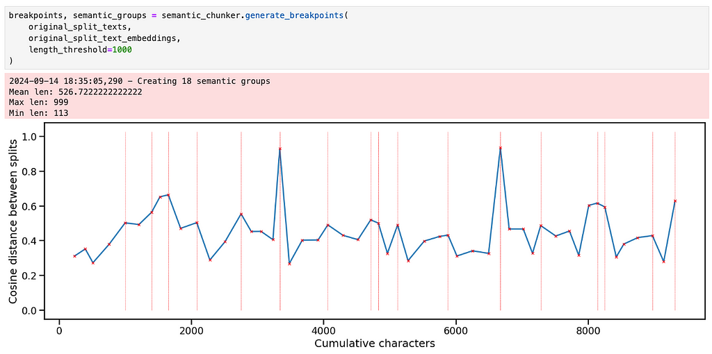
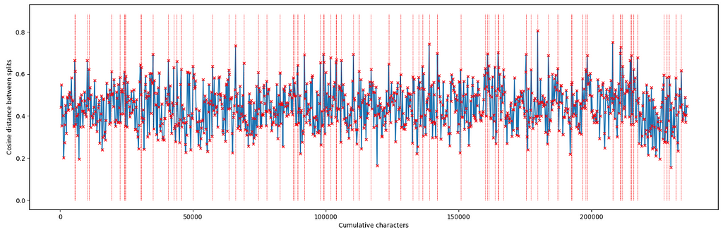
Running the semantic chunker generates a graph like this. We can think of it like a time series, where the x-axis represents distance through the entire text in terms of characters. The y axis represents the cosine distance between the embeddings of subsequent chunks. The break points occur at distances values above the 95th percentile.
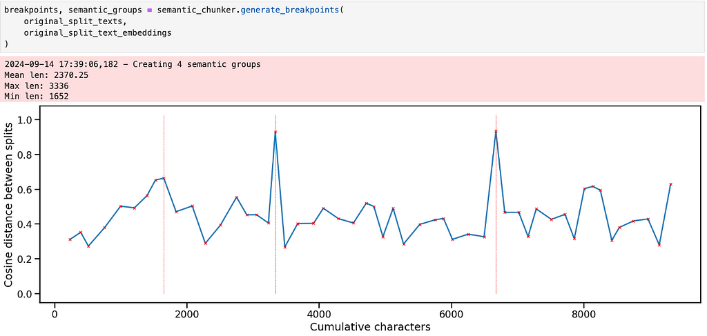
The pattern makes sense given what we know about the text — there are three big subjects, each of which has a few different sections. Aside from the two large spikes though, it’s not clear where the other breakpoints should be.
This is where the subjectivity and iteration comes in — depending on our application, we may want larger or smaller chunks and it’s important to use the graph to help guide our eye towards which chunks to actually read.
There are a few ways we could break the text into more granular chunks. The first is just to decrease the percentile threshold to make a breakpoint.
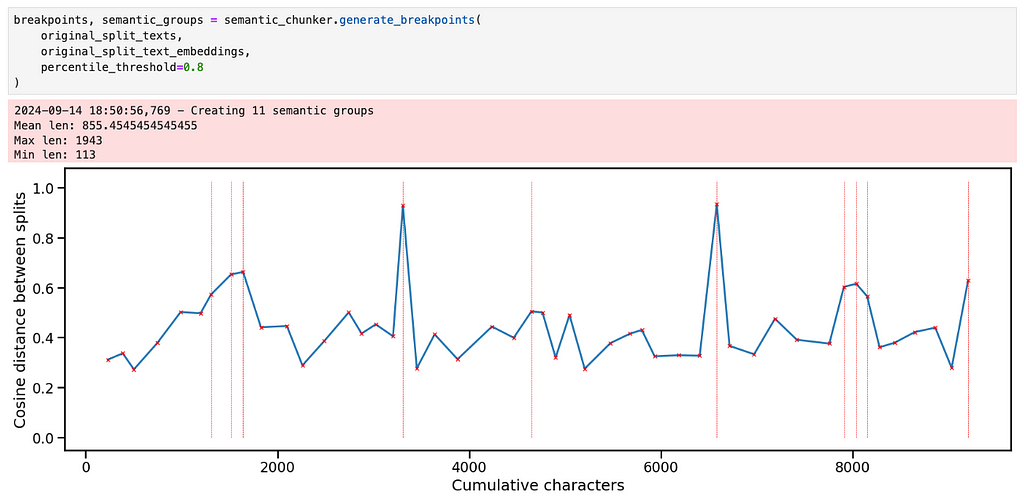
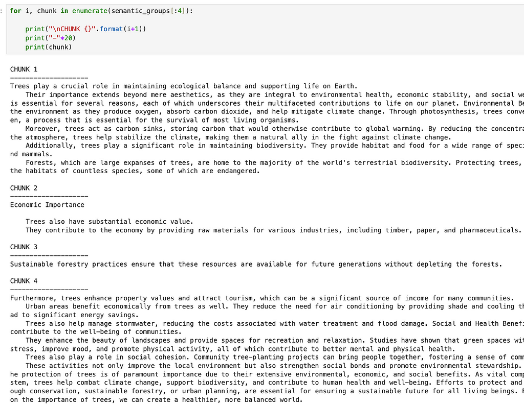
This creates 4 really small chunks and 8 larger ones. If we look at the first 4 chunks, for example, the splits seem semantically reasonable although I would argue that the 4th chunk is a bit too long, given that it contains most of the “economic importance”, “social importance” and “conclusions” sections of the first essay.
Instead of just changing the percentile threshold, an alternative idea is to apply the same threshold recursively. We start by creating breakpoints on the whole text. Then for each newly created chunk, if the chunk is above some length threshold, we create breakpoints just within that chunk. This happens until all the chunks are below the length threshold. Although somewhat subjective, I think this more closely mirrors what a human would do in that they would first identify very different groups of text and then iteratively reduce the size of each one.
It can be implemented with a stack, as shown below.
def get_breakpoints(
    embeddings: List[np.ndarray],
    start: int = 0,
    end: int = None,
    threshold: float = 0.95,
) -> np.ndarray:
    """
    Identifies breakpoints in embeddings based on cosine distance threshold.

    Args:
        embeddings (List[np.ndarray]): A list of embeddings.
        start (int, optional): The starting index for processing. Defaults to 0.
        end (int, optional): The ending index for processing. Defaults to None.
        threshold (float, optional): The percentile threshold for determining significant distance changes. Defaults to 0.95.

    Returns:
        np.ndarray: An array of indices where breakpoints occur.
    """
    if end is not None:
        embeddings_windowed = embeddings[start:end]
    else:
        embeddings_windowed = embeddings[start:]

    len_embeddings = len(embeddings_windowed)
    cdists = np.empty(len_embeddings - 1)

    # get the cosine distances between each chunk and the next one
    for i in range(1, len_embeddings):
        cdists[i - 1] = cosine(embeddings_windowed[i], embeddings_windowed[i - 1])

    # get the breakpoints
    difference_threshold = np.percentile(cdists, 100 * threshold, axis=0)
    difference_exceeding = np.argwhere(cdists >= difference_threshold).ravel()

    return difference_exceeding

def build_chunks_stack(
    self, length_threshold: int = 20000, cosine_distance_percentile_threshold: float = 0.95
) -> np.ndarray:
    """
    Builds a stack of text chunks based on length and cosine distance thresholds.

    Args:
        length_threshold (int, optional): Minimum length for a text chunk to be considered valid. Defaults to 20000.
        cosine_distance_percentile_threshold (float, optional): Cosine distance percentile threshold for determining breakpoints. Defaults to 0.95.

    Returns:
        np.ndarray: An array of indices representing the breakpoints of the chunks.
    """

    # self.split texts are the original split texts
    # self.split text embeddings are their embeddings
    S = [(0, len(self.split_texts))]
    all_breakpoints = set()
    while S:
        # get the start and end of this chunk
        id_start, id_end = S.pop()

        # get the breakpoints for this chunk
        updated_breakpoints = self.get_breakpoints(
            self.split_text_embeddings,
            start=id_start,
            end=id_end,
            threshold=cosine_distance_percentile_threshold,
        )
        updated_breakpoints += id_start

        # add the updated breakpoints to the set
        updated_breakpoints = np.concatenate(
            (np.array([id_start - 1]), updated_breakpoints, np.array([id_end]))
        )

        # for each updated breakpoint, add its bounds to the set and
        # to the stack if it is long enough
        for index in updated_breakpoints:
            text_group = self.split_texts[id_start : index + 1]
            if (len(text_group) > 2) and (
                self.get_text_length(text_group) >= length_threshold
            ):
                S.append((id_start, index))
            id_start = index + 1
        all_breakpoints.update(updated_breakpoints)

    # get all the breakpoints except the start and end (which will correspond to the start
    # and end of the text splits)
    return np.array(sorted(all_breakpoints))[1:-1]
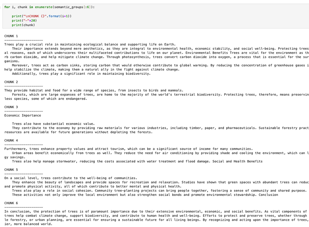
Our choice of length_threshold is also subjective and can be informed by the plot. In this case, a threshold of 1000 appears to work well. It divides the essays quite nicely into short and meaningfully different chunks.
Looking at the chunks corresponding to the first essay, we see that they are closely aligned with the different sections that GPT4-o created when it wrote the essay. Obviously in the case of this particular essay we could have just split on “nn” and been done here, but we want a more general approach.
Now that we have made some candidate semantic chunks, it might be useful to see how similar they are to one another. This will help us get a sense for what information they contain. We will proceed by embedding the semantic chunks, and then use UMAP to reduce the dimensionality of the resulting embeddings to 2D so that we can plot them.
UMAP stands for Uniform Manifold Approximation and Projection, and is a powerful, general dimensionality reduction technique that can capture non-linear relationships. A full explanation of how it works can be found here. The purpose of using it here is to capture something of the relationships that exist between the embedded chunks in 1536-D space in a 2-D plot
from umap import UMAP

dimension_reducer = UMAP(
            n_neighbors=5,
            n_components=2,
            min_dist=0.0,
            metric="cosine",
            random_state=0
)
reduced_embeddings = dimension_reducer.fit_transform(semantic_embeddings)

splits_df = pd.DataFrame(
            {
                "reduced_embeddings_x": reduced_embeddings[:, 0],
                "reduced_embeddings_y": reduced_embeddings[:, 1],
                "idx": np.arange(len(reduced_embeddings[:, 0])),
            }
)

splits_df["chunk_end"] = np.cumsum([len(x) for x in semantic_text_groups])

ax = splits_df.plot.scatter(
            x="reduced_embeddings_x",
            y="reduced_embeddings_y",
            c="idx",
            cmap="viridis"
)

ax.plot(
            reduced_embeddings[:, 0],
            reduced_embeddings[:, 1],
            "r-",
            linewidth=0.5,
            alpha=0.5,
)
UMAP is quite sensitive to the n_neighbors parameter. Generally the smaller the value of n_neighbors, the more the algorithm focuses on the use of local structure to learn how to project the data into lower dimensions. Setting this value too small can lead to projections that don’t do a great job of capturing the large scale structure of the data, and it should generally increase as the number of datapoints grows.
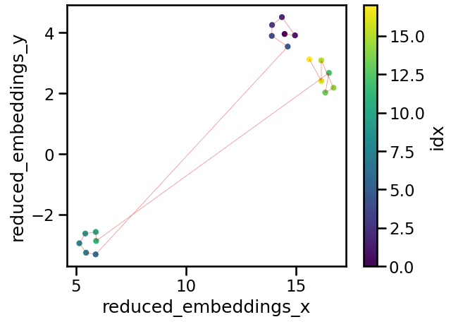
A projection of our data is shown below and its quite informative: Clearly we have three clusters of similar meaning, with the 1st and 3rd being more similar to each other than either is to the 2nd. The idx color bar in the plot above shows the chunk number, while the red line gives us an indication of the sequence of the chunks.
What about automatic clustering? This would be helpful if we wanted to group the chunks into larger segments or topics, which could serve as useful metadata to filter on in a RAG application with hybrid search, for example. We also might be able to group chunks that are far apart in the text (and therefore would not have been grouped by the standard semantic chunking in section 1) but have similar meanings.
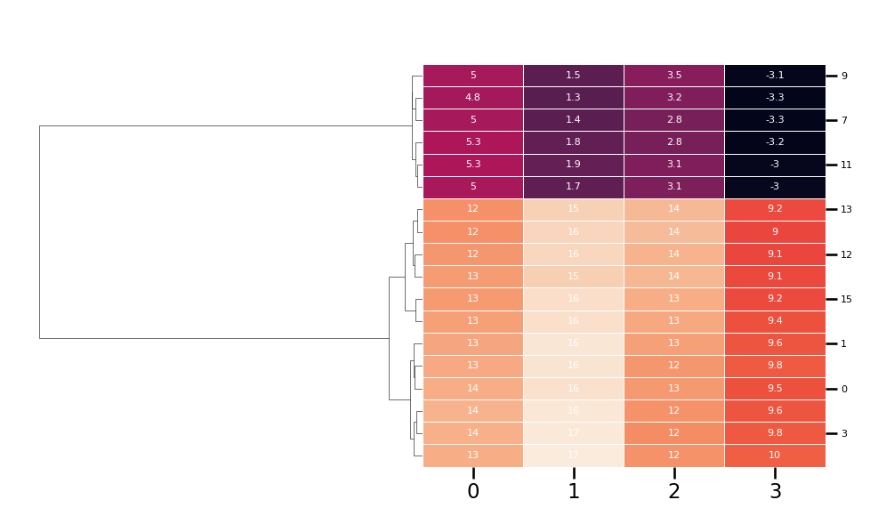
There are many clustering approaches that could be used here. HDBSCAN is a possibility, and is the default method recommended by the BERTopic package. However, in this case hierarchical clustering seems more useful since it can give us a sense of the relative importance of whatever groups emerge. To run hierarchical clustering, we first use UMAP to reduce the dimensionality of the dataset to a smaller number of components. So long as UMAP is working well here, the exact number of components shouldn’t significantly affect the clusters that get generated. Then we use the hierarchy module from scipy to perform the clustering and plot the result using seaborn
from scipy.cluster import hierarchy
from scipy.spatial.distance import pdist
from umap import UMAP
import seaborn as sns

# set up the UMAP
dimension_reducer_clustering = UMAP(
            n_neighbors=umap_neighbors,
            n_components=n_components_reduced,
            min_dist=0.0,
            metric="cosine",
            random_state=0
)
reduced_embeddings_clustering = dimension_reducer_clustering.fit_transform(
    semantic_group_embeddings
)

# create the hierarchy
row_linkage = hierarchy.linkage(
    pdist(reduced_embeddings_clustering),
    method="average",
    optimal_ordering=True,
)

# plot the heatmap and dendogram
g = sns.clustermap(
    pd.DataFrame(reduced_embeddings_clustering),
    row_linkage=row_linkage,
    row_cluster=True,
    col_cluster=False,
    annot=True,
    linewidth=0.5,
    annot_kws={"size": 8, "color": "white"},
    cbar_pos=None,
    dendrogram_ratio=0.5
)

g.ax_heatmap.set_yticklabels(
  g.ax_heatmap.get_yticklabels(), rotation=0, size=8
)
The result is also quite informative. Here n_components_reduced was 4, so we reduced the dimensionality of the embeddings to 4D, therefore making a matrix with 4 features where each row represents one of the semantic chunks. Hierarchical clustering has identified the two major groups (i.e. trees and Namibia), two large subgroup within trees (i.e. medical uses vs. other) and an number of other groups that might be worth exploring.
Note that BERTopic uses a similar technique for topic visualization, which could be seen as an extension of what’s being presented here.
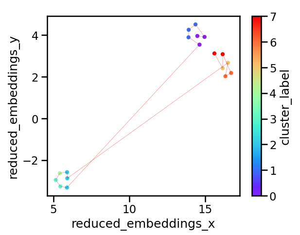
How is this useful in our exploration of semantic chunking? Depending on the results, we may choose to group some of the chunks together. This is again quite subjective and it might be important to try out a few different types of grouping. Let’s say we looked at the dendrogram and decided we wanted 8 distinct groups. We could then cut the hierarchy accordingly, return the cluster labels associated with each group and plot them.
cluster_labels = hierarchy.cut_tree(linkage, n_clusters=n_clusters).ravel()
dimension_reducer = UMAP(
  n_neighbors=umap_neighbors,
  n_components=2,
  min_dist=0.0,
  metric="cosine",
  random_state=0
)
reduced_embeddings = dimension_reducer.fit_transform(semantic_embeddings)

splits_df = pd.DataFrame(
            {
                "reduced_embeddings_x": reduced_embeddings[:, 0],
                "reduced_embeddings_y": reduced_embeddings[:, 1],
                "cluster_label": cluster_labels,
            }
        )

splits_df["chunk_end"] = np.cumsum(
            [len(x) for x in semantic_text_groups]
        ).reshape(-1, 1)

ax = splits_df.plot.scatter(
            x="reduced_embeddings_x",
            y="reduced_embeddings_y",
            c="cluster_label",
            cmap="rainbow",
        )

ax.plot(
  reduced_embeddings[:, 0],
  reduced_embeddings[:, 1],
  "r-",
  linewidth=0.5,
  alpha=0.5,
)
The resulting plot is shown below. We have 8 clusters, and their distribution in the 2D space looks reasonable. This again demonstrates the importance of visualization: Depending on the text, application and stakeholders, the right number and distribution of groups will likely be different and the only way to check what the algorithm is doing is by plotting graphs like this.
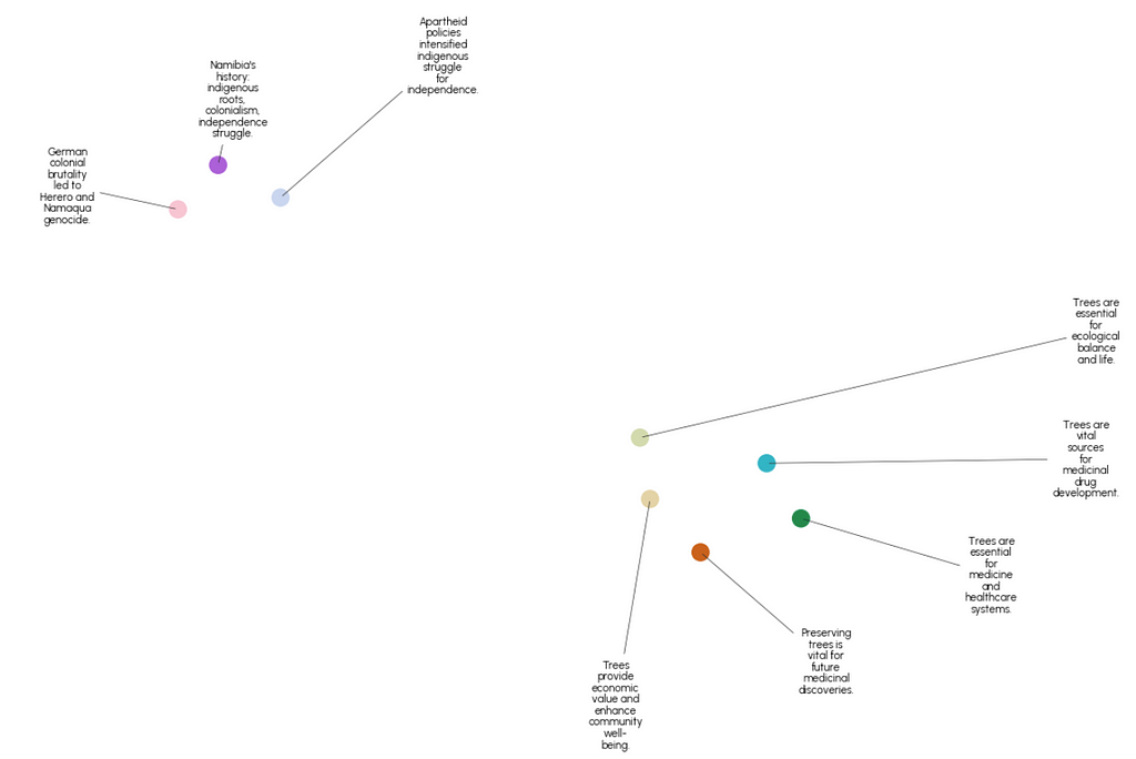
Assume after a few iterations of the steps above, we’ve settled on semantic splits and clusters that we’re happy with. It then makes sense to ask what these clusters actually represent? Obviously we could read the text and find out, but for a large corpus this is impractical. Instead, let’s use an LLM to help. Specifically, we will feed the text associated with each cluster to GPT-4o-mini and ask it to generate a summary. This is a relatively simple task with LangChain, and the core aspects of the code are shown below
import langchain
from langchain.prompts import PromptTemplate
from langchain_core.output_parsers.string import StrOutputParser
from langchain.callbacks import get_openai_callback
from dataclasses import dataclass


@dataclass
class ChunkSummaryPrompt:
    system_prompt: str = """
        You are an expert at summarization and information extraction from text. You will be given a chunk of text from a document and your
        task is to summarize what's happening in this chunk using fewer than 10 words.

        Read through the entire chunk first and think carefully about the main points. Then produce your summary.

        Chunk to summarize: {current_chunk}
    """

    prompt: langchain.prompts.PromptTemplate = PromptTemplate(
        input_variables=["current_chunk"],
        template=system_prompt,
    )

class ChunkSummarizer(object):
    def __init__(self, llm):
        self.prompt = ChunkSummaryPrompt()
        self.llm = llm
        self.chain = self._set_up_chain()

    def _set_up_chain(self):
        return self.prompt.prompt | self.llm | StrOutputParser()

    def run_and_count_tokens(self, input_dict):
        with get_openai_callback() as cb:
            result = self.chain.invoke(input_dict)

        return result, cb

llm_model = "gpt-4o-mini"
llm = ChatOpenAI(model=llm_model, temperature=0, api_key=api_key)
summarizer = ChunkSummarizer(llm)
Running this on our 8 clusters and plotting the result with datamapplot gives the following
An alternative way of visualizing these groups is similar to the graphs shown in section 2, where we plot cumulative character number on the x axis and show the boundaries between the groups. Recall that we had 18 semantic chunks and have now grouped them further into 8 clusters. Plotting them like this shows how the semantic content of the text changes from beginning to end, highlights the fact that similar content is not always adjacent and gives a visual indication of the relative size of the chunks.
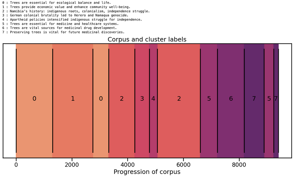
The code used to produce these figures can be found here.
So far we’ve tested this workflow on a relatively small amount of text for demo purposes. Ideally it would also be useful on a larger corpus without significant modification. To test this, let’s try it out on a book downloaded from Project Gutenberg, and I’ve chosen the Wizard of Oz here. This is a much more difficult task because novels are typically not arranged in clear semantically distinct sections like factual essays. Although they are commonly arranged in chapters, the story line may “arch” in a continuous fashion, or skip around between different subjects. It would be very interesting to see if semantic chunk analysis could be used to learn something about the style of different authors from their work.
from text_chunking.SemanticClusterVisualizer import SemanticClusterVisualizer
from text_chunking.utils.secrets import load_secrets
from text_chunking.datasets.test_text_dataset import TestText, TestTextNovel
from langchain_text_splitters import RecursiveCharacterTextSplitter

secrets = load_secrets()
semantic_chunker = SemanticClusterVisualizer(api_key=secrets["OPENAI_API_KEY"])

splitter = RecursiveCharacterTextSplitter(
        chunk_size=250,
        chunk_overlap=0,
        separators=["nn", "n", "."],
        is_separator_regex=False
)

original_split_texts = semantic_chunker.split_documents(
    splitter,
    TestTextNovel.testing_text,
    min_chunk_len=100,
    verbose=True
)
original_split_text_embeddings = semantic_chunker.embed_original_document_splits(original_split_texts)

breakpoints, semantic_groups = semantic_chunker.generate_breakpoints(
    original_split_texts,
    original_split_text_embeddings,
    length_threshold=10000 #may need some iteration to find a good value for this parameter
)
This generates 77 semantic chunks of varying size. Doing some spot checks here led me to feel confident that it was working relatively well and many of the chunks end up being divided on or close to chapter boundaries, which makes a lot of sense.
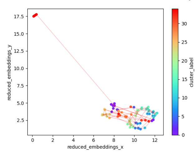
On looking at the hierarchical clustering dendrogram, I decided to experiment with reduction to 35 clusters. The result reveals an outlier in the top left of the plot below (cluster id 34), which turns out to be a group of chunks at the very end of the text that contain a lengthy description of the terms under which the book is distributed.
The descriptions given to each of the clusters are shown below and, with the exception of the first one, they provide a nice overview of the main events of the novel. A quick check on the actual texts associated with each one confirms that they are reasonably accurate summaries, although again, a determination of where the boundaries of the clusters should be is very subjective.
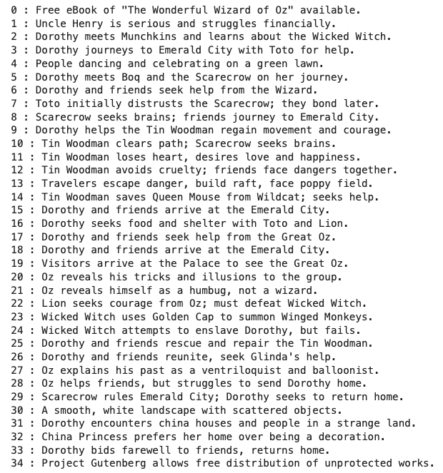
GPT-4o-mini labeled the outlier cluster “Project Gutenberg allows free distribution of unprotected works”. The text associated with this label is not particularly interesting to us, so let’s remove it and re-plot the result. This will make the structure in the novel easier to see.
What if we are interested in larger clusters? If we were to focus on high level structure, the dendrogram suggests approximately six clusters of semantic chunks, which are plotted below.
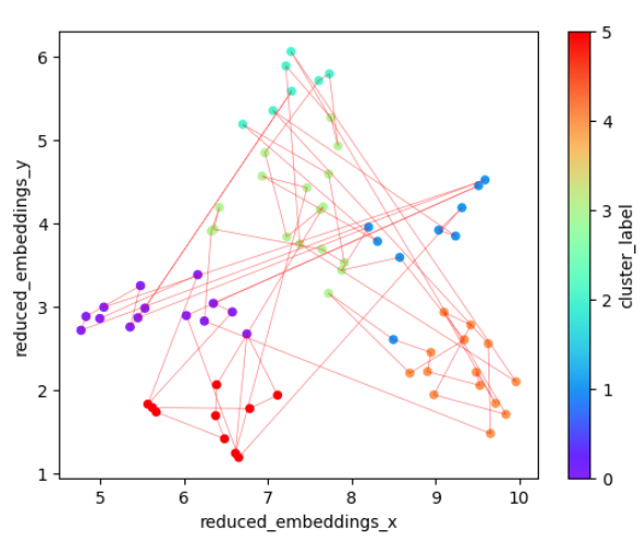
There’s a lot of jumping back and forth between points that are somewhat distant in this semantic space, suggesting frequent sudden changes in subject. It’s also interesting to consider the connectivity between the various clusters: 4 and 5 have no links between them for example, while there’s a lot of back and forth between 0 and 1.
Can we summarize these larger clusters? It turns out that our prompt doesn’t seem well suited for chunks of this size, producing descriptions that seem either too specific to one part of the cluster (i.e. clusters 0 and 4) or too vague to be very helpful. Improved prompt engineering — possibly involving multiple summarization steps — would probably improve the results here.
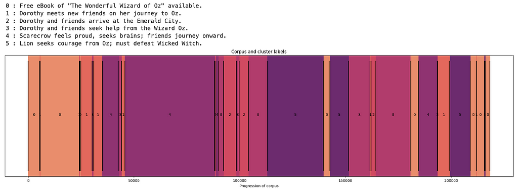
Despite the unhelpful names, this plot of the text segments colored by cluster is still informative as a guide to selective reading of the text. We see that the book starts and ends on the same cluster, which likely is about descriptions of Dorothy, Toto and their home — and aligns with the story arch of the Wizard of Oz as a journey and subsequent return. Cluster 1 is mainly about meeting new characters, which happens mainly near the beginning but also periodically throughout the book. Clusters 2 and 3 are concerned with Emerald City and the Wizard, while clusters 4 and 5 are broadly about journeying and fighting respectively.
Thanks for making it to the end! Here we took a deep dive into the idea of semantic chunking, and how it can be complimented by dimensionality reduction, clustering and visualization. The major takeaway is the importance of systematically exploring the effects of different chunking techniques and a parameters on your text before deciding on the most suitable approach. My hope is that this article will spark new ideas about how we can use AI and visualization tools to advance semantic chunking and quickly extract insights from large bodies of text. Please feel free to explore the full codebase here https://github.com/rmartinshort/text_chunking.
A Visual Exploration of Semantic Text Chunking was originally published in Towards Data Science on Medium, where people are continuing the conversation by highlighting and responding to this story.
Originally appeared here:
A Visual Exploration of Semantic Text Chunking
Go Here to Read this Fast! A Visual Exploration of Semantic Text Chunking
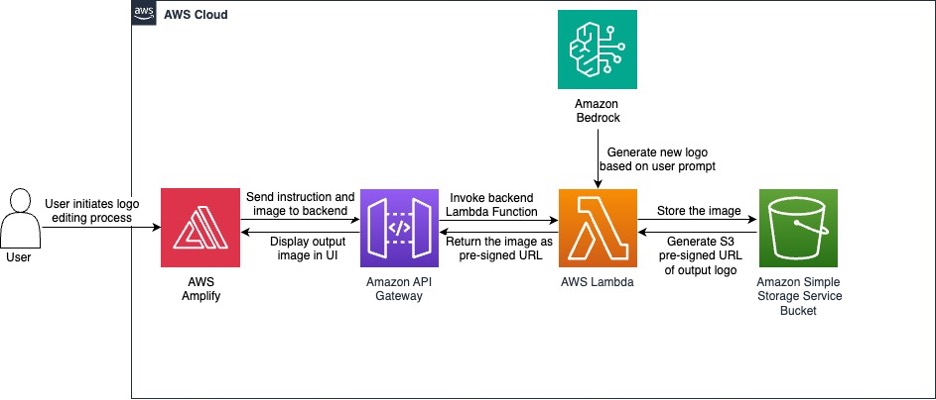

Originally appeared here:
Revolutionize logo design creation with Amazon Bedrock: Embracing generative art, dynamic logos, and AI collaboration


Originally appeared here:
Reinvent personalization with generative AI on Amazon Bedrock using task decomposition for agentic workflows

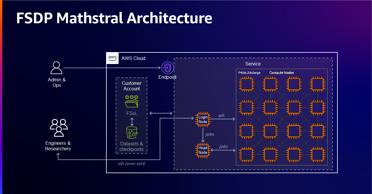
Originally appeared here:
Accelerate pre-training of Mistral’s Mathstral model with highly resilient clusters on Amazon SageMaker HyperPod
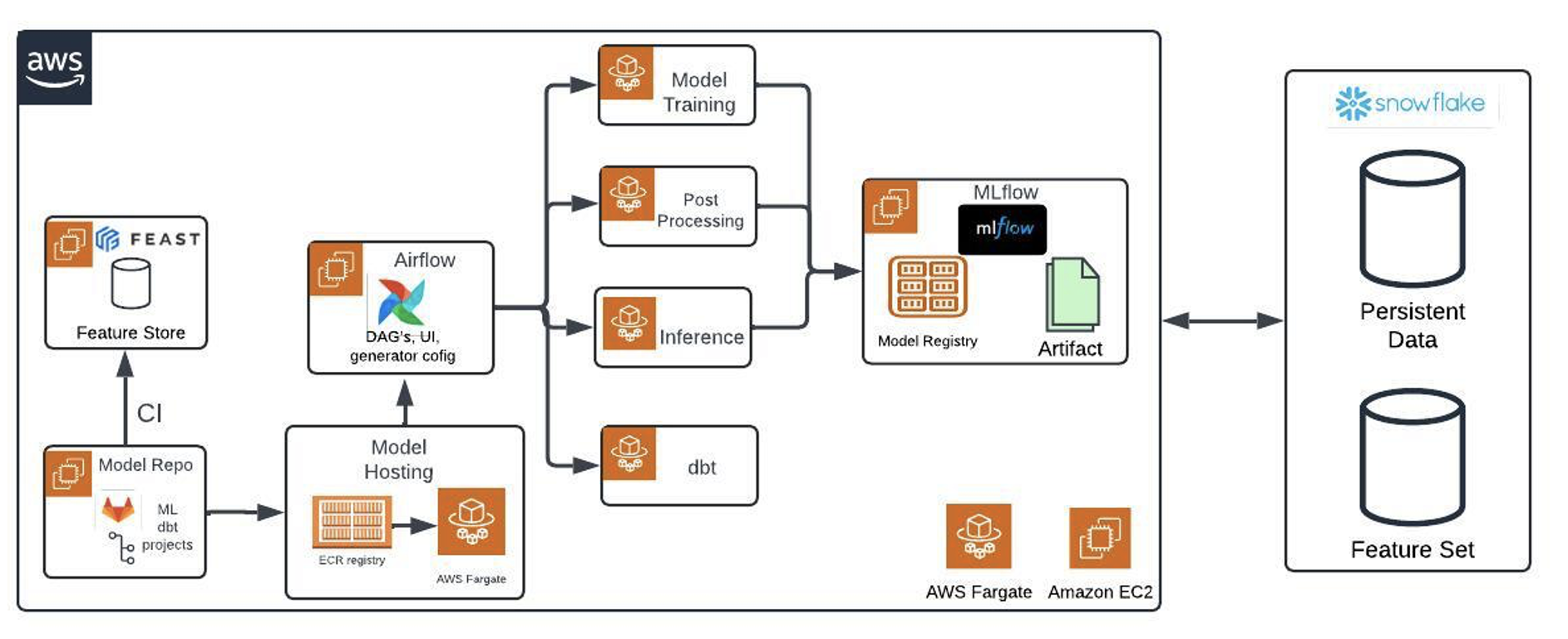

Originally appeared here:
Building an efficient MLOps platform with OSS tools on Amazon ECS with AWS Fargate
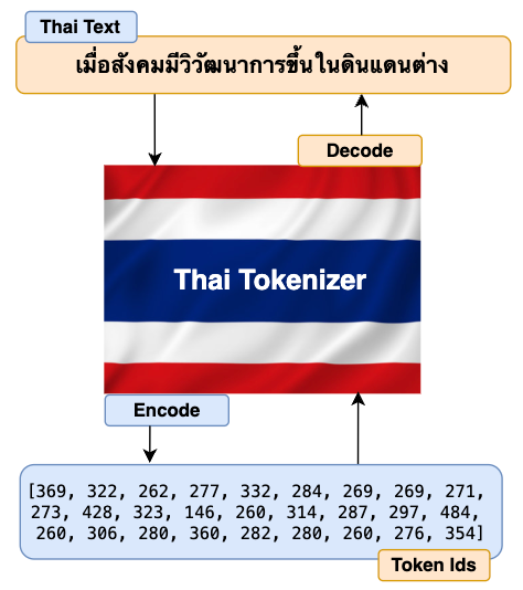

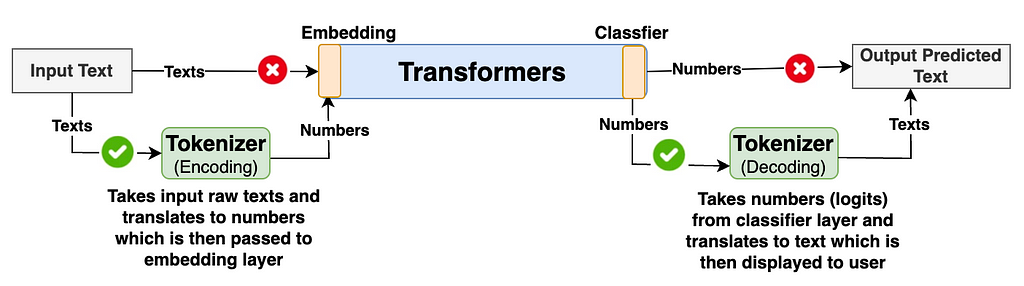
The primary task of the Tokenizer is to translate the raw input texts (Thai in our case but can be in any foreign language) into numbers and pass them to the model’s transformers. The model’s transformer then generates output as numbers. Again, Tokenizer translates these numbers back to texts which is understandable to end users. The high level diagram below describes the flow explained above.
Generally, many of us are only interested in learning how the model’s transformer architecture works under the hood. We often overlook learning some important components such as tokenizers in detail. Understanding how tokenizer works under the hood and having good control of its functionalities gives us good leverage to improve our model’s accuracy and performance.
Similar to Tokenizer, some of the most important components of LLM implementation pipelines are Data preprocessing, Evaluation, Guardrails/Security, and Testing/Monitoring. I would highly recommend you study more details on these topics. I realized the importance of these components only after I was working on the actual implementation of my foundational multilingual model ThaiLLM in production.
The good news is that after you finish building Thai Tokenizer, you can easily build a tokenizer in any other language. All the building steps are the same except that you’ll have to train on the dataset of your choice of language.
Now that we’ve all the good reason to build our own tokenizer. Below are steps to building our tokenizer in the Thai language.
The BPE algorithm is used in many popular LLMs such as Llama, GPT, and others to build their tokenizer. We can choose one of these LLM tokenizers if our model is based on the English language. Since we’re building the Thai Tokenizer, the best option is to create our own BPE algorithm from scratch and use it to build our tokenizer. Let’s first understand how the BPE algorithm works with the help of the simple flow diagram below and then we’ll start building it accordingly.
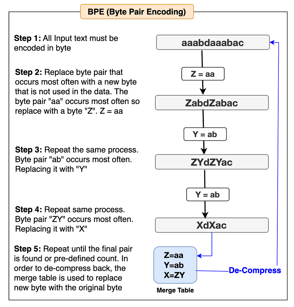
The examples in the flow diagram are shown in English to make it easier to understand.
Let’s write code to implement the BPE algorithm for our Thai Tokenizer.
# A simple practice example to get familiarization with utf-8 encoding to convert strings to bytes.
text = "How are you คุณเป็นอย่างไร"      # Text string in both English and Thai
text_bytes = text.encode("utf-8")
print(f"Text in byte: {text_bytes}")

text_list = list(text_bytes)          # Converts text bytes to a list of integer
print(f"Text list in integer: {text_list}")
# As I don't want to reinvent the wheel, I will be referencing most of the code block from Andrej Karpathy's GitHub (https://github.com/karpathy/minbpe?tab=readme-ov-file).
# However, I'll be modifying code blocks specific to building our Thai language tokenizer and also explaining the codes so that you can understand how each code block works and make it easy when you implement code for your use case later.

# This module provides access to the Unicode Character Database (UCD) which defines character properties for all Unicode characters.
import unicodedata

# This function returns a dictionary with consecutive pairs of integers and their counts in the given list of integers.
def get_stats(ids, stats=None):

    stats = {} if stats is None else stats
    # zip function allows to iterate consecutive items from given two list
    for pair in zip(ids, ids[1:]):
        # If a pair already exists in the stats dictionary, add 1 to its value else assign the value as 0.
        stats[pair] = stats.get(pair, 0) + 1
    return stats

# Once we find out the list of consecutive pairs of integers, we'll then replace those pairs with new integer tokens.
def merge(ids, pair, idx):
    newids = []
    i = 0
    # As we'll be merging a pair of ids, hence the minimum id in the list should be 2 or more.
    while i < len(ids):
        # If the current id and next id(id+1) exist in the given pair, and the position of id is not the last, then replace the 2 consecutive id with the given index value.
        if ids[i] == pair[0] and i < len(ids) - 1 and ids[i+1] == pair[1]:
            newids.append(idx)
            i += 2  # If the pair is matched, the next iteration starts after 2 positions in the list.
        else:
            newids.append(ids[i])
            i += 1  # Since the current id pair didn't match, so start iteration from the 1 position next in the list.
    # Returns the Merged Ids list
    return newids

# This function checks that using 'unicodedata.category' which returns "C" as the first letter if it is a control character and we'll have to replace it readable character.
def replace_control_characters(s: str) -> str:
    chars = []
    for ch in s:
        # If the character is not distorted (meaning the first letter doesn't start with "C"), then append the character to chars list.
        if unicodedata.category(ch)[0] != "C":
            chars.append(ch)
        # If the character is distorted (meaning the first letter has the letter "C"), then replace it with readable bytes and append to chars list.
        else:
            chars.append(f"\u{ord(ch):04x}")
    return "".join(chars)

# Some of the tokens such as control characters like Escape Characters can't be decoded into valid strings.
# Hence those need to be replace with readable character such as �
def render_token(t: bytes) -> str:
    s = t.decode('utf-8', errors='replace')
    s = replace_control_characters(s)
    return s
The two functions get_stats and merge defined above in the code block are the implementation of the BPE algorithm for our Thai Tokenizer. Now that the algorithm is ready. Let’s write code to train our tokenizer.
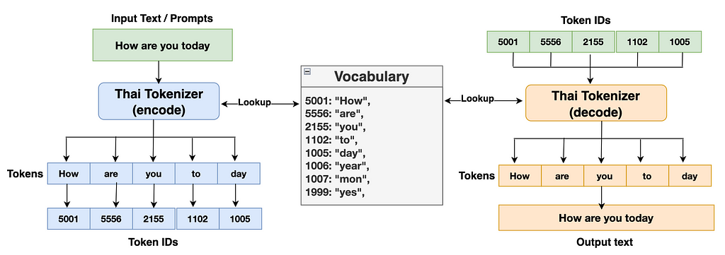
Training tokenizer involves generating a vocabulary which is a database of unique tokens (word and sub-words) along with a unique index number assigned to each token. We’ll be using the Thai Wiki dataset from the Hugging Face to train our Thai Tokenizer. Just like training an LLM requires a huge data, you’ll also require a good amount of data to train a tokenizer. You could also use the same dataset to train the LLM as well as tokenizer though not mandatory. For a multilingual LLM, it is advisable to use both the English and Thai datasets in the ratio of 2:1 which is a standard approach many practitioners follow.
Let’s begin writing the training code.
# Import Regular Expression
import regex as re

# Create a Thai Tokenizer class.
class ThaiTokenizer():

  def __init__(self):

        # The byte pair should be done within the related words or sentences that give a proper context. Pairing between unrelated words or sentences may give undesirable output.
        # To prevent this behavior, we'll implement the LLama 3 regular expression pattern to make meaningful chunks of our text before implementing the byte pair algorithm.
        self.pattern = r"(?i:'s|'t|'re|'ve|'m|'ll|'d)|[^rnp{L}p{N}]?p{L}+|p{N}{1,3}| ?[^sp{L}p{N}]+[rn]*|s*[rn]+|s+(?!S)|s+"
        self.compiled_pattern = re.compile(self.pattern)

        # Special tokens are used to provide coherence in the sequence while training.
        # Special tokens are assigned a unique index number and stored in vocabulary.
        self.special_tokens = {
            '<|begin_of_text|>': 1101,
            '<|end_of_text|>': 1102,
            '<|start_header_id|>': 1103,
            '<|end_header_id|>': 1104,
            '<|eot_id|>': 1105
        }

        # Initialize merges with empty dictionary
        self.merges = {}

        # Initialize the vocab dictionary by calling the function _build_vocab which is defined later in this class.
        self.vocab = self._build_vocab()

  # Tokenizer training function
  def train(self, text, vocab_size):

        # Make sure the vocab size must be at least 256 as the utf-8 encoding for the range 0-255 are same as the Ascii character.
        assert vocab_size >= 256
        # Total number of merges into the vocabulary.
        num_merges = vocab_size - 256

        # The first step is to make sure to split the text up into text chunks using the pattern defined above.
        text_chunks = re.findall(self.compiled_pattern, text)

        # Each text_chunks will be utf-8 encoded to bytes and then converted into an integer list.
        ids = [list(ch.encode("utf-8")) for ch in text_chunks]

        # Iteratively merge the most common pairs to create new tokens
        merges = {} # (int, int) -> int
        vocab = {idx: bytes([idx]) for idx in range(256)} # idx -> bytes

        # Until the total num_merges is reached, find the common pair of consecutive id in the ids list and start merging them to create a new token
        for i in range(num_merges):
            # Count the number of times every consecutive pair appears
            stats = {}
            for chunk_ids in ids:
                # Passing in stats will update it in place, adding up counts
                get_stats(chunk_ids, stats)
            # Find the pair with the highest count
            pair = max(stats, key=stats.get)
            # Mint a new token: assign it the next available id
            idx = 256 + i
            # Replace all occurrences of pair in ids with idx
            ids = [merge(chunk_ids, pair, idx) for chunk_ids in ids]
            # Save the merge
            merges[pair] = idx
            vocab[idx] = vocab[pair[0]] + vocab[pair[1]]

        # Save class variables to be used later during tokenizer encode and decode
        self.merges = merges
        self.vocab = vocab

  # Function to return a vocab dictionary combines with merges and special tokens
  def _build_vocab(self):
        # The utf-8 encoding for the range 0-255 are same as the Ascii character.
        vocab = {idx: bytes([idx]) for idx in range(256)}

        # Iterate through merge dictionary and add into vocab dictionary
        for (p0, p1), idx in self.merges.items():
            vocab[idx] = vocab[p0] + vocab[p1]

        # Iterate through special token dictionary and add into vocab dictionary
        for special, idx in self.special_tokens.items():
            vocab[idx] = special.encode("utf-8")

        return vocab

  # After training is complete, use the save function to save the model file and vocab file.
  # Model file will be used to load the tokenizer model for further use in llm
  # Vocab file is just for the purpose of human verification
  def save(self, file_prefix):
        # Writing to model file
        model_file = file_prefix + ".model"           # model file name

        # Model write begins
        with open(model_file, 'w') as f:
            f.write("thai tokenizer v1.0n")          # write the tokenizer version
            f.write(f"{self.pattern}n")              # write the pattern used in tokenizer
            f.write(f"{len(self.special_tokens)}n")  # write the length of special tokens

            # Write each special token in the specific format like below
            for tokens, idx in self.special_tokens.items():
                f.write(f"{tokens} {idx}n")

            # Write only the keys part from the merges dict
            for idx1, idx2 in self.merges:
                f.write(f"{idx1} {idx2}n")

        # Writing to the vocab file
        vocab_file = file_prefix + ".vocab"       # vocab file name

        # Change the position of keys and values of merge dict and store into inverted_merges
        inverted_merges = {idx: pair for pair, idx in self.merges.items()}
        # Vocab write begins
        with open(vocab_file, "w", encoding="utf-8") as f:
            for idx, token in self.vocab.items():
                # render_token function processes tokens and prevents distorted bytes by replacing them with readable character
                s = render_token(token)
                # If the index of vocab is present in merge dict, then find its child index, convert their corresponding bytes in vocab dict and write the characters
                if idx in inverted_merges:
                    idx0, idx1 = inverted_merges[idx]
                    s0 = render_token(self.vocab[idx0])
                    s1 = render_token(self.vocab[idx1])
                    f.write(f"[{s0}][{s1}] -> [{s}] {idx}n")
                # If index of vocab is not present in merge dict, just write it's index and the corresponding string
                else:
                    f.write(f"[{s}] {idx}n")

  # Function to load tokenizer model.
  # This function is invoked only after the training is complete and the tokenizer model file is saved.
  def load(self, model_file):

        merges = {}             # Initialize merge and special_tokens with empty dict
        special_tokens = {}     # Initialize special_tokens with empty dict
        idx = 256               # As the range (0, 255) is already reserved in vocab. So the next index only starts from 256 and onwards.

        # Read model file
        with open(model_file, 'r', encoding="utf-8") as f:

            version = f.readline().strip()          # Read the tokenizer version as defined during model file writing
            self.pattern = f.readline().strip()     # Read the pattern used in tokenizer
            num_special = int(f.readline().strip()) # Read the length of special tokens

            # Read all the special tokens and store in special_tokens dict defined earlier
            for _ in range(num_special):
                special, special_idx = f.readline().strip().split()
                special_tokens[special] = int(special_idx)

            # Read all the merge indexes from the file. Make it a key pair and store it in merge dictionary defined earlier.
            # The value of this key pair would be idx(256) as defined above and keep on increase by 1.
            for line in f:
                idx1, idx2 = map(int, line.split())
                merges[(idx1, idx2)] = idx
                idx += 1

        self.merges = merges
        self.special_tokens = special_tokens

        # Create a final vocabulary dictionary by combining merge, special_token and vocab (0-255). _build_vocab function helps to do just that.
        self.vocab = self._build_vocab()
Let’s take a look at the diagram below to have further clarity.
Let’s write code to implement the tokenizer’s encode and decode function.
# Tokenizer encode function takes text as a string and returns integer ids list
  def encode(self, text):

        # Define a pattern to identify special token present in the text
        special_pattern = "(" + "|".join(re.escape(k) for k in self.special_tokens) + ")"
        # Split special token (if present) from the rest of the text
        special_chunks = re.split(special_pattern, text)
        # Initialize empty ids list
        ids = []

        # Loop through each of parts in the special chunks list.
        for part in special_chunks:
            # If the part of the text is the special token, get the idx of the part from the special token dictionary and append it to the ids list.
            if part in self.special_tokens:
                ids.append(self.special_tokens[part])
            # If the part of text is not a special token
            else:
                # Split the text into multiple chunks using the pattern we've defined earlier.
                text_chunks = re.findall(self.compiled_pattern, text)

                # All text chunks are encoded separately, then the results are joined
                for chunk in text_chunks:
                    chunk_bytes = chunk.encode("utf-8")   # Encode text to bytes
                    chunk_ids = list(chunk_bytes)         # Convert bytes to list of integer

                    while len(chunk_ids) >= 2:    # chunks ids list must be at least 2 id to form a byte-pair
                        # Count the number of times every consecutive pair appears
                        stats = get_stats(chunk_ids)
                        # Some idx pair might be created with another idx in the merge dictionary. Hence we'll find the pair with the lowest merge index to ensure we cover all byte pairs in the merge dict.
                        pair = min(stats, key=lambda p: self.merges.get(p, float("inf")))

                        # Break the loop and return if the pair is not present in the merges dictionary
                        if pair not in self.merges:
                            break
                        # Find the idx of the pair present in the merges dictionary
                        idx = self.merges[pair]
                        # Replace the occurrences of pair in ids list with this idx and continue
                        chunk_ids = merge(chunk_ids, pair, idx)

                    ids.extend(chunk_ids)
        return ids

  # Tokenizer decode function takes a list of integer ids and return strings
  def decode(self, ids):

        # Initialize empty byte list
        part_bytes = []
        # Change the position of keys and values of special_tokens dict and store into inverse_special_tokens
        inverse_special_tokens = {v: k for k, v in self.special_tokens.items()}

        # Loop through idx in the ids list
        for idx in ids:
            # If the idx is found in vocab dict, get the bytes of idx and append them into part_bytes list
            if idx in self.vocab:
                part_bytes.append(self.vocab[idx])
            # If the idx is found in inverse_special_tokens dict, get the token string of the corresponding idx, convert it to bytes using utf-8 encode and then append it into part_bytes list
            elif idx in inverse_special_tokens:
                part_bytes.append(inverse_special_tokens[idx].encode("utf-8"))
            # If the idx is not found in both vocab and special token dict, throw an invalid error
            else:
                raise ValueError(f"invalid token id: {idx}")

        # Join all the individual bytes from the part_byte list
        text_bytes = b"".join(part_bytes)

        # Convert the bytes to text string using utf-8 decode function. Make sure to use "errors=replace" to replace distorted characters with readable characters such as �.
        text = text_bytes.decode("utf-8", errors="replace")
        return text
Finally, here comes the best part of this article. In this section, we’ll perform two interesting tasks.
Let’s dive in.
# Train the tokenizer

import time   # To caculate the duration of training completion
# Load training raw text data (thai_wiki dataset) from huggingface. thai_wiki_small.text: https://github.com/tamangmilan/thai_tokenizer
texts = open("/content/thai_wiki_small.txt", "r", encoding="utf-8").read()
texts = texts.strip()
# Define vocab size
vocab_size = 512
# Initialize a tokenizer model class
tokenizer = ThaiTokenizer()
# Start train a tokenizer
start_time = time.time()
tokenizer.train(texts, vocab_size)
end_time = time.time()
# Save tokenizer: you can change path and filename.
tokenizer.save("./models/thaitokenizer")
print(f"Total time to complete tokenizer training: {end_time-start_time:.2f} seconds")

# Output: Total time to complete tokenizer training: 186.11 seconds (3m 6s) [Note: Training duration will be longer if vocab_size is bigger and lesser for smaller vocab_size]
# Test the tokenizer

# Initialize a tokenizer model class
tokenizer = ThaiTokenizer()
# Load tokenizer model. This model was saved during training.
tokenizer.load("./models/thaitokenizer.model")
# Invoke and verify the tokenizer encode and decode function for English Language
eng_texts = "When society evolved in different lands"
print(f"English Text: {eng_texts}")
encoded_ids = tokenizer.encode(eng_texts)
print(f"Encoded Ids: {encoded_ids}")
decoded_texts = tokenizer.decode(encoded_ids)
print(f"Decoded Texts: {decoded_texts}n")

# Invoke and verify the tokenizer encode and decode function for Thai Language
thai_texts = "เมื่อสังคมมีวิวัฒนาการขึ้นในดินแดนต่าง"
print(f"Thai Text: {thai_texts}")
thai_encoded_ids = tokenizer.encode(thai_texts)
print(f"Encoded Ids: {thai_encoded_ids}")
thai_decoded_texts = tokenizer.decode(thai_encoded_ids)
print(f"Decoded Texts: {thai_decoded_texts}")
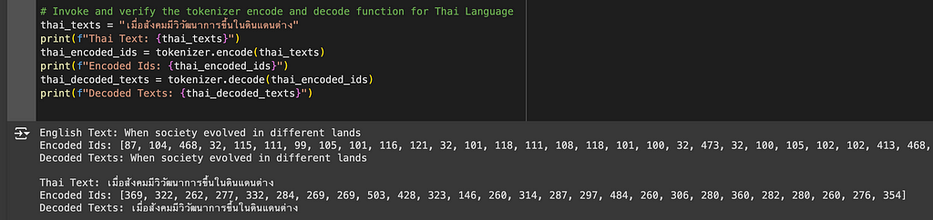
Perfect. Our Thai Tokenizer can now successfully and accurately encode and decode texts in both Thai and English languages.
Have you noticed that the encoded IDs for English texts are longer than Thai encoded IDs? This is because we’ve only trained our tokenizer with the Thai dataset. Hence the tokenizer is only able to build a comprehensive vocabulary for the Thai language. Since we didn’t train with an English dataset, the tokenizer has to encode right from the character level which results in longer encoded IDs. As I have mentioned before, for multilingual LLM, you should train both the English and Thai datasets with a ratio of 2:1. This will give you balanced and quality results.
And that is it! We have now successfully created our own Thai Tokenizer from scratch only using Python. And, I think that was pretty cool. With this, you can easily build a tokenizer for any foreign language. This will give you a lot of leverage while implementing your Multilingual LLM.
Thanks a lot for reading!
References
[1] Andrej Karpathy, Git Hub: Karpthy/minbpe
Build a Tokenizer for the Thai Language from Scratch was originally published in Towards Data Science on Medium, where people are continuing the conversation by highlighting and responding to this story.
Originally appeared here:
Build a Tokenizer for the Thai Language from Scratch
Go Here to Read this Fast! Build a Tokenizer for the Thai Language from Scratch