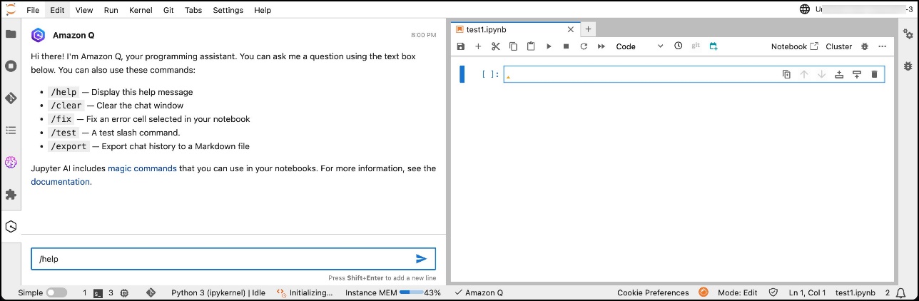
In this post, we present a real-world use case analyzing the Diabetes 130-US hospitals dataset to develop an ML model that predicts the likelihood of readmission after discharge.
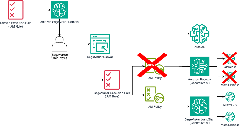
In this post, we analyze strategies for governing access to Amazon Bedrock and SageMaker JumpStart models from within SageMaker Canvas using AWS Identity and Access Management (IAM) policies. You’ll learn how to create granular permissions to control the invocation of ready-to-use Amazon Bedrock models and prevent the provisioning of SageMaker endpoints with specified SageMaker JumpStart models.
This post offers insights for businesses aiming to use artificial intelligence (AI) and cloud technologies to enhance customer service and streamline operations. We share how Rocket Mortgage’s use of AWS services set a new industry standard and demonstrate how to apply these principles to transform your client interactions and processes.
What I learned doing semantic search on U.S. Presidents with four language model embeddings
All photos in this article are from WikiCommons and are either public domain or licensed for commercial use.
I’m interested in trying to figure out what’s inside a language model embedding. You should be too, if one if these applies to you:
· The “thought processes” of large language models (LLMs) intrigues you.
· You build data-driven LLM systems, (especially Retrieval Augmented Generation systems) or would like to.
· You plan to use LLMs in the future for research (formal or informal).
· The idea of a brand new type of language representation intrigues you.
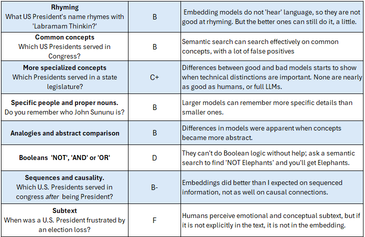
This blog post is intended to be understandable to any curious person, but even if you are language model specialist who works with them daily I think you will learn some useful things, as I did. Here’s a scorecard summary of what I learned about Language Model embeddings by performing semantic searches with them:
The Scorecard
What do embeddings “see” well enough to find passages in a larger dataset?
Along with many people, I have been fascinated by recent progress trying to look inside the ‘Black Box’ of large language models. There have recently been some incredible breakthroughs in understanding the inner workings of language models. Here are examples of this work by Anthropic, Google, and a nice review (Rai et al. 2024).
This exploration has similar goals, but we are studying embeddings, not full language models, and restricted to ‘black box’ inference from question responses, which is probably still the single best interpretability method.
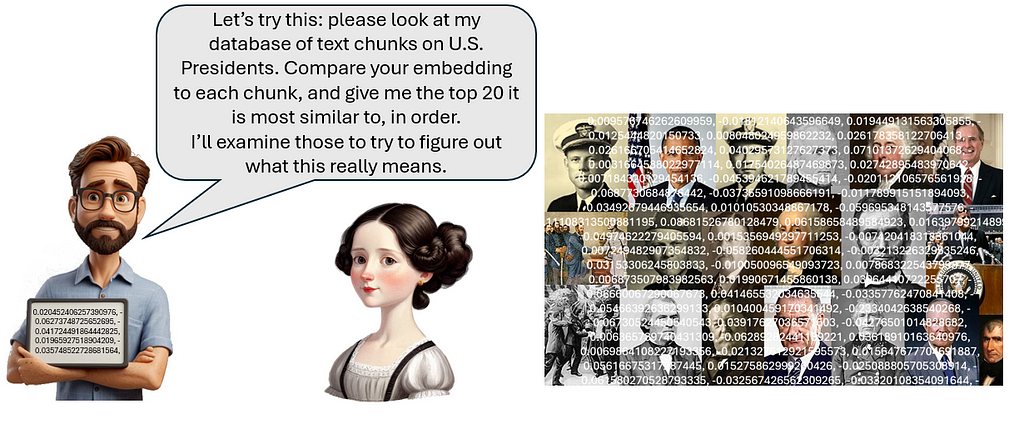
Embeddings are what are created by LLMs in the first step, when they take a chunk of text and turn it into a long string of numbers that the language model networks can understand and use. Embeddings are used in Retrieval Augmented Generation (RAG) systems to allow searching on semantics (meanings) than are deeper than keyword-only searches. A set of texts, in my case the Wikipedia entries on U.S. Presidents, is broken into small chunks of text and converted to these numerical embeddings, then saved in a database. When a user asks a question, that question is also converted to embeddings. The RAG system then searches the database for an embedding similar to the user query, using a simple mathematical comparison between vectors, usually a cosine similarity. This is the ‘retrieval’ step, and the example code I provide ends there. In a full RAG system, whichever most-similar text chunks are retrieved from the database are then given to an LLM to use them as ‘context’ for answering the original question.
If you work with RAGs, you know there are many design variants of this basic process. One of the design choices is choosing a specific embedding model among the many available. Some models are longer, trained on more data, and cost more money, but without an understanding of what they are like and how they differ, the choice of which to use is often guesswork. How much do they differ, really?
If you don’t care about the RAG part
If you do not care about RAG systems but are just interested in learning more conceptually about how language models work, you might skip to the questions. Here is the upshot: embeddings encapsulate interesting data, information, knowledge, and maybe even wisdom gleaned from text, but neither their designers nor users knows exactly what they capture and what they miss. This post will search for information with different embeddings to try to understand what is inside them, and what is not.
The technical details: data, embeddings and chunk size
The dataset I’m using contains Wikipedia entries about U.S. Presidents. I use LlamaIndex for creating and searching a vector database of these text entries. I used a smaller than usual chunk size, 128 tokens, because larger chunks tend to overlay more content and I wanted a clean test of the system’s ability to find semantic matches. (I also tested chunk size 512 and results on most tests were similar.)
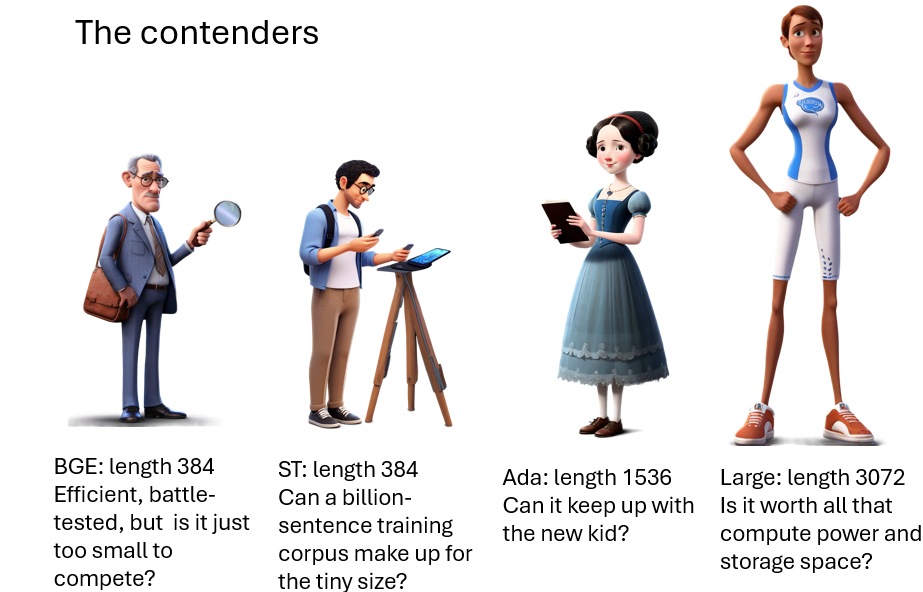
I’ll tests four embeddings:
1. BGE (bge-small-en-v1.5) is quite small at length 384. It the smallest of a line of BGE’s developed by the Beijing Academy of Artificial Intelligence. For it’s size, it does well on benchmark tests of retrieval (see leaderboard). It is F=free to use from HuggingFace.
2. ST (all-MiniLM-L6-v2) is another 384-length embedding. It excels at sentence comparisons; I’ve used it before for judging transcription accuracy. It was trained on the first billion sentence-pair corpus, which was about half Reddit data. It is also available HuggingFace.
Graphics by the author, using Leonardo.ai
3. Ada (text-embedding-ada-002) is the embedding scheme that OpenAI used from GPT-2 through GPT-4. It is much longer than the other embeddings at length 1536, but it is also older. How well can it compete with newer models?
4. Large (text-embedding-3-large) is Ada’s replacement — newer, longer, trained on more data, more expensive. We’ll use it with the max length of 3,072. Is it worth the extra cost and computing power? Let’s find out.
Questions, code available on GitHub
There is spreadsheet of question responses, a Jupyter notebook, and text dataset of Presidential Wikipedia entries available here:
Download the text and Jupyter notebook if you want to build your own; mine runs well on Google Colab.
The Spreadsheet of questions
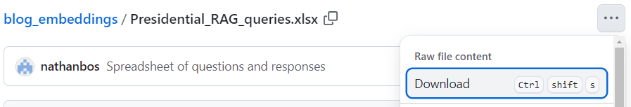
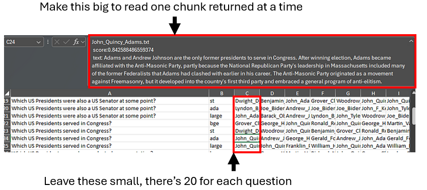
I recommend downloading the spreadsheet to understand these results. It shows the top 20 text chunks returned for each question, plus a number of variants and follow-ups. Follow the link and choose ‘Download’ like this:
Screenshot by the author
To browse the questions and responses, I find it easiest to drag the text entry cell at the top larger, and tab through the responses to read the text chunks there, as in this screenshot.
Screenshot by the author
Not that this is the retrieved context only, there is no LLM synthesized response to these questions. The code has instructions for how to get those, using a query engine instead of just a retriever as I did.
Providing understanding that goes beyond leaderboards
We’re going to do something countercultural in this post: we’re going to focus on the actual results of individual question responses. This stands in contrast to current trends in LLM evaluation, which are about using larger and larger datasets and and presenting results aggregated to a higher and higher level. Corpus size matters a lot for training, but that is not as true for evaluation, especially if the goal is human understanding.
For aggregated evaluation of embedding search performance, consult the (very well implemented) HuggingFace leaderboard using the (excellent) MTEB dataset: https://huggingface.co/spaces/mteb/leaderboard.
Leaderboards are great for comparing performance broadly, but are not great for developing useful understanding. Most leaderboards do not publish actual question-by-question results, limiting what can be understood about those results. (They do usually provide code to re-run the tests yourself.) Leaderboards also tend to focus on tests that are roughly within the current technology’s abilities, which is reasonable if the goal is to compare current models, but does not help understand the limits of the state of the art. To develop usable understanding about what systems can and cannot do, I find there is no substitute for back-and-forth testing and close analysis of results.
What I’m presenting here is basically a pilot study. The next step would be to do the work of developing larger, precisely designed, understanding-focused test sets, then conduct iterative tests focused on deeper understanding of performance. This kind of study will likely only happen at scale when funding agencies and academic disciplines beyond computer science start caring about LLM interpretability. In the meantime, you can learn a lot just by asking.
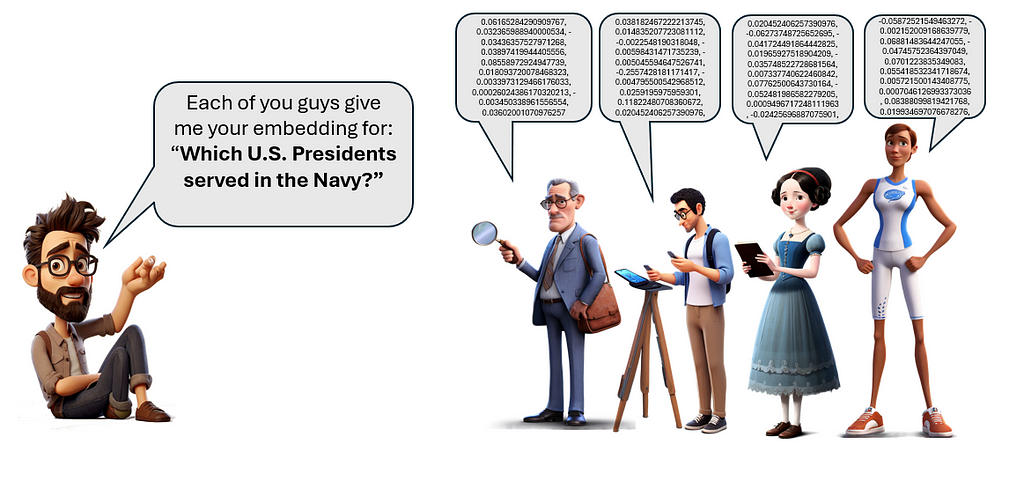
Question: Which U.S. Presidents served in the Navy?
Let’s use the first question in my test set to illustrate the ‘black box’ method of using search to aid understanding.
graphics by the author, using Leonardo.aiGraphics by the author, using Leonardo.aiAnimated graphics by the author, using Leonardo.ai. Presidential portraits from WikiCommons, public domain or commercial license.
The results:
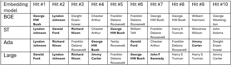
I gave the Navy question to each embedding index (database). Only one of the four embeddings, Large, was able to find all six Presidents who served in the Navy within the top ten hits. The table below shows the top 10 found passages from for each embedding model. See the spreadsheet for full text of the top 20. There are duplicate Presidents on the list, because each Wikipedia entry has been divided into many individual chunks, and any given search may find more than one from the same President.
Why were there so many incorrect hits? Let’s look at a few.
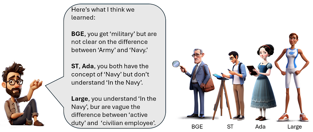
The first false hit from BGE is a chunk from Dwight D Eisenhower, an army general in WW2, that has a lot of military content but has nothing to do with the Navy. It appears that BGE does have some kind of semantic representation of ‘Navy’. BGE’s search was better than what you would get with a simple keyword matches on ‘Navy’, because it generalizes to other words that mean something similar. But it generalized too indiscriminately, and failed to differentiate Navy from general military topics, e.g. it does not consistently distinguish between the Navy and the Army. My friends in Annapolis would not be happy.
How did the two mid-level embedding models do? They seem to be clear on the Navy concept and can distinguish between the Navy and Army. But they each had many false hits on general naval topics; a section on Chester A Arthur’s naval modernization efforts shows up high on both lists. Other found sections have Presidential actions related to the Navy, or ships named after Presidents, like the U.S.S. Harry Truman.
The middle two embedding models seem to have a way to semantically represent ‘Navy’ but do not have a clear semantic representation of the concept ‘Served in the Navy’. This was enough to prevent either ST or Ada from finding all six Naval-serving Presidents in the top ten.
On this question, Large clearly outperforms the others, with six of the seven top hits corresponding to the six serving Presidents: Gerald Ford, Richard Nixon, Lyndon B. Johnson, Jimmy Carter, John F. Kennedy, and George H. W. Bush. Large appears to understand not just ‘Navy’ but ‘served in the Navy’.
What did Large get wrong?
What was the one mistake in Large? It was the chunk on Franklin Delano Roosevelt’s work as Assistant Secretary of the Navy. In this capacity, he was working for the Navy, but as a civilian employee, not in the Navy. I know from personal experience that the distinction between active duty and civilian employees can be confusing. The first time I did contract work for the military I was unclear on which of my colleagues were active duty versus civilian employees. A colleagues told me, in his very respectful military way, that this distinction was important, and I needed to get it straight, which I have since. (Another pro tip: don’t get the ranks confused.)
Question: Which U.S. Presidents worked as a civilian employees of the Navy?
In this question I probed to see whether the embeddings “understood” this distinction that I had at first missed: do they know how civilian employees of the Navy differs from people actually in the service? Both Roosevelts worked for the Navy in a civilian capacity. Theodore had also been in the Army (leading the charge of San Juan Hill), wrote books about the Navy, and built up the Navy as President, so there are many Navy-related chunks about TR, but he was never in the Navy. (Except as Commander in Chief; this role technically makes all Presidents part of the U.S. Navy, but that relationship did not affect search hits.)
The results of the civilian employee query can be seen in the results spreadsheet. The first hit for Large and second for Ada is a passage describing some of FDR’s work in the Navy, but this was partly luck because it included the word ‘civilian’ in a different context. Mentions were made of staff work by LBJ and Nixon, although it is clear from the passages that they were active duty at the time. (Some staff jobs can be filled by either military or civilian appointees.) Mention of Teddy Roosevelt’s civilian staff work did not show up at all, which would prevent an LLM from correctly answering the question based on these hits.
Overall there were only minor difference between the searches for Navy, “In the Navy” and “civilian employee”. Asking directly about active-duty Navy gave similar results. The larger embedding models had some correct associations, but overall could not make the necessary distinction well enough to answer the question.
graphics by the author, using Leonardo.ai
Common Concepts
Question: Which U.S. Presidents were U.S. Senators before they were President?
All of the vectors seem to generally understand common concepts like this, and can give good results that an LLM could turn into an accurate response. The embeddings could also differentiate between the U.S. Senate and U.S. House of Representatives. They were clear on the difference between Vice President and President, the difference between a lawyer and a judge, and the general concept of an elected representative.
They also all did well when asked about Presidents who were artists, musicians, or poker players. They struggled a little with ‘author’ because there were so many false positives in the data relate to other authors.
More Specialized Concepts
As we saw, they each have their representational limits, which for Large was the concept of ‘civilian employee of the Navy.’ They also all did poorly on the distinction between national and state representatives.
Question: Which U.S. President served as elected representatives at the state level?
None of the models returned all, or even most of the Presidents who served in state legislatures. All of the models mostly returned hits relate to the U.S. House of Representatives, with some references to states or governors. Large’s first hit was on target: “Polk was elected to its state legislature in 1823”, but missed the rest. This topic could use some more probing, but in general this concept was a fail.
Question: Which US Presidents were not born in a US State?
All four embeddings returned Barack Obama as one of the top hits to this question. This is not factual — Hawaii was a state in 1961 when Obama was born there, but the misinformation is prevalent enough (thanks, Donald) to show up in the encoding. The Presidents who were born outside of the United States were the early ones, e.g. George Washington, because Virginia was not a state when he was born. This implied fact was not accessible via the embeddings. William Henry Harrison was returned in all cases, because his entry includes the passage “…he became the last United States president not born as an American citizen”, but none of the earlier President entries said this directly, so it was not found in the searches.
Search for specific, semi-famous people and places
Question: Which U.S. Presidents were asked to deliver a difficult message to John Sununu?
John Sununu, From WikiCommons. Photo by Michael Vadon
People who are old enough to have followed U.S. politics in the 1990s will remember this distinctive name: John Sununu was governor of New Hampshire, was a somewhat prominent political figure, and served as George H.W. Bush’s (Bush #1’s) chief of staff. But he isn’t mentioned in Bush #1’s entry. He is mentioned in a quirky offhand anecdote in the entry for George W. Bush (Bush #2) where Bush #1 asked Bush #2 to ask Sununu to resign. This was mentioned, I think, to illustrate one of Bush #2’s key strengths, likability, and the relationship between the two Bushes. A search for John Sununu, which would have been easy for a keyword search due to the unique name, fails to find this passage in three of the four embeddings. The one winner? Surprisingly, it is BGE, the underdog.
There was another interesting pattern: Large returned a number of hits on Bush #1, the President historically most associated with Sununu, even though he is never mentioned in the returned passages. This seems more than a coincidence; the embedding encoded some kind of association between Sununu and Bush #1 beyond what is stated in the text.
Which U.S. Presidents were criticized by Helen Prejean?
Sister Helen Prejean, from WikiCommons. Photo by Don LaVange
I observed the same thing with a second semi-famous name: Sister Helen Prejean was a moderately well-known critic of the death penalty; she wrote Dead Man Walking and Wikipedia briefly notes that she criticized Bush #2’s policies. None of the embeddings were able to find the Helen Prejean mention which, again, a keyword search would have found easily. Several of Large’s top hits are passages related to the death penalty, which seems like more than a coincidence. As with Sununu, Large appears to have some association with the name, even though it is not represented clearly enough in the embedding vocabulary to do an effective search for it.
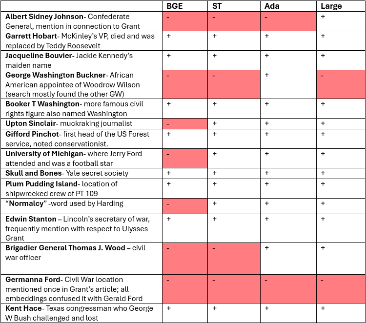
I tested a number of other specific names, places, and one weird word, ‘normalcy’, for the embedding models’ ability to encode and match them in the Wikipedia texts. The table below shows the hits and misses.
Screenshot by the author
What does this tell us?
Language models encode more frequently-encountered names, i.e. more famous people, but are less likely to encode them the more infrequent they are. Larger embeddings, in general, encode more specific details. But there were cases here smaller models outperformed larger ones, and models also sometimes had to have some associations even with name that they cannot recognize well enough to find. A great follow up on this would be a more systematic study of how noun frequency affects representation in embeddings.
Tangent #1: Rhyming
This was a bit of a tangent but I had fun testing it. Large Language models cannot rhyme very well, because they neither speak or hear. Most humans learn to read aloud first, and learn to read silently only later. When we read silently, we can still subvocalize the words and ‘hear’ the rhymes in written verse as well. Language models do not do this. Theirs is a silent, text-only world. They know about rhyming only from reading about it, and never get very good at it. Embeddings could theoretically represent phonetics, and can usually give accurate phonetics for a given word. But I’ve been testing rhyming on and off since GPT-3, and LLMs usually can’t search on this. However, the embeddings surprised me a few times in this exercise.
Which President’s name rhymes with ‘Gimme Barter?’
This one turned out to be easy; all four vectors gave “Jimmy Carter” as the first returned hit. The cosine similarities were lowish, but since this was essentially a multiple choice test of Presidents, they all made the match easily. I think the spellings of Gimme Barter and Jimmy Carter are too similar, so let’s try some harder ones, with more carefully disguised rhymes that sound alike but have dissimilar spellings.
Which US President’s name rhymes with Laybramam Thinkin’?
From WikiCommons: photo of Abraham Lincoln, by Alexander Gardner.
This one was harder. Abraham Lincoln did not show up on BGE or ST’s top ten hits, but was #1 for Ada and #3 for Large.
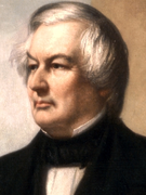
Which US President’s names rhymes with Will-Ard Syl-Bor?
Millard Fillmore was a tough rhyme. It was #2 for Ada, #5 for Large, not in the top 10 for the others. The lack of Internet poetry about President Fillmore seems like a gap someone needs to fill. There were a lot of false hits for Bill Clinton, perhaps because of the double L’s?
Google search results obtained by author; Portrait of Millard Fillmore by George Peter Alexander Healey from WikiCommons
Which US President’s name rhymes with Mayrolled Gored?
Gerald Ford was #7 for BGE , #4 for Ada, #5 for Large.
Rhyming was not covered at the Gerald R. Ford Presidential Museum in my hometown of Grand Rapids, Michigan. I would know, I visited it many times. More on that later.
Takeaway: the larger embedding schemes can rhyme, a little, although maybe less well than a human. How are they doing this, and what are the limits? Are they analyzing phonetics, taking advantage of existing rhyming content, or making good guesses another way? I have no idea. Phonetic encoding in embedding systems seems like a fine thesis topic for some enterprising linguistics student, or maybe a very nerdy English Lit major.
Embedding can’t do Booleans: no NOT, AND, or OR
Simple semantic search cannot do some basic operations the keyword query systems generally can, and are not good at searching for sequences of events.
Question: Which Presidents were NOT Vice President first?
Doing a vector search with ‘NOT’ is similar to the old adage about telling someone not to think about a Pink Elephant — saying the phrase usually causes the person to do so. Embeddings have no representation of ‘Not Vice President’, they only have Vice President.
Image by the author, using GPT-4o (Dall-E)
The vector representing the question will contain both “President” and “Vice President” and tend to find chunks with both. One could try to kludge a compound query, searching first for all President, then all Vice Presidents, and subtract, but the limit on contexts returned would prevent returning all of the first list, and is not guaranteed to get all of the second. Boolean search with embeddings remains a problem.
Question: Which U.S. President was NOT elected as vice President and NEVER elected as President?
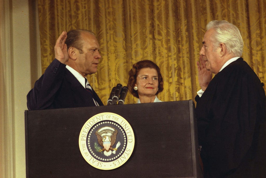
An exception the the ‘NOT’ fail: all of the embeddings could find the passage saying that Gerald Ford was the only President that was never elected to be Vice President (appointed when Spiro Agnew resigned) or President (took Nixon’s place when he resigned, lost the re-election race to Jimmy Carter.) They were able to find this because the ‘not’ was explicitly represented in the text, with no inference needed, and it is also a well-known fact about Ford.
Why is there a double negative in this question?
The unnecessary double negative in the prior question made this search better. A search on “Which U.S. President was not elected as either Vice President or President?” gave poorer results. I added the double negative wording as a hunch that the double negatives would have a compound effect of making the query more both negative and make it easier to connect the ‘not’ to both offices. This does not make grammatical sense but does make sense in the world of superimposed semantics.
Gerald R. Ford’s many accomplishments
People who have visited the Gerald R. Ford Presidential museum in my hometown of Grand Rapids, Michigan, a sufficient number of times will be aware that Ford made many important contributions despite not being elected to the highest offices. Just putting that out there.
Gerald Ford’s inauguration. From WikiCommons; public domain photo by Robert LeRoy Knudsen
Question: Which Presidents were President AND Vice President?
Semantic search has a sort of weak AND, more like an OR, but neither is a logical Boolean query. Embeddings do not link concepts with strict logic. Instead, think of them as superimposing concepts on top of each other on the same vector. This query would find chunks that load strongly on President (which is most of them in this dataset) and Vice President, but does not enforce the logical AND in any way. In this dataset it gives some correct hits, and a lot of extraneous mentions of Vice Presidents. This search for superimposed concepts is not a true logical OR either.
Embeddings and sequences of actions
Do embeddings connect concepts sequentially well enough to search on these sequences? My going-in assumption was that they cannot, but the embeddings did better than expected.
Humans have a specific types of memory for sequence, called episodic memory. Stories are an important type of information for us; we encode things like personal history, social information and also useful lessons as stories. We can also recognize stories similar to ones that we already know. We can read a story about a hero who fails because of his fatal flaw, or an ordinary person who rises to great heights, and recognize not just the concepts but the sequence of actions. In my previous blog post on RAG search using Aesop’s Fables, the RAG system did not seem to have any ability to search on sequences of actions. I expected a similar failure here, but the results were a little different.
Question: Which US Presidents served in Congress after being President?
There were many Presidents who served in congress before being President, but only two who served in congress after being President. All of the Embeddings returned a passage from John Quincy Adams, which directly gives the answer, as a top hit: Adams and Andrew Johnson are the only former presidents to serve in Congress. All of them also separately found entries for Andrew Johnson in the top 10. There were a number of false hits, but the critical information was there.
The embeddings did not do as well on the follow-ups, like Which US Presidents served as judges after being President? But all did find mention of Taft, who notably was the only person to serve as chief justice and president.
Does this really represent successfully searching on a sequence? Possibly not; in these cases the sequence may be encapsulated in a single searchable concept, like “former President”. I still suspect that embeddings would badly underperform humans on more difficult story-based searches. But this is a subtle point that would require more analysis.
What about causal connections?
Causal reasoning is such an important part of human reasoning that I wanted to separately test whether causal linkages are clearly represented and searchable. I tested these with two paired queries that had the causality reversed, and looked both at which search hits were returned, and how the pairs different. Both question pairs were quite interesting and results are shown in the spreadsheet; I will focus on this one:
Question: When did a President’s action cause an important world event? -vs- When did an important world event cause a President’s action?
ST failed this test, it returned exactly the same hits in the same order for both queries. The causal connection was not represented clearly enough to affect the search.
All of the embeddings returned multiple chunks related to Presidential world travel, weirdly failing to separate traveling from official actions.
None of the embeddings did well on the causal reversal. Every one had hits where world events coincided with Presidential actions, often very minor actions, with no causal link in either direction. There all had false hits where the logical linkage went in the wrong directions (Presidents causing events vs responding to events). There were multiple example of commentators calling out Presidential inaction, which suggests that ‘act’ and ‘not act’ are conflated. Causal language, especially the word ‘cause’ triggered a lot of matches, even when it was not attached to a Presidential action or world event.
A deeper exploration of how embeddings represent causality, maybe in a critical domain like medicine, would be in order. What I observed is a lack of evidence that embeddings represent and correctly use causality.
Analogies
Question: Which U.S. Presidents were similar to Simon Bolivar, and how?
Simon Bolivar, revolutionary leader and later political leader in South America, is sometimes called the “George Washington of South America”. Could the embedding models perceive this analogy in the other direction?
BGE- Gave a very weird set of returned context, with no obvious connection besides some mentions of Central/ South American.
ST- Found a passage about William Henry Harrison’s 1828 trip to Colombia and feuding with Bolivar, and other mentions of Latin America, but made no abstract matches.
Ada- Found the Harrison passage + South America references, but no abstract matches that I can tell.
Large- Returned George Washington as hit #5 behind Bolivar/ S America hits.
Large won this test in a landslide. This hit shows the clearest pattern of larger/better vectors outperforming others at abstract comparisons.
Images in public domain, obtain from Wiki commons. Statue of Simon Bolivar by Emmanuel Frémiet, photo by Jebulon. Washington Crossing the Delaware painting by Emmanuel Leutze.
Abstract concepts
I tested a number of searches on more abstract concepts. Here are two examples:
Questions: Which US Presidents exceeded their power?
BGE: top hit: “In surveys of U.S. scholars ranking presidents conducted since 1948, the top three presidents are generally Lincoln, Washington, and Franklin Delano Roosevelt, although the order varies.” BGE found hits all related to Presidential noteworthiness, especially rankings by historians, I think keying on the words ‘power’ and ‘exceed’. This was a miss.
ST: “Roosevelt is widely considered to be one of the most important figures in the history of the United States.” Same patterns as BGE; a miss.
Ada: Ada’s hits were all on the topic of Presidential power, not just prestige, and so were more on-target than the smaller models. There is a common theme of increasing power, and some passages that imply exceeding, like this one: the Patriot Act “increased authority of the executive branch at the expense of judicial opinion…” Overall, not a clear win, but closer.
Large: It did not find the best 10 passages, but the hits were more on target. All had the concept of increasing Presidential power, and most has a flavor of exceeding some previous limit, e.g. “conservative columnist George Will wrote in The Washington Post that Theodore Roosevelt and Wilson were the “progenitors of today’s imperial presidency”
Again, there was a pattern of larger models having more precise, on-target abstractions. Large was the only one to get close to a correct representation of a President “exceeding their power” but even this performance left a lot of room for improvement.
Embeddings do not understand subtext
Subtext is meaning in a text that is not directly stated. People add meaning to what they read, making emotional associations, or recognizing related concepts that go beyond what is directly stated, but embeddings do this only in a very limited way.
Question: Give an example of a time when a U.S. President expressed frustration with losing an election?
In 1960, then-Vice President Richard Nixon lost a historically close election to John F Kennedy. Deeply hurt by the loss, Nixon decided to settle to return home to his home state of California and ran for governor in 1962. Nixon lost that race too. He famously announced at a press conference, “You don’t (won’t) have Nixon to kick around anymore because, gentlemen, this is my last press conference,” thus ending his political career, or so everyone thought.
Graphic by the author and GPT4o( Dall-E). There is no intentional resemblance with specific Presidents; these are Dall-E’s ideas about generic Presidential-looking men expressing emotions. Not bad.
What happens when you search for: “Give an example of a time when a U.S. President expressed frustration with losing an election”? None of the embeddings return this Nixon quote. Why? Because Wikipedia never directly states that he was frustrated, or had any other specific emotion; that is all subtext. When a mature human reads “You won’t have Nixon to kick around anymore”, we recognize some implied emotions, probably without consciously trying to do so. This might be so automatic when reading that one thinks it is in the text. But in his passage the emotion is never directly stated. And if it is subtext, not text, an embedding will (probably) not be able to represent it or be able to search it.
Wikipedia avoids speculating on emotional subtext as a part of fact-based reporting. Using subtext instead of text is also considered good tradecraft for fiction writers, even when the goal is to convey strong emotions. A common piece of advice for new writers is, “show, don’t tell.” Skilled writers reveal what characters are thinking and feeling without directly stating it. There’s even a name for pedantic writing that explains things too directly, it is called “on-the-nose dialogue”.
But “show, don’t tell” makes some content invisible to embeddings, and thus to vector-based RAG retrieval systems. This presents some fundamental barriers to what can be found in RAG system in the domain of emotional subtext, but also other layers of meaning that go beyond what is directly stated. I also did a lot of probing around concepts like Presidential mistakes, Presidential intentions, and analytic patterns that are just beyond what is directly stated in the text. Embedding-based search generally failed on this, mostly returning only direct statements, even when they were not relevant.
Why are embeddings shallow compared to Large Language Models?
Large Language Models like Claude and GPT-4 have the ability to understand subtext; they do a credible job explaining stories, jokes, poetry and Taylor Swift song lyrics. So why can’t embeddings do this?
Language models are comprised of layers, and in general the lower layers are shallower forms of processing, representing aspects like grammar and surface meanings, while higher level of abstraction occur in higher layers. Embeddings are the first stage in language model processing; they convert text into numbers and then let the LLM take over. This is the best explanation I know of for why the embedding search tests seem to plateau at shallower levels of semantic matching.
Embedding were not originally designed for RAGs; using them for semantic search is a clever, but ultimately limited secondary usage. That is changing, as embedding systems are being optimized for search. BGE was to some extend optimized for search, and ST was designed for sentence comparison; I would say this is why both BGE and ST were not too far behind Ada and Large despite being a fraction of the size. Large was probably designed with search in mind to a limited extent. But it was easy to push each of them to their semantic limits, as compared with the kind of semantics processed by full large language models.
Conclusion
What did we learn, conceptually, about embeddings in his exercise?
The embedding models, overall, surprised me on a few things. The semantic depth was less than I expected, based on the performance of the language models that use them. But they outperformed my expectations on a few things I expected them to fail completely at, like rhyming and searching for sequenced activities. This activity piqued my interest in probing some more specific areas; perhaps it did for you as well.
For RAG developers, this illuminated some of the specific ways that larger models may outperform smaller ones, including the precisions of their representation, the breadth of knowledge and the range of abstractions. As a sometime RAG builder, I have been skeptical that paying more for embeddings would lead to better performance, but this exercise convinced me that embedding choice can make a difference for some applications.
Embeddings systems will continue to incrementally improve, but I think some fundamental breakthroughs will be needed in this area. There is some current research on innovations like universal text embeddings.
Knowledge graphs are a popular current way to supplement semantic search. Graphs are good for making cross-document connections, but the LLM-derived graphs I have seen are semantically quite shallow. To get semantic depth from a knowledge graph probably requires a professionally-developed ontology to be available to serve as a starting point; these are available for some specialized fields.
My own preferred method is to improve text with more text. Since full language models can perceive and understand meaning that is not in embeddings, why not have a language model pre-process and annotate the text in your corpus with the specific types of semantics you are interested in? This might be too expensive for truly huge datasets, but for data in the small to medium range it can be an excellent solution.
I experimented with adding annotations to the Presidential dataset. To make emotional subtext searchable I had GPT4o write narratives for each President highlighting the personal and emotional content. These annotations were added back into the corpus. They are not great prose, but the concept worked. GPT’s annotation of the Nixon entry included the sentence: “The defeat was a bitter pill to swallow, compounded by his loss in the 1962 California gubernatorial race. In a moment of frustration, Nixon declared to the press, ‘You won’t have Nixon to kick around anymore,’ signaling what many believed to be the end of his political career”. This effectively turned subtext into text, making is searchable.
I experimented with a number of types of annotations. One that I was particularly happy used Claude to examine each Presidency and make comments on underlying system dynamical phenomena like delayed feedback and positive feedback loops. Searching on these terms on the original text gave nothing useful, but greatly improved with annotations. Claude’s analyses were not brilliant, or even always correct, but it found and annotated enough decent examples that searches using system dynamic language found useful content.
The Gerald R Ford Presidential Museum in Grand Rapids, Michigan. Photo from WikiCommons, taken by museum staff.Oval office replica, the coolest thing in the Gerald R. Ford Presidential museum. Image from WikiCommons; photo by JJonahJackalope
And the difference between weak vs strong grounding
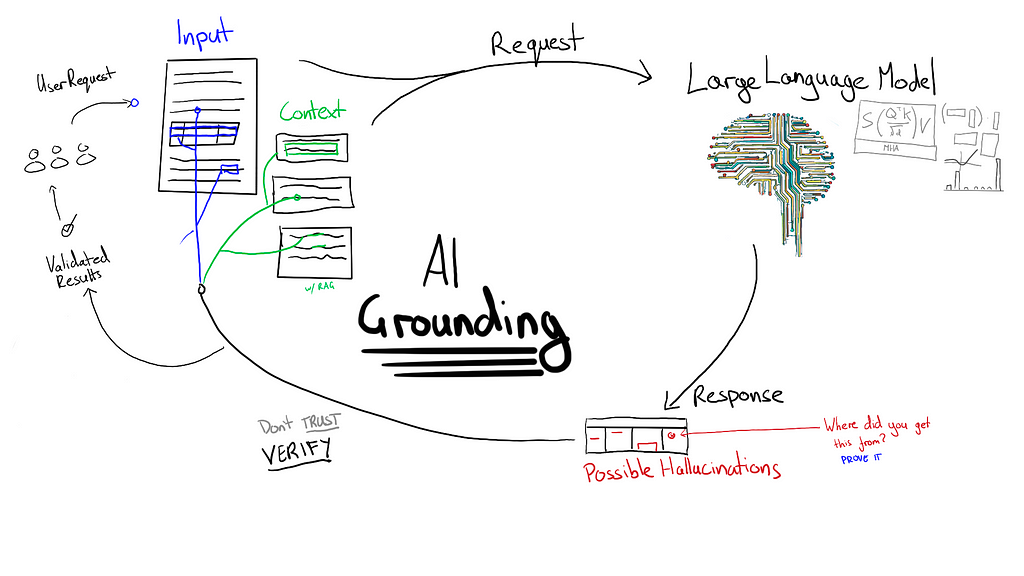
Image by the author
I work as an AI Engineer in a particular niche: document automation and information extraction. In my industry using Large Language Models has presented a number of challenges when it comes to hallucinations. Imagine an AI misreading an invoice amount as $100,000 instead of $1,000, leading to a 100x overpayment. When faced with such risks, preventing hallucinations becomes a critical aspect of building robust AI solutions. These are some of the key principles I focus on when designing solutions that may be prone to hallucinations.
Using validation rules and “human in the loop”
There are various ways to incorporate human oversight in AI systems. Sometimes, extracted information is always presented to a human for review. For instance, a parsed resume might be shown to a user before submission to an Applicant Tracking System (ATS). More often, the extracted information is automatically added to a system and only flagged for human review if potential issues arise.
A crucial part of any AI platform is determining when to include human oversight. This often involves different types of validation rules:
1. Simple rules, such as ensuring line-item totals match the invoice total.
2. Lookups and integrations, like validating the total amount against a purchase order in an accounting system or verifying payment details against a supplier’s previous records.
An example validation error when there needs to be a human in the loop. Source: Affinda
These processes are a good thing. But we also don’t want an AI that constantly triggers safeguards and forces manual human intervention. Hallucinations can defeat the purpose of using AI if it’s constantly triggering these safeguards.
Small Language Models
One solution to preventing hallucinations is to use Small Language Models (SLMs) which are “extractive”. This means that the model labels parts of the document and we collect these labels into structured outputs. I recommend trying to use a SLMs where possible rather than defaulting to LLMs for every problem. For example, in resume parsing for job boards, waiting 30+ seconds for an LLM to process a resume is often unacceptable. For this use case we’ve found an SLM can provide results in 2–3 seconds with higher accuracy than larger models like GPT-4o.
An example from our pipeline
In our startup a document can be processed by up to 7 different models — only 2 of which might be an LLM. That’s because an LLM isn’t always the best tool for the job. Some steps such as Retrieval Augmented Generation rely on a small multimodal model to create useful embeddings for retrieval. The first step — detecting whether something is even a document — uses a small and super-fast model that achieves 99.9% accuracy. It’s vital to break a problem down into small chunks and then work out which parts LLMs are best suited for. This way, you reduce the chances of hallucinations occurring.
Distinguishing Hallucinations from Mistakes
I make a point to differentiate between hallucinations (the model inventing information) and mistakes (the model misinterpreting existing information). For instance, selecting the wrong dollar amount as a receipt total is a mistake, while generating a non-existent amount is a hallucination. Extractive models can only make mistakes, while generative models can make both mistakes and hallucinations.
Risk tolerance and Grounding
When using generative models we need some way of eliminating hallucinations.
Grounding refers to any technique which forces a generative AI model to justify its outputs with reference to some authoritative information. How grounding is managed is a matter of risk tolerance for each project.
For example — a company with a general-purpose inbox might look to identify action items. Usually, emails requiring actions are sent directly to account managers. A general inbox that’s full of invoices, spam, and simple replies (“thanks”, “OK”, etc.) has far too many messages for humans to check. What happens when actions are mistakenly sent to this general inbox? Actions regularly get missed. If a model makes mistakes but is generally accurate it’s already doing better than doing nothing. In this case the tolerance for mistakes/hallucinations can be high.
Other situations might warrant particularly low risk tolerance — think financial documents and “straight-through processing”. This is where extracted information is automatically added to a system without review by a human. For example, a company might not allow invoices to be automatically added to an accounting system unless (1) the payment amount exactly matches the amount in the purchase order, and (2) the payment method matches the previous payment method of the supplier.
Even when risks are low, I still err on the side of caution. Whenever I’m focused on information extraction I follow a simple rule:
If text is extracted from a document, then it must exactly match text found in the document.
This is tricky when the information is structured (e.g. a table) — especially because PDFs don’t carry any information about the order of words on a page. For example, a description of a line-item might split across multiple lines so the aim is to draw a coherent box around the extracted text regardless of the left-to-right order of the words (or right-to-left in some languages).
Forcing the model to point to exact text in a document is “strong grounding”. Strong grounding isn’t limited to information extraction. E.g. customer service chat-bots might be required to quote (verbatim) from standardised responses in an internal knowledge base. This isn’t always ideal given that standardised responses might not actually be able to answer a customer’s question.
Another tricky situation is when information needs to be inferred from context. For example, a medical assistant AI might infer the presence of a condition based on its symptoms without the medical condition being expressly stated. Identifying where those symptoms were mentioned would be a form of “weak grounding”. The justification for a response must exist in the context but the exact output can only be synthesised from the supplied information. A further grounding step could be to force the model to lookup the medical condition and justify that those symptoms are relevant. This may still need weak grounding because symptoms can often be expressed in many ways.
Grounding for complex problems
Using AI to solve increasingly complex problems can make it difficult to use grounding. For example, how do you ground outputs if a model is required to perform “reasoning” or to infer information from context? Here are some considerations for adding grounding to complex problems:
Identify complex decisions which could be broken down into a set of rules. Rather than having the model generate an answer to the final decision have it generate the components of that decision. Then use rules to display the result. (Caveat — this can sometimes make hallucinations worse. Asking the model multiple questions gives it multiple opportunities to hallucinate. Asking it one question could be better. But we’ve found current models are generally worse at complex multi-step reasoning.)
If something can be expressed in many ways (e.g. descriptions of symptoms), a first step could be to get the model to tag text and standardise it (usually referred to as “coding”). This might open opportunities for stronger grounding.
Set up “tools” for the model to call which constrain the output to a very specific structure. We don’t want to execute arbitrary code generated by an LLM. We want to create tools that the model can call and give restrictions for what’s in those tools.
Wherever possible, include grounding in tool use — e.g. by validating responses against the context before sending them to a downstream system.
Is there a way to validate the final output? If handcrafted rules are out of the question, could we craft a prompt for verification? (And follow the above rules for the verified model as well).
Key Takeaways
When it comes to information extraction, we don’t tolerate outputs not found in the original context.
We follow this up with verification steps that catch mistakes as well as hallucinations.
Anything we do beyond that is about risk assessment and risk minimisation.
Break complex problems down into smaller steps and identify if an LLM is even needed.
For complex problems use a systematic approach to identify verifiable task:
— Strong grounding forces LLMs to quote verbatim from trusted sources. It’s always preferred to use strong grounding.
— Weak grounding forces LLMs to reference trusted sources but allows synthesis and reasoning.
— Where a problem can be broken down into smaller tasks use strong grounding on tasks where possible.
Affinda AI Platform
We’ve built a powerful AI document processing platform used by organisations around the world.
The Real Odds of Encountering Alien Life (Part 5 of the Drake Equation Series)
Recap: Throughout this series, we’ve explored the factors that could lead to the existence of alien civilizations, starting from the number of habitable planets to the probability that intelligent civilizations have developed communication technology. In this final article, we approach the ultimate question: Have we ever encountered alien life? And will we ever encounter it in the future?
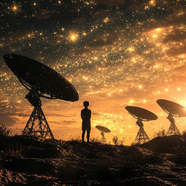
All images were developed by the author using Midjourney.
Step 10: A Rational Approach to Extraterrestrial Encounters
The search for extraterrestrial life has long been a mix of science, speculation, and sensationalism. From UFO sightings to government UAP (Unidentified Aerial Phenomena) reports, the public imagination has been captivated by the idea of alien encounters. But, from a scientific standpoint, how likely is it that we’ve already encountered alien life — or ever will?
This is where a rational, data-driven approach comes into play. Using a combination of the Drake Equation, modern simulations, and Bayesian probability models, we can finally calculate the likelihood of past and future encounters.
Why This Step Matters
It’s easy to get caught up in the excitement of potential alien encounters, but the reality is far more nuanced. Even if intelligent civilizations exist in the galaxy, the chances of them overlapping with our civilization in time and proximity are incredibly small. This step will help quantify the likelihood of these encounters based on both past and future possibilities, giving us a clearer picture of the odds we’re facing.
Bayesian Probability and Alien Encounters
Bayesian reasoning allows us to update our probability estimates as new evidence (or lack thereof) emerges. In the case of alien encounters, we can use this approach to assess the probabilities of both past and future contact.
Let’s break down the Bayesian approach:
P(H|E): The probability that aliens exist and we’ve encountered them given the current evidence.
P(H): Our prior probability, or the initial assumption of how likely it is that alien encounters have occurred or will occur.
P(E|H): The likelihood of the current evidence (e.g., no confirmed alien contact) assuming the hypothesis of an encounter is true.
P(E): The overall probability of the evidence, which accounts for all possible hypotheses.
We’ll use this framework to calculate both past and future encounters.
Bayesian Monte Carlo Simulation for Alien Encounters: Understanding the Approach
To quantify the probabilities of past and future alien encounters, we employed a Bayesian framework combined with Monte Carlo simulations to manage the inherent uncertainty in the parameters. This section walks you through the rationale and methodology behind these two approaches before presenting the actual code.
Why Use Bayesian Analysis?
Bayesian analysis is a robust method for updating the probability of an event based on new evidence. In our case, the event in question is whether we have encountered, or will encounter, alien civilizations. By incorporating both prior knowledge and the available (though limited) evidence — like the absence of confirmed contact — we can refine our estimates and quantify the uncertainty around past and future alien encounters.
Bayes’ theorem allows us to calculate the posterior probabilities — in other words, the likelihood of alien encounters given our assumptions and observations. This process is essential because it continuously updates our understanding as new information emerges, whether it’s confirmed evidence of extraterrestrial life or further lack of contact.
Why Monte Carlo Simulations?
Given the uncertainty and variability in the parameters of the Drake Equation and other likelihoods related to alien encounters, it would be unrealistic to use a single set of fixed values to estimate the probabilities. Instead, Monte Carlo simulations let us sample a broad range of plausible values for each parameter, such as the likelihood of contact or the prior probability that alien life exists.
By running thousands of simulations with these different values, we can explore a range of outcomes rather than relying on rigid point estimates. The result is a more nuanced understanding of how likely past and future encounters are, along with a clearer picture of the probability distributions for each scenario.
Now, let’s dive into the actual code implementation:
**********************************; **********************************; /* Set the random seed for reproducibility */ data _null_; call streaminit(1234); run;
/* Number of simulations */ %let num_simulations = 100000;
/* Number of civilizations to generate */ %let num_civilizations = 2364;
/* Galactic radius and height in light years */ %let galactic_radius = 50000; %let galactic_height = 1300;
/* Earth's position (assumed to be at 3/4 of the galactic radius) */ %let earth_position_x = &galactic_radius * 3 / 4; %let earth_position_y = 0; %let earth_position_z = 0;
/* Create a dataset to store civilization positions */ data civilization_positions; length Civilization $10.; input Civilization $ Position_X Position_Y Position_Z; datalines; Earth &earth_position_x &earth_position_y &earth_position_z ; run;
/* Generate random positions for other civilizations */ data civilization_positions; set civilization_positions; do i = 1 to &num_civilizations; Position_X = rand("Uniform") * &galactic_radius; Position_Y = rand("Uniform") * 2 * &galactic_height - &galactic_height; Position_Z = rand("Uniform") * 2 * &galactic_height - &galactic_height; Civilization = "Civilization " || strip(put(i, 8.)); output; end; drop i; run;
/* Calculate the distance between civilizations and Earth */ data civilization_distances; set civilization_positions; Distance = sqrt((Position_X - &earth_position_x)**2 + (Position_Y - &earth_position_y)**2 + (Position_Z - &earth_position_z)**2); run;
/* Calculate the minimum distance to Earth for each civilization */ proc sql; create table civilization_min_distance as select Civilization, Distance as Min_Distance from civilization_distances order by Distance; quit;
/* Calculate the probability of encountering civilizations based on distance */ data probability_encounter; set civilization_min_distance; Probability = 1 / (1 + Min_Distance); run;
/* Calculate the average probability for each distance band */ proc sql; create table average_probability as select case when Min_Distance <= 1000 then 'Close' when Min_Distance > 1000 and Min_Distance <= 3000 then 'Medium' when Min_Distance > 3000 then 'Far' end as Distance_Band, avg(Probability) as Average_Probability from probability_encounter group by case when Min_Distance <= 1000 then 'Close' when Min_Distance > 1000 and Min_Distance <= 3000 then 'Medium' when Min_Distance > 3000 then 'Far' end; quit;
/* Print the result */ proc print data=average_probability; run;
/* Select the closest civilization to Earth and its associated probability */ proc sql; create table closest_civilization as select Civilization, Min_Distance, Probability from probability_encounter where Min_Distance = (select min(Min_Distance) from probability_encounter); quit;
/* Print the result */ proc print data=closest_civilization; run;
/*Bayesian analysis for probability of encountering aliens in the past or future*/
/* Set seed for reproducibility */ %let num_iterations = 100;
/* Create Bayesian analysis dataset */ data bayesian_analysis; call streaminit(123);
/* Output the results */ do i = 1 to &num_iterations; posterior_past_value = posterior_past[i]; posterior_future_value = posterior_future[i]; output; end; keep posterior_past_value posterior_future_value; run;
/* Summary statistics for the posterior probabilities */ proc means data=bayesian_analysis mean std min max; var posterior_past_value posterior_future_value; run;
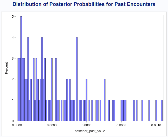
/* Distribution histograms for the posterior probabilities */ proc sgplot data=bayesian_analysis; histogram posterior_past_value / transparency=0.5 fillattrs=(color=blue) binwidth=0.00001; title "Distribution of Posterior Probabilities for Past Encounters"; run;
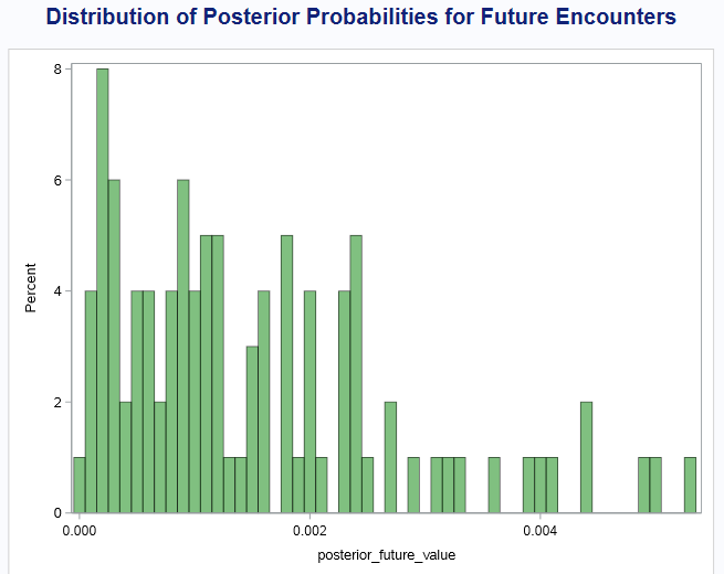
proc sgplot data=bayesian_analysis; histogram posterior_future_value / transparency=0.5 fillattrs=(color=green) binwidth=0.0001; title "Distribution of Posterior Probabilities for Future Encounters"; run;
With this code, we simulate both past and future alien encounters under a range of assumptions, enabling us to estimate the likelihood of each scenario using Bayesian reasoning. By the end of the process, we have distributions of probabilities for both past and future alien contact, which we’ll now analyze to gain further insights.
Analyzing the Table and Graphical Output
Table Output
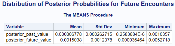
The table presents the summary statistics for the posterior probabilities, which represent the likelihood of both past and future alien encounters:
posterior_past_value:
Mean: 0.000306778
Std Dev: 0.000262715
Minimum: 8.258388E-6
Maximum: 0.0010357
posterior_future_value:
Mean: 0.0015038
Std Dev: 0.0012378
Minimum: 0.000036464
Maximum: 0.0052718
Interpretation:
Past Encounters: The mean probability for past encounters is around 0.0003, or approximately 0.03%. In more intuitive terms, this translates to about a 1 in 3,260 chance that we’ve encountered aliens in the past.
Future Encounters: The mean probability for future encounters is higher, at around 0.0015, or 0.15%. This translates to about a 1 in 667 chance of encountering aliens in the future.
The range of these values indicates that there is quite a bit of uncertainty, which makes sense given the limitations of the data and assumptions. The minimum value for past encounters is as low as 0.000008 (or 1 in 125,000), while the maximum value is closer to 0.001 (or 1 in 1,000). Future encounters range from 0.000036 (1 in 27,397) to 0.005 (or 1 in 190).
Graphical Output
Distribution of Posterior Probabilities for Past Encounters: The histogram shows a wide distribution, with most probabilities clustering around the lower end, below 0.0005. This suggests that the likelihood of past encounters is generally low across our simulations, but there are still a few instances where the probability was higher, approaching 0.001 (or 1 in 1,000).
2. Distribution of Posterior Probabilities for Future Encounters: The distribution for future encounters is more spread out, with the highest probability occurrences clustered between 0.0005 and 0.002. This indicates that future encounters, while still unlikely, have a higher probability than past encounters. The shape of the distribution suggests that while the odds of contact are low, there is a non-trivial chance that future encounters could happen, depending on how certain assumptions play out.
Key Takeaways and Probability Calculations
Past Encounters:
The mean posterior probability of a past encounter is approximately 0.0003. In terms of simple odds, this translates to a 1 in 3,260 chance that humanity has already encountered extraterrestrial life without realizing it. The wide distribution reflects uncertainty, with probabilities ranging from as low as 1 in 125,000 to as high as 1 in 1,000, depending on the assumptions we use for prior likelihoods and evidence.
Future Encounters:
The mean posterior probability for future encounters is 0.0015, which translates to a 1 in 667 chance that we will encounter alien life at some point in the future. While still unlikely, this higher probability compared to past encounters suggests a better (though still slim) chance of future contact. The distribution ranges from a 1 in 27,397 chance at the low end to a more optimistic 1 in 190 chance, reflecting the wide range of possible outcomes.
Tying It All Together: What Does This Mean?
The journey we’ve taken throughout this series has been a fascinating exploration of probability, uncertainty, and the grandest of questions: Are we alone in the universe? Using the Drake Equation as a framework, we’ve examined every step from the formation of habitable planets to the development of intelligent, communicative civilizations. But what does it all mean, and why did we take this approach?
The Bigger Picture
Why We Did This: Our goal was simple, yet profound: to rationally assess the likelihood of alien civilizations existing and, even more importantly, whether we have — or will ever — encounter them. There is a lot of speculation in popular culture about UFOs, sightings, and mysterious signals, but we wanted to approach this scientifically. By working through the Drake Equation, using Monte Carlo simulations, and applying Bayesian reasoning, we attempted to put some tangible numbers to an otherwise nebulous question.
How We Did It: The methodology we used isn’t about definitive answers but rather about understanding the range of possibilities. Each step of the Drake Equation brings with it huge uncertainties — how many habitable planets exist, how many develop life, and how many civilizations are sending signals into the cosmos. To handle this uncertainty, we turned to Monte Carlo simulations, which allowed us to account for a broad range of outcomes and calculate distributions instead of single estimates. Bayesian analysis then helped us refine these probabilities based on current evidence — or the lack thereof — providing more nuanced predictions about alien contact.
What the Results Mean: The numbers might seem small at first glance, but they are significant in their implications. The odds of past contact (about 1 in 3,260) are low, which isn’t surprising given the lack of definitive evidence. Yet, these odds are not zero, and that in itself is worth noting — there is a chance, however small, that we have already encountered extraterrestrial life without realizing it.
The probability of future contact is a bit more optimistic: around 1 in 667. While still a long shot, this suggests that if we continue searching, there is a small but tangible chance we could detect or communicate with alien civilizations at some point in the future. The future is uncertain, but with advancing technology and an ever-expanding field of study in astrobiology and space exploration, the possibility remains.
The Takeaway:
This analysis leaves us with a sobering but hopeful conclusion. The universe is vast, and the distances between stars — let alone civilizations — are staggering. The very structure of the cosmos, combined with the timescales involved in the rise and fall of civilizations, suggests that encounters are improbable but not impossible.
The true marvel here is not just in the numbers but in what they represent: the intersection of humanity’s curiosity and our capacity for rational, evidence-based exploration. We may be alone, or we may one day share a signal with another intelligent civilization. Either way, the work we’ve done to quantify the probabilities shows that the search itself is worthwhile. It reveals how much we still have to learn about the universe and our place in it.
While the odds may not be in our favor, the possibility of a future encounter — however remote — gives us reason to keep looking to the stars. The universe remains full of mysteries, and our journey to solve them continues. Whether or not we ever make contact, the search itself pushes the boundaries of science, philosophy, and our collective imagination.
This is where the work leaves us — not with concrete answers, but with profound questions that will continue to inspire curiosity, exploration, and wonder for generations to come. The search for extraterrestrial life is a search for understanding, not just of the cosmos, but of ourselves.
Unless otherwise noted, all images are by the author
Are We Alone? was originally published in Towards Data Science on Medium, where people are continuing the conversation by highlighting and responding to this story.
How Far Are We from Alien Civilizations? (Part 4 of the Drake Equation Series)
Recap:
In our journey so far, we’ve walked through the Drake Equation to estimate how many civilizations might be “out there” in our galaxy. We’ve covered the stars, the planets that could support life, and how many might develop intelligent civilizations. In Part 3, we estimated how many of those civilizations are capable of communicating with us right now. Now, in Part 4, we’re facing the big question: How far away are they?
The Milky Way is vast. We know there could be thousands of civilizations out there, but the galaxy is 100,000 light-years across — so even if they exist, could we ever hear from them? This article explores the mind-bending distances between us and these potential civilizations, and what that means for our search for extraterrestrial life.
All images were developed by the author using Midjourney.
How Big is Space? Putting the Vastness of the Milky Way into Perspective
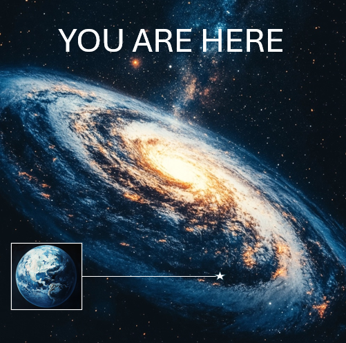
To put the vastness of space into perspective, let’s start by imagining the Milky Way galaxy, which spans about 100,000 light-years in diameter. Now, if we were to shrink the galaxy down to the size of Earth (with a diameter of about 12,742 kilometers), the relative size of Earth itself would become unimaginably small. In fact, Earth would be 742 billion times smaller in comparison — about the size of a single human red blood cell. This comparison illustrates just how immense our galaxy is and emphasizes the monumental challenge of exploring or communicating across such vast distances. Imagine the difficulty of trying to find a single red blood cell in a space the size of the Earth!
Step 8: Estimating the Distance to the Nearest Alien Civilization
The results from Part 3 suggested that there could be up to 2,363 alien civilizations communicating in our galaxy right now. But what does that mean in practical terms? If they’re out there, how close is the nearest one?
Why This Step Matters
Even if we know there are thousands of civilizations, distance is a huge hurdle. The farther away they are, the harder it is to detect their signals — or for them to detect ours. If we want to set realistic expectations for contacting these civilizations, we need to know how far away they are. And if they’re hundreds or even thousands of light-years away, it’s going to be tough to communicate in real time. Imagine sending a text, only to get a reply 2,000 years later!
Our Approach
We’re assuming that alien civilizations are randomly distributed throughout the Milky Way. This gives us a nice, even spread across the galaxy’s disk, which has a diameter of around 100,000 light-years and a thickness of 1,300 light-years.
This approach keeps things simple while acknowledging that we’re making some big assumptions. For example, we’re not considering galactic zones that might be more “life-friendly,” and we’re ignoring the idea that some regions might be barren. But for our purposes, this model gives us a solid foundation for calculating the average distance to the nearest civilization.
Code for Step 8: Calculating the Distance to the Nearest Alien Civilization
*********************************************************************** *Calculate the distance to the closest civilization assuming that they *are randomly distributed across the galaxy ***********************************************************************
data closest_civilization; /* Set seed for reproducibility */ call streaminit(123);
/* Calculate distances */ do i = 1 to &num_iterations; /* Generate random coordinates for civilizations */ do j = 1 to &num_civilizations; x = rand("Uniform", -&galactic_radius, &galactic_radius); y = rand("Uniform", -&galactic_radius, &galactic_radius); z = rand("Uniform", -&galactic_height, &galactic_height);
/* Update closest distance if applicable */ if j = 1 then closest_distance = distance; else if distance < closest_distance then closest_distance = distance; end;
/* Store closest distance */ distances[i] = closest_distance; end;
/* Output distances to dataset */ do iteration = 1 to &num_iterations; distance = distances[iteration]; output; end;
/* Keep only the necessary variables */ keep iteration distance; run;
A Small Confession: I Cheated (and Gave Us Better Odds)
Alright, time for a little confession: the Earth isn’t actually sitting in the middle of the galaxy, despite how I set up the code to calculate the distance to the nearest alien civilization. In reality, we’re about three-quarters of the way toward the edge of the Milky Way. If I had placed the Earth where it truly belongs, the average distance to alien civilizations on the far side of the galaxy would be much greater. But by “cheating” and moving us to the galactic center, I’ve inadvertently decreased the average distance to potential neighbors — and, in turn, increased our odds of contact. So yes, this biased approach works in our favor, but I’m sure you won’t mind if I made the cosmos feel a little cozier!
Breaking Down the Code: Calculating the Distance to the Nearest Civilization
This code is designed to simulate and calculate the distance from Earth to the nearest alien civilization, assuming that civilizations are randomly distributed throughout the Milky Way galaxy. Let’s walk through the key components and logic of the code.
Overview of the Key Variables
num_civilizations: This is set to 2,363, which is the number of civilizations we estimated in Part 3 to be communicating at the same time as us. This parameter is the foundation of our calculation, as we want to figure out how far the closest of these civilizations might be from us.
galactic_radius and galactic_height: These parameters define the size of the Milky Way. The galaxy is modeled as a disk, 100,000 light-years in diameter (which gives us a radius of 50,000 light-years) and 1,300 light-years thick.
num_iterations: The code will run 100 iterations of the simulation, meaning it will randomly distribute the civilizations and recalculate the distance multiple times to get a range of possible distances to the nearest civilization.
Setting Up the Simulation
Random Seeding (call streaminit(123)): This is for reproducibility. By setting a seed value (123), we ensure that every time we run this code, we get the same random values, making the results consistent across multiple runs.
Random Galactic Coordinates: Each alien civilization is randomly placed in the galaxy by generating random (x, y, z) coordinates, with x and y representing the positions within the galaxy’s disk (radius), and z representing the position relative to the height of the galaxy (its thickness). The rand(“Uniform”,…) function generates random values within the specified ranges:
The x and y coordinates are picked from a range of -50,000 to +50,000 light-years to cover the full width of the galaxy.
The z coordinate is picked from a range of -1,300 to +1,300 light-years to represent the galaxy’s thickness.
Calculating Distance from Earth
The next section of the code calculates the distance from Earth (located at the origin, [0, 0, 0]) to each randomly positioned alien civilization using the 3D distance formula:
This formula calculates the straight-line distance from Earth to each civilization based on its random galactic coordinates.
Finding the Closest Civilization
Now that we have the distances, the code checks which one is the closest:
First Civilization: On the first iteration (when j = 1), the first calculated distance is stored as the closest distance, because at this point, there’s nothing to compare it to.
Subsequent Civilizations: For each additional civilization, the code compares its distance to the previously stored closest distance. If the new distance is smaller, it updates the value of closest_distance.
Storing and Outputting the Results
Storing the Closest Distance: The closest distance found in each iteration is stored in the array distances[]. This allows us to keep track of the closest civilization for each simulation run.
Output the Distances: The do loop at the end outputs the distance data for each iteration, so we can analyze the distribution of these results. It’s essentially producing a dataset of distances for all 100 simulation runs.
What This Code Is Doing
This simulation is creating random galactic coordinates for 2,363 civilizations in each iteration, calculating the distance to Earth for each one, and identifying the closest civilization. It repeats this process 100 times, giving us a range of possible distances to the nearest alien civilization based on the assumptions we’ve made.
Why This Matters
This is a crucial step in understanding the practical challenge of contacting extraterrestrial civilizations. Even if there are thousands of civilizations, the closest one could still be far beyond our reach. By simulating random distributions, we get an idea of the minimum distance we’d need to cover to contact another civilization — which sets realistic expectations for the search for extraterrestrial life.
Output and Explanation: Distance to the Nearest Civilization
Now for the results! After running the simulation, we get the following estimates for the distance to the nearest alien civilization, based on our earlier calculations:
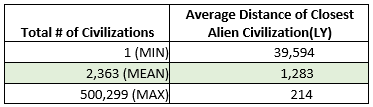
Minimum Number of Civilizations (1): 39,594 light-years away.
Mean Number of Civilizations (2,363): 1,283 light-years away.
Maximum Number of Civilizations (500,299): 214 light-years away.
What Does This Tell Us?
The Closest Possible Civilization: If we take the optimistic scenario where there are half a million alien civilizations, the nearest one would be just over 200 light-years away. This is within a range that we could theoretically detect with current technology, but it’s still a long shot.
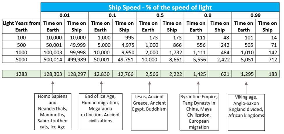
The Most Likely Scenario: With our mean estimate of 2,363 civilizations, the nearest one is likely around 1,283 light-years away. For perspective, that means a signal we send today wouldn’t reach them for over a millennium — and we wouldn’t get a reply until another millennium had passed!
The Worst-Case Scenario: If there’s only one other civilization out there, it could be nearly 40,000 light-years away, making contact almost impossible.
Why This Matters
Even with the exciting possibility of thousands of alien civilizations, the sheer distances between us are daunting. On average, we’re looking at over 1,000 light-years to the nearest civilization, which means that communication is a long shot — at least with our current technology. But that doesn’t mean the search is hopeless. It just means we need to adjust our expectations and think about more indirect ways to detect signs of intelligent life.
Step 9: Traveling the Cosmic Distances — The Role of Relativity
So, let’s say we somehow knew where an alien civilization was located. How long would it take to reach them? This is where things get even more mind-bending — because when you’re talking about interstellar distances, you have to think about Einstein’s theory of special relativity.
Understanding the Lorentz Factor
At the heart of special relativity is the Lorentz Factor. This concept explains how time and space behave as objects approach the speed of light, and it’s key to understanding how interstellar travel might work.
Here’s the formula:
Where:
v is the velocity of the spacecraft (or any object moving through space).
c is the speed of light.
What this equation tells us is that as an object’s velocity v gets closer to the speed of light c, the Lorentz Factor γ grows larger. This leads to two key effects:
Time Dilation: Time slows down for the travelers on the spacecraft. If you’re zooming through space at close to light speed, you experience less time than those on Earth. So, a trip that takes thousands of years from Earth’s perspective might only feel like a few years to the travelers.
Length Contraction: The distance to your destination appears shorter. As you approach the speed of light, distances seem to shrink for the people on the spacecraft.
Now, let’s apply this to our scenario.
Code for Step 9: Calculating Travel Time and the Lorentz Factor
***************************************************************; *How long is the travel time given different distances and ; *different "% of speed of light" ; ***************************************************************;
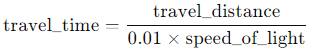
/* Constants */ data _null_; speed_of_light = 299792.458; /* km/s */ distance_ly = 100; /* Light years */ distance_km = distance_ly * 9.461 * 10**12; /* Conversion to kilometers */ travel_distance = distance_km; travel_time = travel_distance / (0.9 * speed_of_light); /* Convert to seconds and reduce top speed of ship to % of the speed of light*/
put "Travel Distance (km): " distance_km; put "Travel Time (seconds): " travel_time;
velocity = travel_distance / travel_time;
lorentz_factor = 1 / sqrt(1 - (velocity**2 / (speed_of_light**2))); proper_time_sp = travel_time / lorentz_factor; /* unit of time experienced on spaceship */ time_dilation_sp = proper_time_sp / (365.25 * 24 * 60 * 60); /* converting to years */ time_earth = travel_time / (365.25 * 24 * 60 * 60); /* converting to years */
put "Velocity: " velocity; put "Lorentz Factor: " lorentz_factor; put "Proper Time (Spaceship): " proper_time_sp " seconds"; put "Time Dilation (Spaceship): " time_dilation_sp " years"; put "Time (Earth): " time_earth " years"; run;
Breaking Down the Code: Calculating Travel Time and Time Dilation
This code is designed to calculate how long it would take a spacecraft to travel between Earth and the nearest alien civilization at a fraction of the speed of light. It also calculates the time dilation experienced by the travelers due to Einstein’s theory of special relativity. Let’s break it down step by step to understand how these calculations work and why they’re important.
Constants and Basic Calculations
Speed of Light:
The speed of light, denoted as speed_of_light, is a well-known constant set at 299,792.458 km/s. This is the maximum speed limit for any object according to the laws of physics, and it forms the basis for our travel calculations.
2. Distance to the Closest Civilization:
We set the distance to the nearest civilization (distance_ly) at 1,283 light years (a placeholder value). This number represents the distance we estimated in earlier steps, based on the distribution of civilizations.
3. Convert Distance to Kilometers:
Since the speed of light is in km/s, we need to convert the distance from light years to kilometers:
A light year is approximately 9.461 trillion kilometers, so this conversion gives us the total distance in kilometers, which is crucial for the travel time calculation.
Calculating Travel Time
Fraction of the Speed of Light:
The example below calculates the travel time based on a ship traveling at 1% of the speed of light. The formula used for travel time is:
This formula converts the total distance to the time it would take the spacecraft to cover that distance at 1% of the speed of light. The output is in seconds, which gives us the most precise calculation.
2. Print Travel Distance and Time:
The program outputs the total distance (in kilometers) and travel time (in seconds) to give us a sense of the scale we’re dealing with.
Special Relativity and Time Dilation
In this part of the code, we’re revisiting Einstein’s theory of special relativity, focusing on time dilation as it relates to interstellar travel. We previously discussed the Lorentz Factor, which plays a crucial role in determining how time slows down for objects moving at speeds close to the speed of light.
But why are we using the Lorentz Factor here?
Why the Lorentz Factor Matters
In the context of interstellar travel, as a spacecraft’s velocity approaches the speed of light, the Lorentz Factor increases dramatically. This has two significant effects:
Time Dilation: The time experienced by the crew aboard the spacecraft would be much shorter than the time experienced by observers on Earth. In essence, while the journey might take centuries or millennia from Earth’s perspective, only a few years could pass for the crew.
Perception of Distance: The faster the spacecraft travels, the shorter the distance appears to those on board. This contraction of space, caused by the Lorentz Factor, means that the crew would perceive the journey as much shorter than the actual distance across space.
Impact on Travel Time
By incorporating the Lorentz Factor, the code allows us to calculate two important results:
Proper Time on the Spaceship: The amount of time the crew would experience while traveling across vast distances. Thanks to time dilation, this will be significantly shorter than the time that passes on Earth.
Time on Earth: The total time it would take from an Earth-bound perspective to reach a distant alien civilization. Even at high speeds, the journey could span centuries or longer.
This is why the Lorentz Factor is critical: it lets us understand how time and space behave at relativistic speeds, giving us a glimpse into the effects that would make long-distance space travel more manageable for the travelers, though still incredibly challenging from an Earth-bound perspective.
Final Output
The code outputs several key insights:
Velocity: The spacecraft’s speed as it approaches a percentage of the speed of light.
Lorentz Factor: How much time dilation is occurring due to the spacecraft’s speed.
Proper Time: The journey’s duration as experienced by the crew.
Time on Earth: How much time would pass for those remaining on Earth while the journey is undertaken.
Why This Matters
This section highlights the staggering complexity of interstellar travel. Even though the crew would experience a much shorter journey thanks to time dilation, the distance between Earth and potential alien civilizations remains immense. The Lorentz Factor illustrates how the laws of physics influence not only the speed of travel but also the perception of time and distance. While time dilation offers a potential advantage for long-distance voyages, the journey to a distant civilization remains a monumental task, requiring technology far beyond what we currently possess.
Output and Explanation: Traveling the Cosmic Distances
Now, we’ve come to the moment of truth — understanding just how long it would take to reach the nearest alien civilization given the vast distances of space and different travel speeds.
Travel Time to the Nearest Civilization
We’ve assumed that the nearest alien civilization is 1,283 light-years away, based on our earlier estimates. Here’s where things get fascinating. The travel time varies dramatically depending on how fast the spacecraft is traveling relative to the speed of light. Let’s explore these numbers:
At 1% the Speed of Light: The journey would take a staggering 128,303 years from Earth’s perspective. To put that into context, Homo sapiens would have been living alongside Neanderthals and saber-toothed cats during the Ice Age if this trip had started that long ago!
At 10% the Speed of Light: The trip would still take 12,830 years from Earth’s point of view — that’s around the time of the end of the Ice Age, when humans began migrating and megafauna like mammoths were going extinct.
At 50% the Speed of Light: We start seeing more manageable numbers. The journey would take 2,566 years from Earth’s perspective, which means that when the spacecraft left, humanity would have been in the time of Jesus, ancient Greece, Egypt, and the rise of Buddhism.
At 90% the Speed of Light: Now we’re getting somewhere! The trip would take 1,425 years from Earth’s perspective. Think about that: when the travelers set off, the Byzantine Empire was at its height, the Tang Dynasty ruled China, and the Maya civilization was flourishing.
At 99% the Speed of Light: The journey now takes just 1,295 years from Earth’s perspective. To put that in context, Vikings were sailing the seas, and Anglo-Saxon kingdoms were being established in what is now England.
But there’s more. These figures show time from Earth’s point of view, but for the astronauts on the spacecraft, time dilation caused by traveling at near-light speeds means they’ll experience much less time passing.
Why Time Dilation is Crucial
As the spacecraft approaches the speed of light, time dilation becomes an extraordinary advantage for the travelers:
At 50% the Speed of Light, while 2,566 years would pass on Earth, the crew would only experience 2,222 years.
At 90% the Speed of Light, while 1,425 years would pass on Earth, the crew would only feel 621 years passing. That’s enough for the journey to span multiple human generations, but it makes the idea of interstellar travel more feasible — at least for those aboard the spacecraft.
At 99% the Speed of Light, this becomes even more dramatic. While the journey would take 1,295 years from Earth’s perspective, the crew would only experience 183 years.
The effect of time dilation means that, for the crew, the journey might feel much shorter, even though centuries or millennia would pass back home on Earth. This is why special relativity is so important in understanding the feasibility of interstellar travel. It’s not just about how long the trip takes — it’s about how time itself is experienced differently depending on the speed you’re traveling at.
Why This Matters
This simulation demonstrates that interstellar travel may be possible, but it’s not without enormous challenges. Time dilation offers an advantage to the crew on the spacecraft, but the vast distances mean that even at near-light speeds, the journey could take centuries or more from Earth’s perspective.
The interplay of distance, speed, and time reveals just how difficult — but also fascinating — it would be to travel across the cosmos. While the travelers may experience only a few hundred years, their destination could still be over a millennium away from Earth’s perspective. This provides a striking reminder of the immense scales involved when contemplating the possibility of contacting alien civilizations.
Transition to Part 5: The Final Challenge — Have We Ever Encountered Alien Life?
Now that we’ve tackled the vast distances between civilizations, we face our final challenge: Could we have already encountered alien life and not known it? Or more excitingly, what are the odds we will encounter alien life in the future? In Part 5, we’ll dive into these probabilities, exploring past and future encounters, and what they mean for the future of humanity and the search for extraterrestrial intelligence.
Stay tuned for the grand finale of the Drake Equation series!
Unless otherwise noted, all images are by the author
Galactic Distances was originally published in Towards Data Science on Medium, where people are continuing the conversation by highlighting and responding to this story.
We use cookies on our website to give you the most relevant experience by remembering your preferences and repeat visits. By clicking “Accept”, you consent to the use of ALL the cookies.
This website uses cookies to improve your experience while you navigate through the website. Out of these, the cookies that are categorized as necessary are stored on your browser as they are essential for the working of basic functionalities of the website. We also use third-party cookies that help us analyze and understand how you use this website. These cookies will be stored in your browser only with your consent. You also have the option to opt-out of these cookies. But opting out of some of these cookies may affect your browsing experience.
Necessary cookies are absolutely essential for the website to function properly. These cookies ensure basic functionalities and security features of the website, anonymously.
Cookie
Duration
Description
cookielawinfo-checkbox-analytics
11 months
This cookie is set by GDPR Cookie Consent plugin. The cookie is used to store the user consent for the cookies in the category "Analytics".
cookielawinfo-checkbox-functional
11 months
The cookie is set by GDPR cookie consent to record the user consent for the cookies in the category "Functional".
cookielawinfo-checkbox-necessary
11 months
This cookie is set by GDPR Cookie Consent plugin. The cookies is used to store the user consent for the cookies in the category "Necessary".
cookielawinfo-checkbox-others
11 months
This cookie is set by GDPR Cookie Consent plugin. The cookie is used to store the user consent for the cookies in the category "Other.
cookielawinfo-checkbox-performance
11 months
This cookie is set by GDPR Cookie Consent plugin. The cookie is used to store the user consent for the cookies in the category "Performance".
viewed_cookie_policy
11 months
The cookie is set by the GDPR Cookie Consent plugin and is used to store whether or not user has consented to the use of cookies. It does not store any personal data.
Functional cookies help to perform certain functionalities like sharing the content of the website on social media platforms, collect feedbacks, and other third-party features.
Performance cookies are used to understand and analyze the key performance indexes of the website which helps in delivering a better user experience for the visitors.
Analytical cookies are used to understand how visitors interact with the website. These cookies help provide information on metrics the number of visitors, bounce rate, traffic source, etc.
Advertisement cookies are used to provide visitors with relevant ads and marketing campaigns. These cookies track visitors across websites and collect information to provide customized ads.