Using OpenCV to auto-detect puzzle and redraw the final answer
LinkedIn introduced a games feature recently, encouraging busy professionals to take a moment out of their day and do something mentally stimulating yet completely relaxing. These games offer a quick break from work and help you reset your mind and return to tasks with even more focus. With these games, LinkedIn aims to foster creativity, improve problem-solving skills, and reignite relationships at work.
In their own words:
Games? On LinkedIn?
Yep. That’s right.
Every year, we study the world’s best workplaces. Turns out, one of the best ways to deepen and reignite relationships at work is simply by having fun together.
So we’re excited to roll out three thinking-oriented games — Pinpoint, Queens, and Crossclimb — that allow you to do just that.
Compete with your connections, spark conversations, and break the ice. Games forge relationships, and relationships are at the heart of everything we do.
The feature initially has got mixed reactions some saying it is swaying away from its core purpose and overall objective, later parts of the reviews have all been positive. Recent articles from The Verge and TechCrunch highlight that games give an escape from the daily grind for a few moments and games in general help develop new neural pathways. Unlike other game apps or sites that push you to constantly keep engaging, LinkedIn games are much simpler and prompt you for attention just once a day.
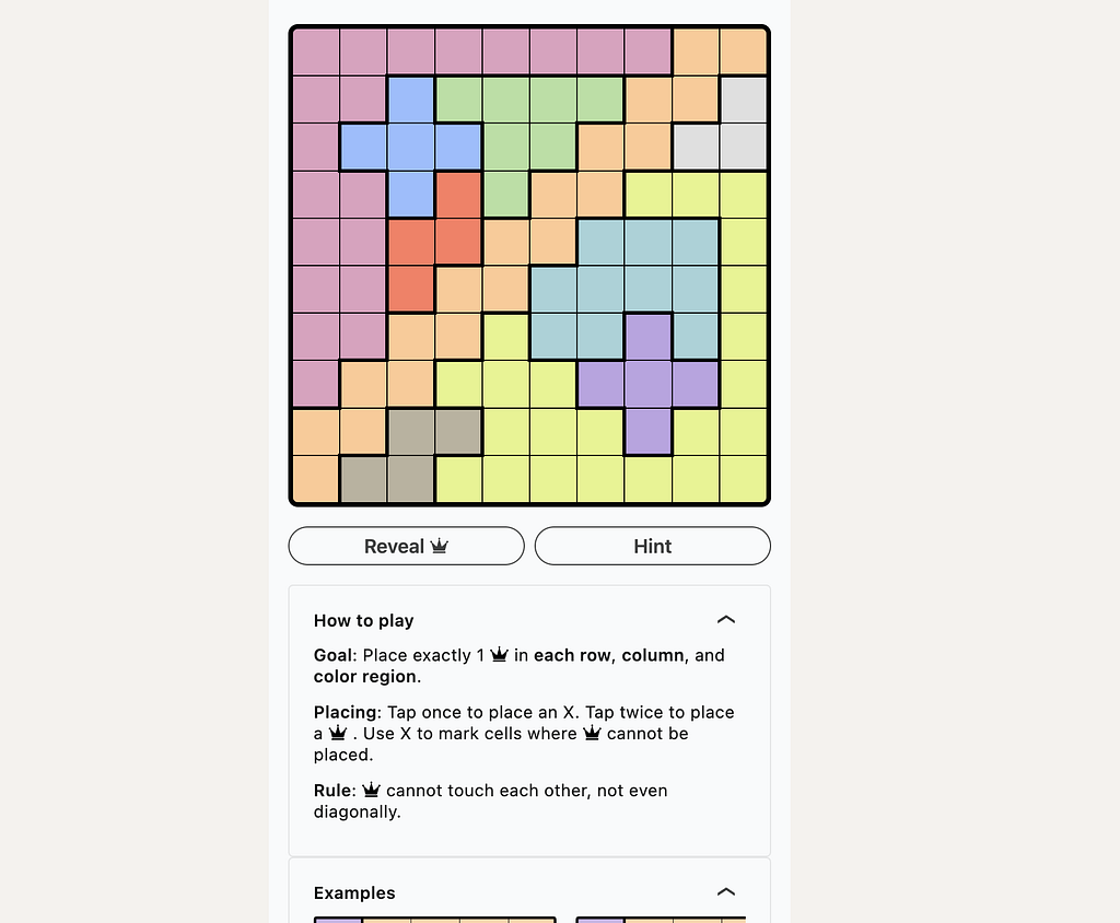
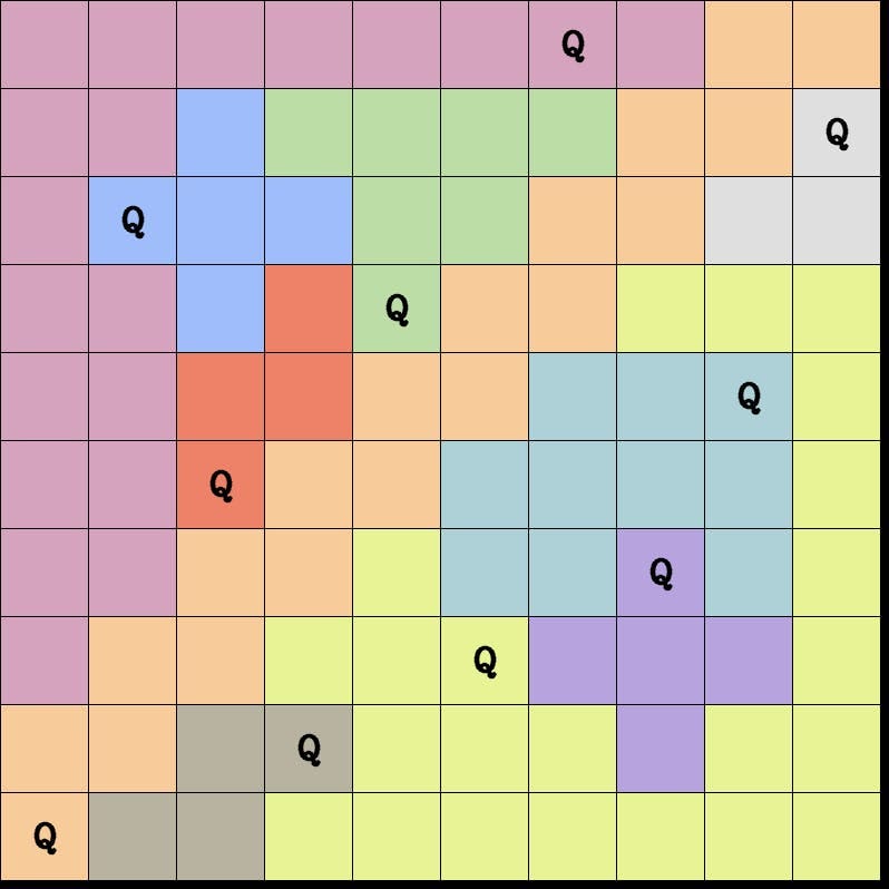
Goal: Place exactly one Q in each row, column, and color region.
Rule: Two Qs cannot touch each other — horizontally, vertically or diagonally
As a weekend project I thought it would be fun to solve Queens game programmatically. The initial idea was to make an LLM solve it, and give us the reasons why it chose a particular cell to place a Q or an X , but thats a topic for another article. In this article, we will explore how to detect a puzzle grid from a screenshot using OpenCV, convert it to a 2D array, and finally solve it using classic, vanilla backtracking, since LinkedIn ensures that there will always be a solution, it means we solve can guarantee that our code will also generate a solution every time.
Final Demo
The idea was:
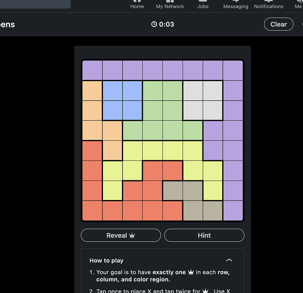
Take a screenshot containing the puzzle
Our code should automatically detect the puzzle grid
Crop or rebuild the puzzle cleanly
Convert the puzzle to a 2D array
Solve the classic n-queens problem using backtracking
Add/Modify the Queens constraints to the N Queens problem
Use the solution to regenerate the image with Queens placed correctly
Enter OpenCV: Detecting and Processing the Puzzle Image
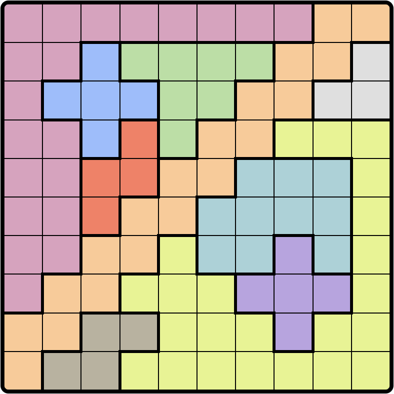
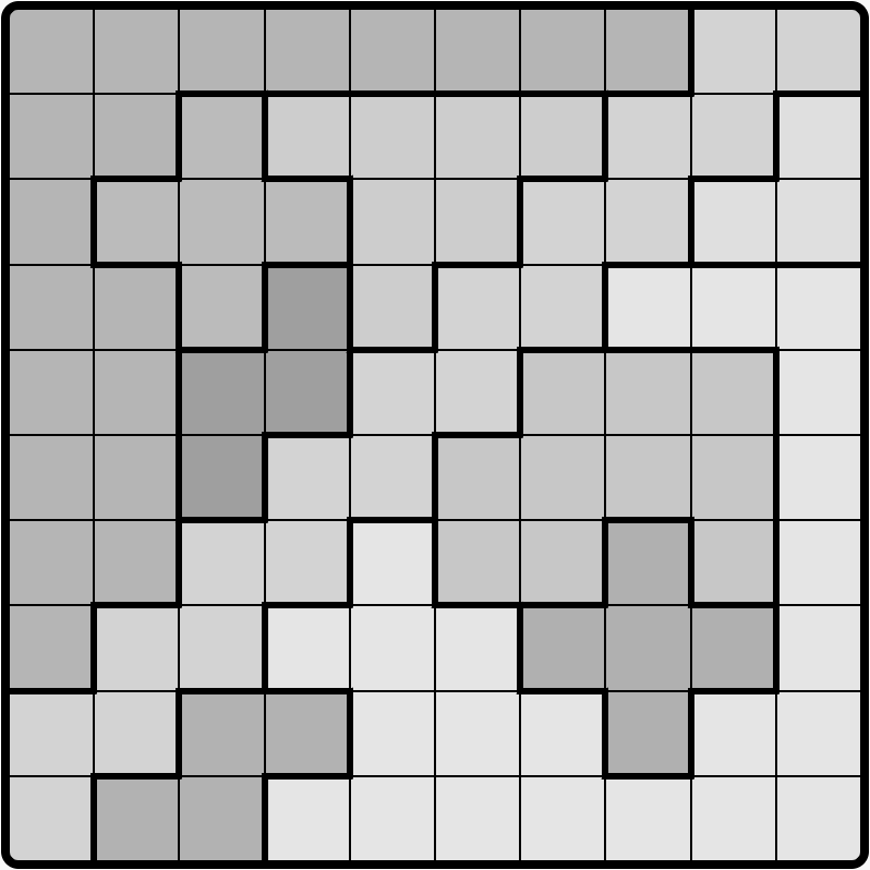
Original screenshot, detected puzzle grid and grayscale of the puzzle
OpenCV (short forOpen Source Computer Vision) is a library for Computer Vision, Machine Learning, and Image Processing. It can be used to identify patterns in an image, extract features, and perform mathematical operations on it. The first step is to process the puzzle screenshot using OpenCV, lets have a quick refresher on basics of OpenCV image processing.
Install the OpenCV python package
pip install opencv-python
How to load an image
cv.imreadreads an image file and converts it to an OpenCV matrix. If the image cannot be read because the file may be missing or in a format that OpenCV can’t understand an empty matrix is returned. The OpenCV matrix can be converted to an image back using cv.imshow function.
import cv2 as cv
import numpy as np

# Reading an image
original = cv.imread("<file_name">)
cv.imshow("original", original)
How to draw a line, circle, rectangle, text on the same image
Once we detect the grid, we need to recreate it using lines and place Qusing text. Let’s look at a short snippet to draw a line, circle, rectangle, and text on the above read matrix.
# Drawing a line
line = cv.line(original, (original.shape[1]//2, original.shape[0]//2), (0,0) , (0,255,0), thickness=2)
cv.imshow("line", line)

# Drawing other shapes
circle = cv.circle(line, (line.shape[1]//2, line.shape[0]//2), 50, (0,0,255), thickness=2)
rect = cv.rectangle(circle, (10,10), (circle.shape[1]//2, circle.shape[0]//2), (255,0,0), thickness=2)
text = cv.putText(rect, "Hi", (rect.shape[1]//2, rect.shape[0]//2), cv.FONT_HERSHEY_SIMPLEX, 1, (255,255,255), thickness=2)

cv.imshow("all shapes", text)
How to detect contours
Contours are simply a shape joining all points of similar color and intensity at a continuous boundary. These are useful when detecting shapes and object outline analysis. We will draw our puzzle grid by detecting the individual cells.
# Its best to convert image to grayscale
# and add a bit of blur for better contour detections
# since our image is mostly a grid we dont need blur

# by default OpenCV reads images as BGR
# as opposed to traditional RGB
gray = cv.cvtConvert(original, cv.COLOR_BGR2GRAY)
contours, _ = cv.findContours(gray, cv.RETR_TREE, cv.CHAIN_APPROX_NONE)
By default, OpenCV reads images as BGR, as opposed to traditional RGB
Cropping an image
For us to eliminate unnecessary areas from screenshots and reduce noise, once we’ve detected our contours
# its essentially selecting the pixels we need from the entire image
cropped = original[0:original.shape[1]//2, 0:original.shape[0]//2]
cv.imshow("cropped", cropped)
Combining the basics
First, we begin by loading the image into memory and converting it into Grayscale. This helps in simplifying contour detection, a general step that is always followed since it reduces the image complexity. Next, we find contours, sort them, and select the largest one. Typically, the first contour is the bound box of the original image, so we use the second largest contour to isolate the puzzle grid. Then, we crop the image just to get the grid and nothing else. We again find contours, since now the noise is reduced, it will detect the grid better. We determine the number of cells within the grid and iterate over each cell, take the average color, and assign a number of each color, which gives us the 2D array of our puzzle
# Read the input image and save the original original = cv.imread(file_name) cv.imwrite("solution/original.png", original)
# Convert the image to grayscale gray = cv.cvtColor(original, cv.COLOR_BGR2GRAY)
# Find contours in the grayscale image and sort them by area contours, _ = cv.findContours(gray, cv.RETR_TREE, cv.CHAIN_APPROX_NONE) contours = sorted(contours, key=cv.contourArea, reverse=True)
# Extract the bounding box of the puzzle grid (using the second largest contour) x, y, w, h = cv.boundingRect(contours[1])
# Crop the grid area from the original image grid = original[y:y+h, x:x+w] cv.imwrite("solution/grid.png", grid)
# Convert the cropped grid to grayscale gray = cv.cvtColor(grid, cv.COLOR_BGR2GRAY) cv.imwrite("solution/gray-grid.png", gray)
# Find contours again in the cropped grayscale grid contours, _ = cv.findContours(gray, cv.RETR_TREE, cv.CHAIN_APPROX_NONE) contours = sorted(contours, key=cv.contourArea)
# Determine the total number of cells in the grid total_cells = len(contours) - 2 grid_size = int(math.sqrt(total_cells))
# Check if the detected cells form a complete square grid if total_cells != grid_size**2: print("Unable to detect full grid! Aborting")
# Calculate individual cell dimensions cell_width = w // grid_size cell_height = h // grid_size
# Iterate through each cell in the grid for i in range(grid_size): row = [] for j in range(grid_size): # Calculate cell coordinates with padding cell_x = j * cell_width cell_y = i * cell_height padding = 15 cell = grid[cell_y+padding:cell_y+cell_height-padding, cell_x+padding:cell_x+cell_width-padding]
# Get the average color of the cell avg_color = cell.mean(axis=0).mean(axis=0) avg_color = avg_color.astype(int) avg_color = tuple(avg_color)
# Map the color to a unique index if not already mapped if avg_color not in color_map: color_map[avg_color] = str(color_index) reverse_color_map[str(color_index)] = avg_color color_index += 1
# Add the color index to the row row.append(color_map[avg_color])
# Add the row to the board board.append(row)
Original screenshot vs detected 2d-array
N-Queen problem
From the Eight Queen wiki
The eight queens puzzle is the problem of placing eight chess queens on an 8×8 chessboard so that no two queens threaten each other; thus, a solution requires that no two queens share the same row, column, or diagonal. There are 92 solutions. The problem was first posed in the mid-19th century. In the modern era, it is often used as an example problem for various computer programming techniques.
This can be solved simply by Backtracking. Here is intuition:
Starting from the leftmost column, we place a Queen on each row, checking for any conflicts with other Queens, if there is a conflict, we move to the previous column, place it in the next row, and continue with the current column. Once we reach the last column and there can be a valid answer, we will find a solution satisfying all conditions. Here is the solution to the classic N Queen (or Eight Queens) problem using backtracking
def is_safe(board, row, col, n):
    # Check this row on the left side for any queens
    for i in range(col):
        if board[row][i] == 'Q':
            return False

    # Check the upper diagonal on the left side for any queens
    for i, j in zip(range(row, -1, -1), range(col, -1, -1)):
        if board[i][j] == 'Q':
            return False

    # Check the lower diagonal on the left side for any queens
    for i, j in zip(range(row, n), range(col, -1, -1)):
        if board[i][j] == 'Q':
            return False

    # If no queens are found in conflict positions, it's safe to place a queen here
    return True

def solve_nqueens_util(board, col, n):
    # If all queens are placed successfully, return True
    if col >= n:
        return True

    # Try placing a queen in each row of the current column
    for i in range(n):
        # Check if placing a queen at (i, col) is safe
        if is_safe(board, i, col, n):
            # Place the queen at (i, col)
            board[i][col] = 'Q'

            # Recur to place queens in the next column
            if solve_nqueens_util(board, col + 1, n):
                return True

            # If placing queen at (i, col) doesn't lead to a solution, remove the queen (backtrack)
            board[i][col] = '.'

    # If no placement is possible in this column, return False
    return False

def solve_nqueens(n):
    # Initialize the board with empty cells represented by '.'
    board = [['.' for _ in range(n)] for _ in range(n)]

    # Start solving from the first column
    if not solve_nqueens_util(board, 0, n):
        return "No solution exists"

    # Return the board with queens placed if a solution is found
    return board

def print_board(board):
    # Print the board in a readable format
    for row in board:
        print(" ".join(row))

# Example usage: Solve the N-Queens problem for an 8x8 board
n = 8
solution = solve_nqueens(n)
if solution != "No solution exists":
    print_board(solution)
else:
    print(solution)
Constraints for LinkedIn Queens
Taking the above code as a starting point, we modify our is_safe method, so there will be at most one Q in a color group. Our new is_safe method becomes:
def is_safe(original_board, board, row, col, queens_in_colors, n):
    # Check the left side of the current row for any queens
    for i in range(col):
        if board[row][i] == 'Q':
            return False

    # Check the upper diagonal on the left side for any queens
    if col - 1 >= 0 and row - 1 >= 0:
        if board[row-1][col-1] == "Q":
            return False

    # Check the lower diagonal on the left side for any queens
    if col - 1 >= 0 and row + 1 < n:
        if board[row+1][col-1] == "Q":
            return False

    # Check the column above the current row for any queens
    for i in range(row):
        if board[i][col] == "Q":
            return False

    # Check if the current color already has a queen
    current_color = original_board[row][col]
    if queens_in_colors[current_color]:
        return False

    # Return True if all checks are passed and it's safe to place a queen
    return True
Re-generating the Image with the Solution
Finally, time to visualize the solution by re-generating the image with Queens correctly placed. This involves drawing rectangles for cells, lines for boundaries, and text for Queens.
# Solve the N-Queens problem on the given board solved_board = solve_n_queens(board)
# Check if the number of detected colors matches the grid size; abort if mismatched if len(color_map) != grid_size: print("Too many colors detected! Aborting")
# Initialize an empty output image to recreate the grid output_image = np.ones((h, w, 3), dtype="uint8")
# Set border and letter sizes for visual elements border_size = 1 letter_height = 10
# Iterate through each cell of the grid for i in range(grid_size): for j in range(grid_size): # Calculate the position of the current cell cell_x = j * cell_width cell_y = i * cell_height
# Retrieve the color for the current cell from the reverse color map color_pick = reverse_color_map.get(board[i][j]) color = (int(color_pick[0]), int(color_pick[1]), int(color_pick[2]))
# Draw the cell with the appropriate color output_image = cv.rectangle( output_image, (cell_x + border_size, cell_y + border_size), (cell_x + cell_width - border_size, cell_y + cell_height - border_size), color, thickness=-1 )
# If a queen is placed in this cell, draw the letter "Q" at the center of the cell if solved_board[i][j] == "Q": output_image = cv.putText( output_image, "Q", (cell_x + cell_width // 2 - letter_height, cell_y + cell_height // 2 + letter_height), cv.FONT_HERSHEY_COMPLEX, 1, (0, 0, 0), lineType=cv.LINE_AA, thickness=2 )
# Save the output image with the solved board displayed cv.imwrite("solution/solve.png", output_image)
final output
Conclusion
We explored programmatically solving LinkedIn’s Queens game using the classic backtracking approach, by first preprocessing the puzzle grid, detecting the gird and converting it to a 2D array using OpenCV and then implementing the solution to classing N-Queen problem and finally modifying the constraints of the N-Queen solution to fit our needs. Finally, we re-generated the puzzle image to visually present the solution using OpenCV.
Practical Lessons from Porting range-set-blaze to this Container-Like Environment
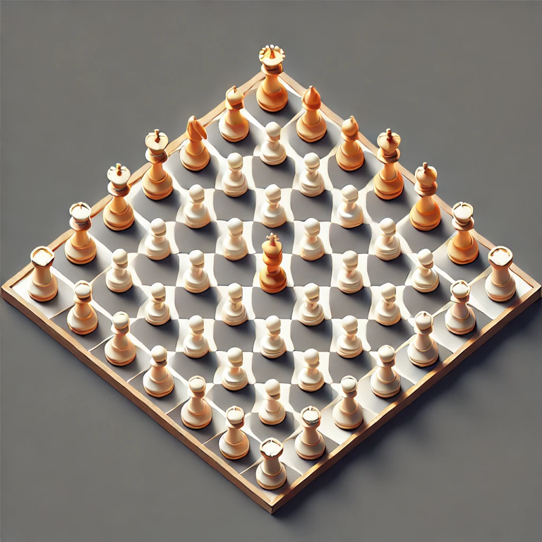
Rust Running on a Container-Like Environment — Source: https://openai.com/dall-e-2/. All other figures from the author.
Do you want your Rust code to run everywhere — from large servers to web pages, robots, and even watches? In this first of three articles, I’ll detail the steps to make that happen.
Running Rust in constrained environments presents challenges. Your code may not have access to a complete operating system such as Linux, Windows, or macOS. You may have limited (or no) access to files, networks, time, random numbers, and even memory. We’ll explore workarounds and solutions.
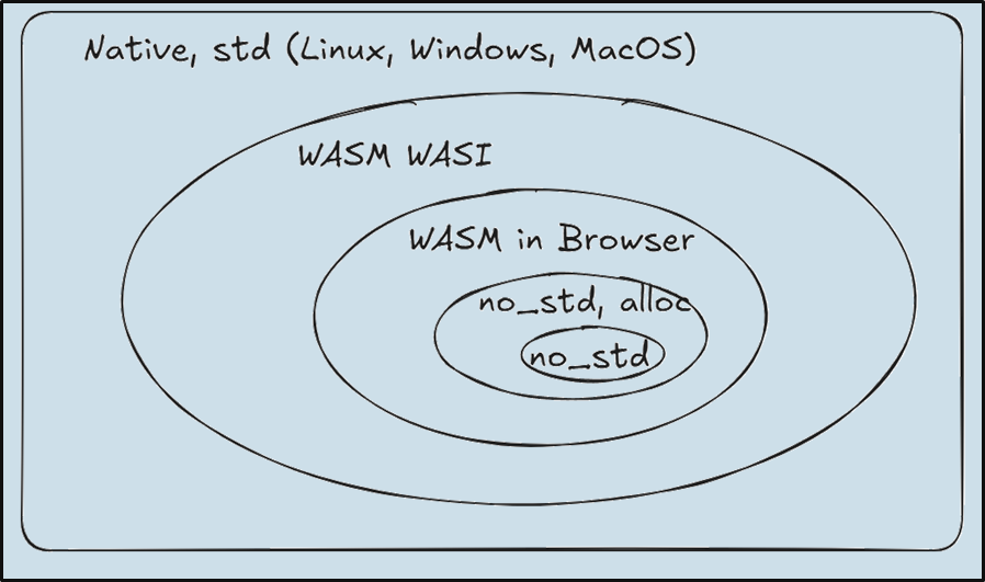
This first article focuses on running code on “WASM WASI”, a container-like environment. We’ll see that WASM WASI may (or may not) be useful in its own right. However, it is valuable as a first step toward running Rust in browsers or embedded systems.
Porting code to run on WASM WASI requires many steps and choices. Navigating these choices can be time consuming. Missing a step can lead to failure. We’ll reduce this complication by offering nine rules, which we’ll explore in detail:
Prepare for disappointment: WASM WASI is easy, but — for now — mostly useless — except as a steppingstone.
Understand Rust targets.
Install the wasm32-wasip1 target and WASMTIME, then create “Hello, WebAssembly!”.
Understand conditional compilation.
Run regular tests but with the WASM WASI target.
Understand Cargo features.
Change the things you can: dependency issues by choosing Cargo features, 64-bit/32-bit issues.
Accept that you cannot change everything: Networking, Tokio, Rayon, etc.
Add WASM WASI to your CI (continuous integration) tests.
Aside: These articles are based on a three-hour workshop that I presented at RustConf24 in Montreal. Thanks to the participants of that workshop. A special thanks, also, to the volunteers from the Seattle Rust Meetup who helped test this material. These articles replace an article I wrote last year with updated information.
Before we look at the rules one by one, let’s define our terms.
WASM: WebAssembly (WASM) is a binary instruction format that runs in most browsers (and beyond).
WASI: WebAssembly System Interface (WASI) allows outside-the-browser WASM to access file I/O, networking (not yet), and time handling.
no_std: Instructs a Rust program not to use the full standard library, making it suitable for small, embedded devices or highly resource-constrained environments.
alloc: Provides heap memory allocation capabilities (Vec, String, etc.) in no_std environments, essential for dynamically managing memory.
With these terms in mind, we can visualize the environments we want our code to run in as a Venn diagram of progressively tighter constraints. This article details how to move from native to WASM WASI. The second article tells how to then move to WASM in the Browser. The final article will cover running Rust in no_std environments, both with and without alloc, ideal for embedded systems.
Based on my experience with range-set-blaze, a data structure project, here are the decisions I recommend, described one at a time. To avoid wishy-washiness, I’ll express them as rules.
Rule 1: Prepare for disappointment: WASM WASI is easy, but — for now — mostly useless — except as a steppingstone.
If WASM+WASI existed in 2008, we wouldn’t have needed to created Docker. That’s how important it is. Webassembly on the server is the future of computing. A standardized system interface was the missing link. Let’s hope WASI is up to the task.
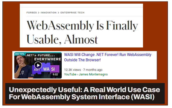
Today, if you follow technology news, you’ll see optimistic headlines like these:
If WASM WASI were truly ready and useful, everyone would already be using it. The fact that we keep seeing these headlines suggests it’s not yet ready. In other words, they wouldn’t need to keep insisting that WASM WASI is ready if it really were.
As of WASI Preview 1, here is how things stand: You can access some file operations, environment variables, and have access to time and random number generation. However, there is no support for networking.
WASM WASI might be useful for certain AWS Lambda-style web services, but even that’s uncertain. Because wouldn’t you prefer to compile your Rust code natively and run twice as fast at half the cost compared to WASM WASI?
Maybe WASM WASI is useful for plug ins and extensions. In genomics, I have a Rust extension for Python, which I compile for 25 different combinations (5 versions of Python across 5 OS targets). Even with that, I don’t cover every possible OS and chip family. Could I replace those OS targets with WASM WASI? No, it would be too slow. Could I add WASM WASI as a sixth “catch-all” target? Maybe, but if I really need portability, I’m already required to support Python and should just use Python.
So, what is WASM WASI good for? Right now, its main value lies in being a step toward running code in the browser or on embedded systems.
Rule 2: Understand Rust targets.
In Rule 1, I mentioned “OS targets” in passing. Let’s look deeper into Rust targets — essential information not just for WASM WASI, but also for general Rust development.
On my Windows machine, I can compile a Rust project to run on Linux or macOS. Similarly, from a Linux machine, I can compile a Rust project to target Windows or macOS. Here are the commands I use to add and check the Linux target to a Windows machine:
Aside: While cargo check verifies that the code compiles, building a fully functional executable requires additional tools. To cross-compile from Windows to Linux (GNU), you’ll also need to install the Linux GNU C/C++ compiler and the corresponding toolchain. That can be tricky. Fortunately, for the WASM targets we care about, the required toolchain is easy to install.
To see all the targets that Rust supports, use the command:
rustc --print target-list
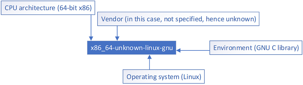
It will list over 200 targets including x86_64-unknown-linux-gnu, wasm32-wasip1, and wasm32-unknown-unknown.
Target names contain up to four parts: CPU family, vendor, OS, and environment (for example, GNU vs LVMM):
Target Name parts — figure from author
Now that we understand something of targets, let’s go ahead and install the one we need for WASM WASI.
Rule 3: Install the wasm32-wasip1 target and WASMTIME, then create “Hello, WebAssembly!”.
To run our Rust code on WASM outside of a browser, we need to target wasm32-wasip1 (32-bit WebAssembly with WASI Preview 1). We’ll also install WASMTIME, a runtime that allows us to run WebAssembly modules outside of the browser, using WASI.
The #[cfg(…)] lines tell the Rust compiler to include or exclude certain code items based on specific conditions. A “code item” refers to a unit of code such as a function, statement, or expression.
With #[cfg(…)] lines, you can conditionally compile your code. In other words, you can create different versions of your code for different situations. For example, when compiling for the wasm32 target, the compiler ignores the #[cfg(not(target_arch = “wasm32”))] block and only includes the following:
fn main() { println!("Hello, WebAssembly!"); }
You specify conditions via expressions, for example, target_arch = “wasm32”. Supported keys include target_os and target_arch. See the Rust Reference for the full list of supported keys. You can also create expressions with Cargo features, which we will learn about in Rule 6.
You may combine expressions with the logical operators not, any, and all. Rust’s conditional compilation doesn’t use traditional if…then…else statements. Instead, you must use #[cfg(…)] and its negation to handle different cases:
To conditionally compile an entire file, place #![cfg(…)] at the top of the file. (Notice the “!”). This is useful when a file is only relevant for a specific target or configuration.
You can also use cfg expressions in Cargo.toml to conditionally include dependencies. This allows you to tailor dependencies to different targets. For example, this says “depend on Criterion with Rayon when not targeting wasm32”.
[target.'cfg(not(target_arch = "wasm32"))'.dev-dependencies] criterion = { version = "0.5.1", features = ["rayon"] }
Aside: For more information on using cfg expressions in Cargo.toml, see my article: Nine Rust Cargo.toml Wats and Wat Nots: Master Cargo.toml formatting rules and avoid frustration | Towards Data Science (medium.com).
Rule 5: Run regular tests but with the WASM WASI target.
It’s time to try to run your project on WASM WASI. As described in Rule 3, create a .cargo/config.toml file for your project. It tells Cargo how to run and test your project on WASM WASI.
[target.wasm32-wasip1]
runner = "wasmtime run --dir ."
Let’s now attempt to run your project’s tests on WASM WASI. Use the following command:
cargo test --target wasm32-wasip1
If this works, you may be done — but it probably won’t work. When I try this on range-set-blaze, I get this error message that complains about using Rayon on WASM.
error: Rayon cannot be used when targeting wasi32. Try disabling default features. --> C:Userscarlk.cargoregistrysrcindex.crates.io-6f17d22bba15001fcriterion-0.5.1srclib.rs:31:1 | 31 | compile_error!("Rayon cannot be used when targeting wasi32. Try disabling default features.");
To fix this error, we must first understand Cargo features.
Rule 6: Understand Cargo features.
To resolve issues like the Rayon error in Rule 5, it’s important to understand how Cargo features work.
In Cargo.toml, an optional [features] section allows you to define different configurations, or versions, of your project depending on which features are enabled or disabled. For example, here is a simplified part of the Cargo.toml file from the Criterion benchmarking project:
[dependencies] #... # Optional dependencies rayon = { version = "1.3", optional = true } plotters = { version = "^0.3.1", optional = true, default-features = false, features = [ "svg_backend", "area_series", "line_series", ] }
This defines four Cargo features: rayon, plotters, html_reports, and cargo_bench_support. Since each feature can be included or excluded, these four features create 16 possible configurations of the project. Note also the special default Cargo feature.
A Cargo feature can include other Cargo features. In the example, the special default Cargo feature includes three other Cargo features — rayon, plotters, and cargo_bench_support.
A Cargo feature can include a dependency. The rayon Cargo feature above includes the rayon crate as a dependent package.
Moreover, dependent packages may have their own Cargo features. For example, the plotters Cargo feature above includes the plotters dependent package with the following Cargo features enabled: svg_backend, area_series, and line_series.
You can specify which Cargo features to enable or disable when running cargo check, cargo build, cargo run, or cargo test. For instance, if you’re working on the Criterion project and want to check only the html_reports feature without any defaults, you can run:
This command tells Cargo not to include any Cargo features by default but to specifically enable the html_reports Cargo feature.
Within your Rust code, you can include/exclude code items based on enabled Cargo features. The syntax uses #cfg(…), as per Rule 4:
#[cfg(feature = "html_reports")] SOME_CODE_ITEM
With this understanding of Cargo features, we can now attempt to fix the Rayon error we encountered when running tests on WASM WASI.
Rule 7: Change the things you can: dependency issues by choosing Cargo features, 64-bit/32-bit issues.
When we tried running cargo test –target wasm32-wasip1, part of the error message stated: Criterion … Rayon cannot be used when targeting wasi32. Try disabling default features. This suggests we should disable Criterion’s rayon Cargo feature when targeting WASM WASI.
To do this, we need to make two changes in our Cargo.toml. First, we need to disable the rayon feature from Criterion in the [dev-dependencies] section. So, this starting configuration:
[dev-dependencies] criterion = { version = "0.5.1", features = ["html_reports"] }
becomes this, where we explicitly turn off the default features for Criterion and then enable all the Cargo features except rayon.
[dev-dependencies] criterion = { version = "0.5.1", features = [ "html_reports", "plotters", "cargo_bench_support"], default-features = false }
Next, to ensure rayon is still used for non-WASM targets, we add it back in with a conditional dependency in Cargo.toml as follows:
[target.'cfg(not(target_arch = "wasm32"))'.dev-dependencies]
criterion = { version = "0.5.1", features = ["rayon"] }
In general, when targeting WASM WASI, you may need to modify your dependencies and their Cargo features to ensure compatibility. Sometimes this process is straightforward, but other times it can be challenging — or even impossible, as we’ll discuss in Rule 8.
Aside: In the next article in this series — about WASM in the Browser — we’ll go deeper into strategies for fixing dependencies.
After running the tests again, we move past the previous error, only to encounter a new one, which is progress!
#[test]
fn test_demo_i32_len() {
    assert_eq!(demo_i32_len(i32::MIN..=i32::MAX), u32::MAX as usize + 1);
                                                  ^^^^^^^^^^^^^^^^^^^^^ attempt to compute
`usize::MAX + 1_usize`, which would overflow
}
The compiler complains that u32::MAX as usize + 1 overflows. On 64-bit Windows the expression doesn’t overflow because usize is the same as u64 and can hold u32::MAX as usize + 1. WASM, however, is a 32-bit environment so usize is the same as u32 and the expression is one too big.
The fix here is to replace usize with u64, ensuring that the expression doesn’t overflow. More generally, the compiler won’t always catch these issues, so it’s important to review your use of usize and isize. If you’re referring to the size or index of a Rust data structure, usize is correct. However, if you’re dealing with values that exceed 32-bit limits, you should use u64 or i64.
Aside: In a 32-bit environment, a Rust array, Vec, BTreeSet, etc., can only hold up to 2³²−1=4,294,967,295 elements.
So, we’ve fixed the dependency issue and addressed a usize overflow. But can we fix everything? Unfortunately, the answer is no.
Rule 8: Accept that you cannot change everything: Networking, Tokio, Rayon, etc.
WASM WASI Preview 1 (the current version) supports file access (within a specified directory), reading environment variables, and working with time and random numbers. However, its capabilities are limited compared to what you might expect from a full operating system.
If your project requires access to networking, asynchronous tasks with Tokio, or multithreading with Rayon, Unfortunately, these features aren’t supported in Preview 1.
Fortunately, WASM WASI Preview 2 is expected to improve upon these limitations, offering more features, including better support for networking and possibly asynchronous tasks.
Rule 9: Add WASM WASI to your CI (continuous integration) tests.
So, your tests pass on WASM WASI, and your project runs successfully. Are you done? Not quite. Because, as I like to say:
If it’s not in CI, it doesn’t exist.
Continuous integration (CI) is a system that can automatically run your tests every time you update your code, ensuring that your code continues to work as expected. By adding WASM WASI to your CI, you can guarantee that future changes won’t break your project’s compatibility with the WASM WASI target.
In my case, my project is hosted on GitHub, and I use GitHub Actions as my CI system. Here’s the configuration I added to .github/workflows/ci.yml to test my project on WASM WASI:
By integrating WASM WASI into CI, I can confidently add new code to my project. CI will automatically test that all my code continues to support WASM WASI in the future.
So, there you have it — nine rules for porting your Rust code to WASM WASI. Here is what surprised me about porting to WASM WASI:
The Bad:
Running on WASM WASI offers little utility today. It, however, holds the potential to be useful tomorrow.
In Rust, there’s a common saying: “If it compiles, it works.” Unfortunately, this doesn’t always hold true for WASM WASI. If you use an unsupported feature, like networking, the compiler won’t catch the error. Instead, it will fail at runtime. For example, this code compiles and runs on WASM WASI but always returns an error because networking isn’t supported.
use std::net::TcpStream;

fn main() {
    match TcpStream::connect("crates.io:80") {
        Ok(_) => println!("Successfully connected."),
        Err(e) => println!("Failed to connect: {e}"),
    }
}
The Good:
Running on WASM WASI is a good first step toward running your code in the browser and on embedded systems.
You can run Rust code on WASM WASI without needing to port to no_std. (Porting to no_std is the topic of the third article of this series.)
You can run standard Rust tests on WASM WASI, making it easy to verify your code.
The .cargo/config.toml file and Rust’s –target option make it incredibly straightforward to configure and run your code on different targets—including WASM WASI.
Stay tuned! In the next article, I’ll show you how to port your Rust code to run on WASM in the browser — an ability I find super useful. After that, the final article will explain porting code to embedded systems, which I find incredibly cool.
Aside: Interested in future articles? Please follow me on Medium. I write about Rust and Python, scientific programming, machine learning, and statistics. I tend to write about one article per month.
Few groups of people can be as challenging to understand as members of a National Congress. In almost any country in the world, the figure of the hypocritical politician is infamous among the population. Backroom dealings and beige envelopes are ever-present in political drama series. At the same time, they are one of the most crucial groups to comprehend, as their actions directly impact the country’s future.
To understand Congress, I will base myself on the popular saying — judge people by their actions, not words. Therefore, I will compare and group members of Congress based on their voting history. In this way, we can uncover obscure patterns and understand the true dynamic of a National Congress.
For this project, I will focus on my home country’s National Congress — Brazil’s Camara dos Deputados — but the method can be applied to any country.
Gathering Data
First of all, we need data.
I downloaded data on all the laws voted on and how each member of Congress voted from 2023 to 2024 up to May 18th. All the data is available at the Brazilian Congress’s open data portal. I then created two different pandas dataframes, one with all the laws voted on and another with how each congress member voted in each vote.
To the votacoes dataframe, I selected only the entries with idOrgao of 180, which means they were voted in the main chamber of Congress. So, we have the data for the votes of most congress members. Then I used this the list of the votacoes_Ids to filter the votacoes_votos_dep dataframe.
Now, in the votacoes_votos_dep, each vote is a row with the congress member’s name and the voting session ID to identify who and what the vote refers to. Therefore, I created a pivot table so that each row represents a congress member and each column refers to a vote, encoding Yes as 1 and No as 0 and dropping any vote where more than 280 deputies didn’t vote.
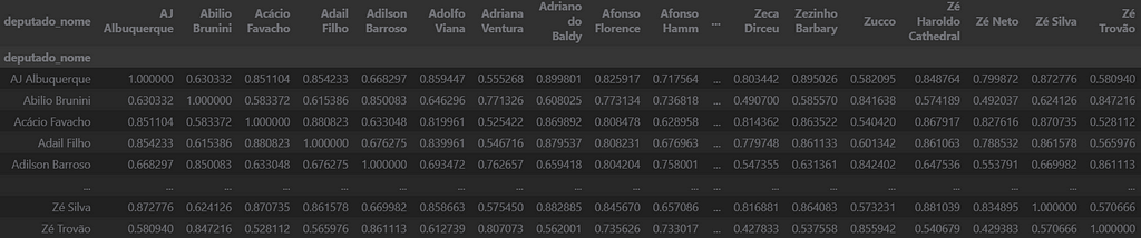
Before computing the similarity matrix, I filled all remaining NAs with 0.5 so as not to interfere with the positioning of the congress member. Finally, we compute the similarity between the vectors of each deputy using cosine similarity and store it in a dataframe.
Now, use the information about the voting similarities between congressmen to build a network using Networkx. A node will represent each member.
import networkx as nx

names = similarity_df.columns
# Create the graph as before
G = nx.Graph()
for i, name in enumerate(names):
    G.add_node(name)
Then, the edges connecting two nodes represent a similarity of at least 75% of the two congressmen’s voting behavior. Also, to address the fact that some congress members have dozens of peers with high degrees of similarity, I only selected the first 25 congressmen with the highest similarity to be given an edge.
threshold = 0.75
for i in range(len(similarity_matrix)):
    for j in range(i + 1, len(similarity_matrix)):
        if similarity_matrix[i][j] > threshold:
            # G.add_edge(names[i], names[j], weight=similarity_matrix[i][j])
            counter[names[i]].append((names[j], similarity_matrix[i][j]))
for source, target in counter.items():
    selected_targets = sorted(target, key=lambda x: x[1], reverse=True)[:26]
    for target, weight in selected_targets:
        G.add_edge(source, target, weight=weight)
To visualize the network, you need to decide the position of each node in the plane. I decided to use the spring layout, which uses the edges as springs holding nodes close while trying to separate. Adding a seed allows for reproducibility since it is a random process.
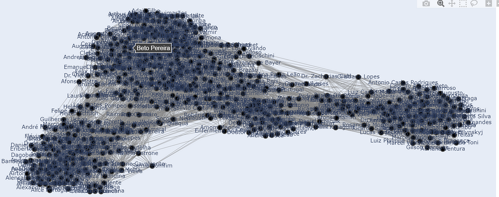
Well, it’s a good start. Different clusters of congressmen can be seen, which suggests that it accurately captures the political alignment and alliances in Congress. But it is a mess, and it is impossible to really discern what’s going on.
To improve the visualization, I made the name appear only when you hover over the node. Also, I colored the nodes according to the political parties and coalitions available on Congress’s site and sized them based on how many edges they are connected to.
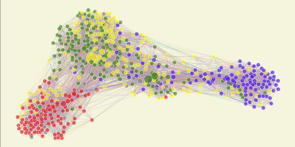
Image by the Author
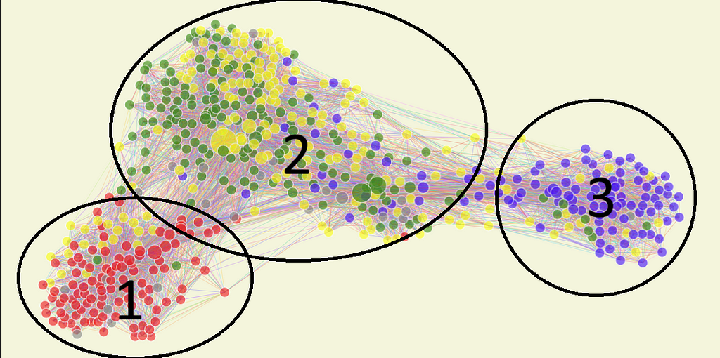
It’s a lot better. We have three clusters, with some nodes between them and a few bigger ones in each. Also, in each cluster, there is a majority of a particular color. Well, let’s dissect it.
Interpreting the Results
First of all, let me explain the colors. Red represents the base of the current left-wing government, so the congressmen of the party of the president or public allies, PT, PSOL, PCdoB, and others. Blue is the opposition led by PL, the party of the ex-president, and another right-wing party, NOVO.
Green and Yellow represent a phenomenon in Brazil’s politics called “Centrao” or “big center.” Centrao is compromised by non-aligned political parties that are always allied with the current government and trade their support for appointments to positions in government or public companies. The Yellow represents the group centered around UNIAO, Brazil’s biggest political party. Green is centered around MDB, a historical party that used to be in charge of most of the “Centrao.”
So, back to the graph:
Image by the Author
Group 1 seems to be mostly composed of red, the current government, and its closest allies. The yellow dots inside are mostly from AVNATE, which, despite publicly being in the same alliance as UNIAO, seems to be more politically aligned with the left.
Another interesting dynamic the network model captures is the grouping of specific parties and ideologies inside each more extensive community. In group 1, right below the base of the number 1, seven nodes are very close to each other. They represent the congress members from PSOL, a radical left party. It’s interesting to see that even inside the left-wing block, they are represented in a sort of sub-group in the network.
Group 2 seems to be mostly compromised from what we can call “Centrao,” as explained before. As always, they are part of the government’s base; they are closer to group 1 than 3, and we can see a mix of Green and yellow, as expected, and some Blue dots. That means many members of Congress who should be in the opposition vote similarly to the government. Why? Well, PL, the current “opposition” party, used to be an average “Centrao” party. Hence, historical members still behave like the average “Centrao”.
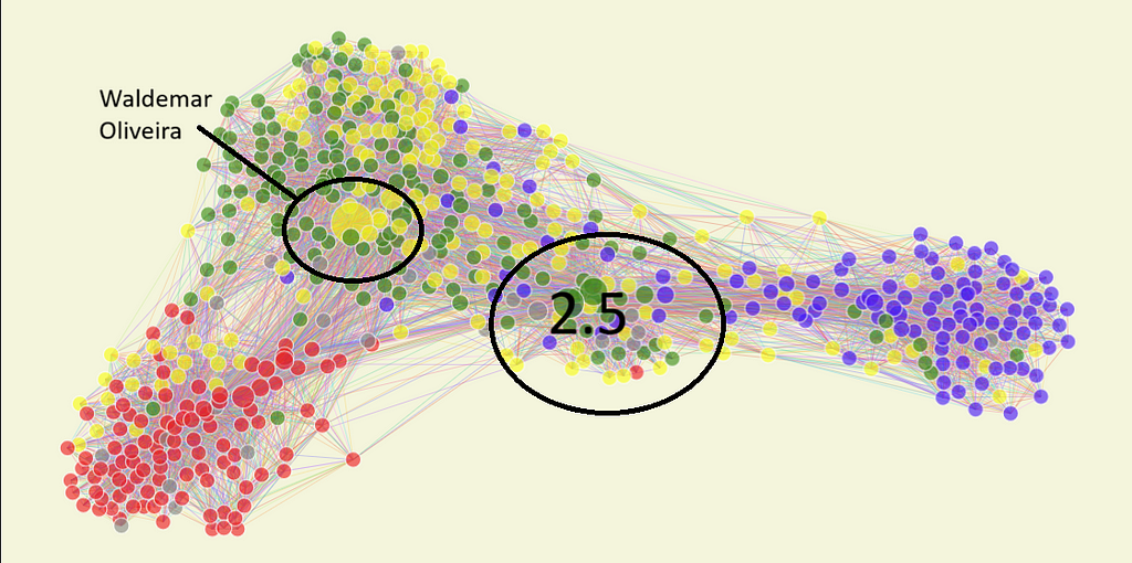
Notably, we have the biggest nodes in group 2. One is yellow and represents Waldemar Oliveira, the leader of the government in the house. He is relevant in Congress, as a big part of it votes according to his directives. The other two biggest nodes are also in group 2, but in what I call group 2.5.
Image by the Author
The reason behind Group 2.5’s behavior is beyond the article; to summarize, it is a group of congressmen who were elected identifying as “right-wing” but still behave more like “Centrao.” Only occasionally do they vote with the right, hence their proximity to Group 3, but whenever votes that interest Group 2 come up, they break away to vote with Group 2.
Finally, group 3 has a different distribution than the other two. It is the smallest one in Congress and is compromised overwhelmingly by PL deputies. It is more “spread out” as there are a lot of members between them and group 2, showing that they do not always vote together. At the same time, there are no oversized nodes, so no clear leader exerts influence on the whole block. This pattern makes sense and aligns with reality since the opposition hasn’t been able to achieve much success in the current Congress.
Conclusion
In conclusion, using networks to analyze the Brazilian Congress yielded valuable insights into political alignments and voting behaviors. Our visualization of voting patterns has revealed three distinct groups: the government’s base, the “Centrao,” and the opposition. The graph effectively illustrates the nuanced relationships between parties, exposing deviations from public stances and highlighting influential figures.
This data-driven approach enhances our understanding of political dynamics, providing a clear visual representation of the complex interplay within the legislative body. By utilizing such analytical tools, we can promote greater transparency in the political process and facilitate more informed discussions about a country’s political situation.
Now that the graph is ready, we can use it to answer questions like:
When does the Centrao vote with the government or the opposition?
Is there a connection between the importance of the network and spending on employees?
Is there a correlation between alignment in the network and geographival location?
If you liked the article and want to read other insights about politics analyzed with data science, follow me here, and don’t miss out. Thank you for reading.
Let me know in the comments what you think of this methodology to analyze political dynamics and if I did anything wrong.
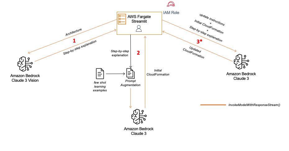
In this post, we explore some ways you can use Anthropic’s Claude 3 Sonnet’s vision capabilities to accelerate the process of moving from architecture to the prototype stage of a solution.
We use cookies on our website to give you the most relevant experience by remembering your preferences and repeat visits. By clicking “Accept”, you consent to the use of ALL the cookies.
This website uses cookies to improve your experience while you navigate through the website. Out of these, the cookies that are categorized as necessary are stored on your browser as they are essential for the working of basic functionalities of the website. We also use third-party cookies that help us analyze and understand how you use this website. These cookies will be stored in your browser only with your consent. You also have the option to opt-out of these cookies. But opting out of some of these cookies may affect your browsing experience.
Necessary cookies are absolutely essential for the website to function properly. These cookies ensure basic functionalities and security features of the website, anonymously.
Cookie
Duration
Description
cookielawinfo-checkbox-analytics
11 months
This cookie is set by GDPR Cookie Consent plugin. The cookie is used to store the user consent for the cookies in the category "Analytics".
cookielawinfo-checkbox-functional
11 months
The cookie is set by GDPR cookie consent to record the user consent for the cookies in the category "Functional".
cookielawinfo-checkbox-necessary
11 months
This cookie is set by GDPR Cookie Consent plugin. The cookies is used to store the user consent for the cookies in the category "Necessary".
cookielawinfo-checkbox-others
11 months
This cookie is set by GDPR Cookie Consent plugin. The cookie is used to store the user consent for the cookies in the category "Other.
cookielawinfo-checkbox-performance
11 months
This cookie is set by GDPR Cookie Consent plugin. The cookie is used to store the user consent for the cookies in the category "Performance".
viewed_cookie_policy
11 months
The cookie is set by the GDPR Cookie Consent plugin and is used to store whether or not user has consented to the use of cookies. It does not store any personal data.
Functional cookies help to perform certain functionalities like sharing the content of the website on social media platforms, collect feedbacks, and other third-party features.
Performance cookies are used to understand and analyze the key performance indexes of the website which helps in delivering a better user experience for the visitors.
Analytical cookies are used to understand how visitors interact with the website. These cookies help provide information on metrics the number of visitors, bounce rate, traffic source, etc.
Advertisement cookies are used to provide visitors with relevant ads and marketing campaigns. These cookies track visitors across websites and collect information to provide customized ads.