
An alternative approach to the transformer for text generation
Originally appeared here:
Attention (is not) all you need
An alternative approach to the transformer for text generation
Originally appeared here:
Attention (is not) all you need
This is the first post in a larger series on Multimodal AI. A Multimodal Model (MM) is an AI system capable of processing or generating multiple data modalities (e.g., text, image, audio, video). In this article, I will discuss a particular type of MM that builds on top of a large language model (LLM). I’ll start with a high-level overview of such models and then share example code for using LLaMA 3.2 Vision to perform various image-to-text tasks.

Large language models (LLMs) have marked a fundamental shift in AI research and development. However, despite their broader impacts, they are still fundamentally limited.
Namely, LLMs can only process and generate text, making them blind to other modalities such as images, video, audio, and more. This is a major limitation since some tasks rely on non-text data, e.g., analyzing engineering blueprints, reading body language or speech tonality, and interpreting plots and infographics.
This has sparked efforts toward expanding LLM functionality to include multiple modalities.
A Multimodal Model (MM) is an AI system that can process multiple data modalities as input or output (or both) [1]. Below are a few examples.
While there are several ways to create models that can process multiple data modalities, a recent line of research seeks to use LLMs as the core reasoning engine of a multimodal system [2]. Such models are called multimodal large language models (or large multimodal models) [2][3].
One benefit of using existing LLM as a starting point for MMs is that they’ve demonstrated a strong ability to acquire world knowledge through large-scale pre-training, which can be leveraged to process concepts appearing in non-textual representations.
Here, I will focus on multimodal models developed from an LLM. Three popular approaches are described below.
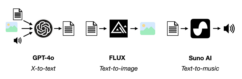
The simplest way to make an LLM multimodal is by adding external modules that can readily translate between text and an arbitrary modality. For example, a transcription model (e.g. Whisper) can be connected to an LLM to translate input speech into text, or a text-to-image model can generate images based on LLM outputs.
The key benefit of such an approach is simplicity. Tools can quickly be assembled without any additional model training.
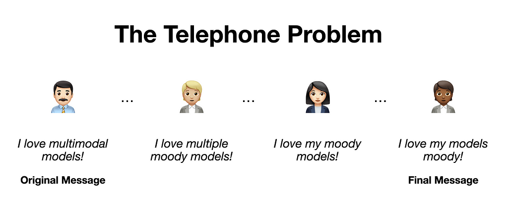
The downside, however, is that the quality of such a system may be limited. Just like when playing a game of telephone, messages mutate when passed from person to person. Information may degrade going from one module to another via text descriptions only.
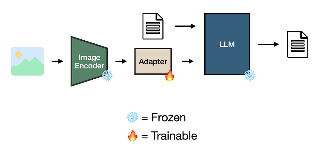
One way to mitigate the “telephone problem” is by optimizing the representations of new modalities to align with the LLM’s internal concept space. For example, ensuring an image of a dog and the description of one look similar to the LLM.
This is possible through the use of adapters, a relatively small set of parameters that appropriately translate a dense vector representation for a downstream model [2][4][5].
Adapters can be trained using, for example, image-caption pairs, where the adapter learns to translate an image encoding into a representation compatible with the LLM [2][4][6]. One way to achieve this is via contrastive learning [2], which I will discuss more in the next article of this series.
The benefits of using adapters to augment LLMs include better alignment between novel modality representations in a data-efficient way. Since many pre-trained embedding, language, and diffusion models are available in today’s AI landscape, one can readily fuse models based on their needs. Notable examples from the open-source community are LLaVA, LLaMA 3.2 Vision, Flamingo, MiniGPT4, Janus, Mini-Omni2, and IDEFICS [3][5][7][8].
However, this data efficiency comes at a price. Just like how adapter-based fine-tuning approaches (e.g. LoRA) can only nudge an LLM so far, the same holds in this context. Additionally, pasting various encoders and decoders to an LLM may result in overly complicated model architectures.
The final way to make an LLM multimodal is by incorporating multiple modalities at the pre-training stage. This works by adding modality-specific tokenizers (rather than pre-trained encoder/decoder models) to the model architecture and expanding the embedding layer to accommodate new modalities [9].
While this approach comes with significantly greater technical challenges and computational requirements, it enables the seamless integration of multiple modalities into a shared concept space, unlocking better reasoning capabilities and efficiencies [10].
The preeminent example of this unified approach is (presumably) GPT-4o, which processes text, image, and audio inputs to enable expanded reasoning capabilities at faster inference times than previous versions of GPT-4. Other models that follow this approach include Gemini, Emu3, BLIP, and Chameleon [9][10].
Training these models typically entails multi-step pre-training on a set of (multimodal) tasks, such as language modeling, text-image contrastive learning, text-to-video generation, and others [7][9][10].
With a basic understanding of how LLM-based multimodal models work under the hood, let’s see what we can do with them. Here, I will use LLaMA 3.2 Vision to perform various image-to-text tasks.
To run this example, download Ollama and its Python library. This enables the model to run locally i.e. no need for external API calls.
The example code is freely available on GitHub.
We start by importing ollama.
import ollama
Next, we’ll download the model locally. Here, we use LLaMA 3.2 Vision 11B.
ollama.pull('llama3.2-vision')
Now, we’re ready to use the model! Here’s how we can do basic visual question answering.
# pass image and question to model
response = ollama.chat(
    model='llama3.2-vision',
    messages=[{
        'role': 'user',
        'content': 'What is in this image?',
        'images': ['images/shaw-sitting.jpeg']
    }]
)

# print response
print(response['message']['content'])
The image is of me from a networking event (as shown below).

The model’s response is shown below. While it has trouble reading what’s on my hat, it does a decent job inferring the context of the photo.
This image shows a man sitting on a yellow ottoman with his hands clasped
together. He is wearing a black polo shirt with a name tag that says "Shaw"
and a black baseball cap with white text that reads, "THE DATA ENREPRENEUR."
The background of the image appears to be an office or lounge area, with a
large screen on the wall behind him displaying a presentation slide. There are
also several chairs and tables in the background, suggesting that this may be
a meeting room or common area for employees to gather and work.
If you run this on your machine, you may run into a long wait time until the model generates a response. One thing we can do to make this less painful is to enable streaming.
# create stream
stream = ollama.chat(
    model='llama3.2-vision',
    messages=[{
        'role': 'user',
        'content': 'Can you write a caption for this image?',
        'images': ['images/shaw-sitting.jpeg']
    }],
    stream=True,
)

# print chunks in stream as they become available
for chunk in stream:
    print(chunk['message']['content'], end='', flush=True)
Interestingly, we get a qualitatively different response when prompting the model in a slightly different way for the same image.
This image features a man sitting on a yellow chair. He is wearing a black
polo shirt with a blue name tag that says "Shaw", khaki pants, and a black
baseball cap with white text that reads "THE DATA ENTHUSIAST". The man has his
hands clasped together in front of him and appears to be smiling.

The background of the image consists of a room with various pieces of
furniture. There is a green ottoman to the left of the yellow chair, and two
blue chairs on the right side of the image. A brown table or desk sits behind
the man, along with a fireplace. The walls are painted teal blue and have a
wooden accent wall featuring holes for hanging items.

The overall atmosphere suggests that this may be a modern office space or
co-working area where people can come to work, relax, or socialize.
Objectively describing a scene is simpler than understanding and explaining humor. Let’s see how the model explains the meme below.

# ask model to explain meme
stream = ollama.chat(
    model='llama3.2-vision',
    messages=[{
        'role': 'user',
        'content': 'Can you explain this meme to me?',
        'images': ['images/ai-meme.jpeg']
    }],
    stream=True,
)

# print stream
for chunk in stream:
    print(chunk['message']['content'], end='', flush=True)
The meme depicts Patrick Star from SpongeBob SquarePants, surrounded by
various AI tools and symbols. The caption reads "Trying to build with AI
today..." The image humorously illustrates the challenges of using AI in
building projects, implying that it can be overwhelming and frustrating.
The model does a good job here. It understands that the image is funny while also conveying the pain that people face.
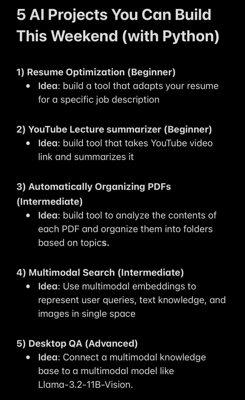
The last use case is optical character recognition (OCR). This involves extracting text from images, which is valuable in a wide range of contexts. Here, I’ll see if the model can translate a screenshot from my notes app to a markdown file.
# ask model to read screenshot and convert to markdown
stream = ollama.chat(
    model='llama3.2-vision',
    messages=[{
        'role': 'user',
        'content': 'Can you transcribe the text from this screenshot in a
                    markdown format?',
        'images': ['images/5-ai-projects.jpeg']
    }],
    stream=True,
)

# read stream
for chunk in stream:
    print(chunk['message']['content'], end='', flush=True)
Here is the transcription of the text in markdown format:

5 AI Projects You Can Build This Weekend (with Python)

1. **Resume Optimization (Beginner)**
 * Idea: build a tool that adapts your resume for a specific job description
2. **YouTube Lecture Summarizer (Beginner)**
 * Idea: build a tool that takes YouTube video links and summarizes them
3. **Automatically Organizing PDFs (Intermediate)**
 * Idea: build a tool to analyze the contents of each PDF and organize them
into folders based on topics
4. **Multimodal Search (Intermediate)**
 * Idea: use multimodal embeddings to represent user queries, text knowledge,
and images in a single space
5. **Desktop QA (Advanced)**
 * Idea: connect a multimodal knowledge base to a multimodal model like
Llama-3.2-11B-Vision

Note that I've added some minor formatting changes to make the text more
readable in markdown format. Let me know if you have any further requests.
Again, the model does a decent job out of the box. While it missed the header, it accurately captured the content and formatting of the project ideas.
YouTube-Blog/multimodal-ai/1-mm-llms at main · ShawhinT/YouTube-Blog
Multimodal models are AI systems that can process multiple data modalities as inputs or outputs (or both). A recent trend for developing these systems consists of adding modalities to large language models (LLMs) in various ways.
However, there are other types of multimodal models. In the next article of this series, I will discuss multimodal embedding models, which encode multiple data modalities (e.g. text and images) into a shared representation space.
My website: https://www.shawhintalebi.com/
Get FREE access to every new story I write
[1] Multimodal Machine Learning: A Survey and Taxonomy
[2] A Survey on Multimodal Large Language Models
[5] Janus: Decoupling Visual Encoding for Unified Multimodal Understanding and Generation
[6] Learning Transferable Visual Models From Natural Language Supervision
[7] Flamingo: a Visual Language Model for Few-Shot Learning
[8] Mini-Omni2: Towards Open-source GPT-4o with Vision, Speech and Duplex Capabilities
[9] Emu3: Next-Token Prediction is All You Need
[10] Chameleon: Mixed-Modal Early-Fusion Foundation Models
Multimodal Models — LLMs that can see and hear was originally published in Towards Data Science on Medium, where people are continuing the conversation by highlighting and responding to this story.
Originally appeared here:
Multimodal Models — LLMs that can see and hear
Go Here to Read this Fast! Multimodal Models — LLMs that can see and hear
Introduced in the landmark 2017 paper “Attention Is All You Need” (Vaswani et al., 2017), the Transformer architecture is widely regarded as one of the most influential scientific breakthroughs of the past decade. At the core of the Transformer is the attention mechanism, a novel approach that enables AI models to comprehend complex structures by focusing on different parts of input sequences based on the task at hand. Originally demonstrated in the world of natural language processing, the success of the Transformers architecture has quickly spread to many other domains, including speech recognition, scene understanding, reinforcement learning, protein structure prediction, and more. However, attention layers are highly resource-intensive, and as these layers become the standard across increasingly large models, the costs associated with their training and deployment have surged. This has created an urgent need for strategies that reduce the computational cost of this core layer so as to increase the efficiency and scalability of Transformer-based AI models.
In this post, we will explore several tools for optimizing attention in PyTorch. Our focus will be on methods that maintain the accuracy of the attention layer. These will include PyTorch SDPA, FlashAttention, TransformerEngine Attention, FlexAttention, and xFormer attention. Other methods that reduce the computational cost via approximation of the attention calculation (e.g., DeepSpeed’s Sparse Attention, Longformer, Linformer, and more) will not be considered. Additionally, we will not discuss general optimization techniques that, while beneficial to attention performance, are not specific to the attention computation itself (e.g., FP8 training, model sharding, and more).
Importantly, attention optimization is an active area of research with new methods coming out on a pretty regular basis. Our goal is to increase your awareness of some of the existing solutions and provide you with a foundation for further exploration and experimentation. The code we will share below is intended for demonstrative purposes only — we make no claims regarding its accuracy, optimality, or robustness. Please do not interpret our mention of any platforms, libraries, or optimization techniques as an endorsement for their use. The best options for you will depend greatly on the specifics of your own use-case.
Many thanks to Yitzhak Levi for his contributions to this post.
To facilitate our discussion, we build a Vision Transformer (ViT)-backed classification model using the popular timm Python package (version 0.9.7). We will use this model to illustrate the performance impact of various attention kernels.
We start by defining a simplified Transformer block that allows for programming the attention function by passing it into its constructor. Since attention implementations assume specific input tensor formats, we also include an option for controlling the format, ensuring compatibility with the attention kernel of our choosing.
# general imports
import os, time, functools

# torch imports
import torch
from torch.utils.data import Dataset, DataLoader
import torch.nn as nn

# timm imports
from timm.models.vision_transformer import VisionTransformer
from timm.layers import Mlp

IMG_SIZE = 224
BATCH_SIZE = 128

# Define ViT settings
NUM_HEADS = 16
HEAD_DIM = 64
DEPTH = 24
PATCH_SIZE = 16
SEQ_LEN = (IMG_SIZE // PATCH_SIZE)**2 # 196

class MyAttentionBlock(nn.Module):
    def __init__(
            self,
            attn_fn,
            format = None,
            dim: int = 768,
            num_heads: int = 12,
            **kwargs
    ) -> None:
        super().__init__()
        self.attn_fn = attn_fn
        self.num_heads = num_heads
        self.head_dim = dim // num_heads
        self.norm1 = nn.LayerNorm(dim)
        self.norm2 = nn.LayerNorm(dim)
        self.qkv = nn.Linear(dim, dim * 3, bias=False)
        self.proj = nn.Linear(dim, dim)
        self.mlp = Mlp(
            in_features=dim,
            hidden_features=dim * 4,
        )
        permute = (2, 0, 3, 1, 4)
        self.permute_attn = functools.partial(torch.transpose,dim0=1,dim1=2)

        if format == 'bshd':
            permute = (2, 0, 1, 3, 4)
            self.permute_attn = nn.Identity()
        self.permute_qkv = functools.partial(torch.permute,dims=permute)

    def forward(self, x_in: torch.Tensor) -> torch.Tensor:
        x = self.norm1(x_in)
        B, N, C = x.shape
        qkv = self.qkv(x).reshape(B, N, 3, self.num_heads, self.head_dim)
        # permute tensor based on the specified format
        qkv = self.permute_qkv(qkv)
        q, k, v = qkv.unbind(0)
        # use the attention function specified by the user
        x = self.attn_fn(q, k, v)
        # permute output according to the specified format
        x = self.permute_attn(x).reshape(B, N, C)
        x = self.proj(x)
        x = x + x_in
        x = x + self.mlp(self.norm2(x))
        return x
We define a randomly generated dataset which we will use to feed to our model during training.
# Use random data
class FakeDataset(Dataset):
    def __len__(self):
        return 1000000

    def __getitem__(self, index):
        rand_image = torch.randn([3, IMG_SIZE, IMG_SIZE],
                                 dtype=torch.float32)
        label = torch.tensor(data=index % 1000, dtype=torch.int64)
        return rand_image, label
Next, we define our ViT training function. While our example focuses on demonstrating a training workload, it is crucial to emphasize that optimizing the attention layer is equally, if not more, important during model inference.
The training function we define accepts the customized Transformer block and a flag that controls the use of torch.compile.
def train_fn(block_fn, compile):
    torch.random.manual_seed(0)
    device = torch.device("cuda:0")
    torch.set_float32_matmul_precision("high")

    # Create dataset and dataloader
    train_set = FakeDataset()
    train_loader = DataLoader(
        train_set, batch_size=BATCH_SIZE,
        num_workers=12, pin_memory=True, drop_last=True)

    model = VisionTransformer(
       img_size=IMG_SIZE,
       patch_size=PATCH_SIZE,
       embed_dim=NUM_HEADS*HEAD_DIM,
       depth=DEPTH,
       num_heads=NUM_HEADS,
       class_token=False,
       global_pool="avg",
       block_fn=block_fn
    ).to(device)

    if compile:
        model = torch.compile(model)

    # Define loss and optimizer
    criterion = torch.nn.CrossEntropyLoss()
    optimizer = torch.optim.SGD(model.parameters())

    model.train()

    t0 = time.perf_counter()
    summ = 0
    count = 0
    for step, data in enumerate(train_loader):
        # Copy data to GPU
        inputs = data[0].to(device=device, non_blocking=True)
        label = data[1].to(device=device, non_blocking=True)
        with torch.amp.autocast('cuda', enabled=True, dtype=torch.bfloat16):
            outputs = model(inputs)
            loss = criterion(outputs, label)
        optimizer.zero_grad(set_to_none=True)
        loss.backward()
        optimizer.step()

        # Capture step time
        batch_time = time.perf_counter() - t0
        if step > 20:  # Skip first steps
            summ += batch_time
            count += 1
        t0 = time.perf_counter()
        if step > 100:
            break
    print(f'average step time: {summ / count}')

# define compiled and uncompiled variants of our train function
train = functools.partial(train_fn, compile=False)
train_compile = functools.partial(train_fn, compile=True)
In the code block below we define a PyTorch-native attention function and use it to train our ViT model:
def attn_fn(q, k, v):
    scale = HEAD_DIM ** -0.5
    q = q * scale
    attn = q @ k.transpose(-2, -1)
    attn = attn.softmax(dim=-1)
    x = attn @ v
    return x

block_fn = functools.partial(MyAttentionBlock, attn_fn=attn_fn)

print('Default Attention')
train(block_fn)
print('Compiled Default Attention')
train_compile(block_fn)
We ran this on an NVIDIA H100 with CUDA 12.4 and PyTorch 2.5.1. The uncompiled variant resulted in an average step time of 370 milliseconds (ms), while the compiled variant improved to 242 ms. We will use these results as a baseline for comparison as we consider alternative solutions for performing the attention computation.
One of the easiest ways to boost the performance of our attention layers in PyTorch is to use the scaled_dot_product_attention (SDPA) function. Currently in beta, PyTorch SDPA consolidates multiple kernel-level optimizations and dynamically selects the most efficient one based on the input’s properties. Supported backends (as of now) include: FlashAttention-2, Memory-Efficient Attention, a C++-based Math Attention, and CuDNN. These backends fuse together high-level operations while employing GPU-level optimizations for increasing compute efficiency and memory utilization.
SDPA is continuously evolving, with new and improved backend implementations being introduced regularly. Staying up to date with the latest PyTorch releases is key to leveraging the most recent performance improvements. For example, PyTorch 2.5 introduced an updated CuDNN backend featuring a specialized SDPA primitive specifically tailored for training on NVIDIA Hopper architecture GPUs.
In the code block below, we iterate through the list of supported backends and assess the runtime performance of training with each one. We use a helper function, set_sdpa_backend, for programming the SDPA backend:
from torch.nn.functional import scaled_dot_product_attention as sdpa

def set_sdpa_backend(backend):
    torch.backends.cuda.enable_flash_sdp(False)
    torch.backends.cuda.enable_mem_efficient_sdp(False)
    torch.backends.cuda.enable_math_sdp(False)
    torch.backends.cuda.enable_cudnn_sdp(False)

    if backend in ['flash_sdp','all']:
        torch.backends.cuda.enable_flash_sdp(True)
    if backend in ['mem_efficient_sdp','all']:
        torch.backends.cuda.enable_mem_efficient_sdp(True)
    if backend in ['math_sdp','all']:
        torch.backends.cuda.enable_math_sdp(True)
    if backend in ['cudnn_sdp','all']:
        torch.backends.cuda.enable_cudnn_sdp(True)

for backend in ['flash_sdp', 'mem_efficient_sdp',
                'math_sdp', 'cudnn_sdp']:
    set_sdpa_backend(backend)
    block_fn = functools.partial(MyAttentionBlock,
                                 attn_fn=sdpa)

    print(f'PyTorch SDPA - {backend}')
    train(block_fn)
    print(f'Compiled PyTorch SDPA - {backend}')
    train_compile(block_fn)
We summarize our interim results in the table below
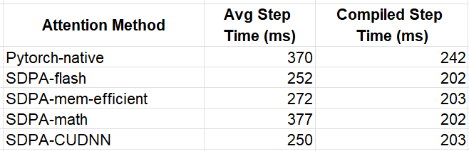
While the choice of SDPA backend has a noticeable impact on performance when running in eager mode, the optimizations performed by model compilation appear to overshadow the differences between the attention kernels. Once again, we caution against deriving any conclusions from these results as the performance impact of different attention functions can vary significantly depending on the specific model and use case.
While PyTorch SDPA is a great place to start, using third-party attention kernels can help accelerate your ML workloads further. These alternatives often come with added flexibility, offering a wider range of configuration options for attention. Some may also include optimizations tailored for specific hardware accelerators or newer GPU architectures.
In this section, we will explore some of the third-party attention kernels available and evaluate their potential impact on runtime performance.
While Pytorch SDPA supports a FlashAttention backend, more advanced FlashAttention implementations can be found in the flash-attn library. Here we will explore the FlashAttention-3 beta release which boasts a speed of up to 2x compared to FlashAttention-2. Given the early stage in its development, FlashAttention-3 can only be installed directly from the GitHub repository and its use is limited to certain head dimensions. Additionally, it does not yet support model compilation. In the following code block, we configure our transformer block to use flash-attn-3 while setting the attention input format to “bshd” (batch, sequence, head, depth) to meet the expectations of the library.
# flash attention 3
from flash_attn_interface import flash_attn_func as fa3
attn_fn = lambda q,k,v: fa3(q,k,v)[0]
block_fn = functools.partial(MyAttentionBlock,
                             attn_fn=attn_fn,
                             format='bshd')

print(f'Flash Attention 3')
train(block_fn)
The resultant step time was 240 ms, making it 5% faster than the SDPA flash-attn.
Transformer Engine (TE) is a specialized library designed to accelerate Transformer models on NVIDIA GPUs. TE is updated regularly with optimizations that leverage the capabilities of the latest NVIDIA hardware and software offerings, giving users access to specialized kernels long before they are integrated into general-purpose frameworks such as PyTorch.
In the code block below we use DotProductAttention from TE version 1.11.0. Similar to PyTorch SDPA, TE supports a number of backends which are controlled via environment variables. Here we demonstrate the use of the NVTE_FUSED_ATTN backend.
def set_te_backend(backend):
    # must be applied before first use of
    # transformer_engine.pytorch.attention
    os.environ["NVTE_FLASH_ATTN"] = '0'
    os.environ["NVTE_FUSED_ATTN"] = '0'
    os.environ["NVTE_UNFUSED_ATTN"] = '0'
    if backend == 'flash':
        os.environ["NVTE_FLASH_ATTN"] = '1'
    if backend == 'fused':
        os.environ["NVTE_FUSED_ATTN"] = '1'
    if backend == 'unfused':
        os.environ["NVTE_UNFUSED_ATTN"] = '1'

from transformer_engine.pytorch.attention import DotProductAttention
set_te_backend('fused')
attn_fn = DotProductAttention(NUM_HEADS, HEAD_DIM, NUM_HEADS,
                              qkv_format='bshd',
                              # disable masking (default is causal mask)
                              attn_mask_type='no_mask')

block_fn = functools.partial(MyAttentionBlock,
                             attn_fn=attn_fn,
                             format='bshd')

print(f'Transformer Engine Attention')
train(block_fn)
print(f'Compiled Transformer Engine Attention')
train_compile(block_fn)
TE attention resulted in average step times of 243 ms and 204 ms for the eager and compiled model variants, correspondingly.
Underlying the memory-efficient backend of PyTorch SDPA is an attention kernel provided by the xFormers library. Once again, we can go to the source to benefit from the latest kernel optimizations and from the full set of API capabilities. In the following code block we use the memory_efficient_attention operator from xFormers version 0.0.28.
# xformer memory efficient attention
from xformers.ops import memory_efficient_attention as mea
block_fn = functools.partial(MyAttentionBlock,
                             attn_fn=mea,
                             format='bshd')

print(f'xFormer Attention ')
train(block_fn)
print(f'Compiled xFormer Attention ')
train_compile(block_fn)
This eager model variant resulted in an average step time of 246 ms, making it 10.5% faster than the SDPA memory efficient kernel. The compiled variant resulted in a step time of 203 ms.
The table below summarizes our experiments:
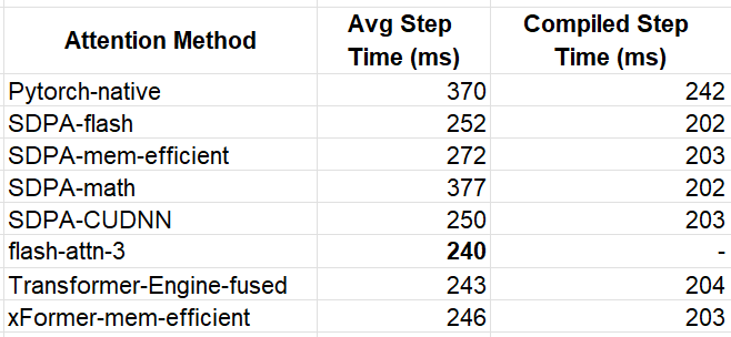
The winner for the eager model was flash-attn-3 with an average step time that is 54% faster than our baseline model. This translates to a similar 54% reduction in training costs. In compiled mode, the performance across the optimized kernels was more or less equal, with the fastest implementations achieving 202 ms, representing a 20% improvement compared to the baseline experiment.
As mentioned above, the precise impact savings is greatly dependent on the model definition. To assess this variability, we reran the experiments using modified settings that increased the attention sequence length to 3136 tokens.
IMG_SIZE = 224
BATCH_SIZE = 8

# Define ViT settings
NUM_HEADS = 12
HEAD_DIM = 64
DEPTH = 6
PATCH_SIZE = 4
SEQ_LEN = (IMG_SIZE // PATCH_SIZE)**2 # 3136
The results are summarized in the table below:
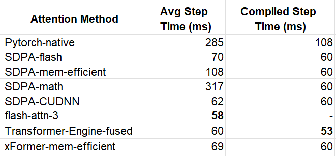
Our immediate observation is that when the sequence length is greater the performance impact of the attention kernels is far more pronounced. Once again, flash-attn-3 came out in front for the eager execution mode — this time with a ~5x increase in performance compared to the PyTorch-native function. For the compiled model we see that the TE kernel broke away from the pack with an overall best step-time of 53 ms.
Thus far, we’ve focused on the standard attention function. However, sometimes we may want to use a variant of the typical attention computation in which we either mask out some of the values of intermediate tensors or apply some operation on them. These types of changes may interfere with our ability to use the optimized attention blocks we covered above. In this section we discuss some of the ways to address this:
Leverage Advanced Kernel APIs
Many optimized attention kernels provide extensive APIs with controls for customizing the attention computation. Before implementing a new solution, explore these APIs to determine if they already support your required functionality.
Implement a custom kernel:
If the existing APIs do not meet your needs, you could consider creating your own custom attention implementation. In previous posts (e.g., here) we discussed some of the pros and cons of custom kernel development. Achieving optimal performance can be extremely difficult. If you do go down this path, one approach might be to start with an existing (optimal) kernel and apply minimal changes to integrate the desired change.
Use FlexAttention:
A recent addition to PyTorch, FlexAttention empowers users to implement a wide variety of attention variants without needing to compromise on performance. Denoting the result of the dot product of the query and key tokens by score, flex_attention allows for programming either a score_mod function or a block_mask mask that is automatically applied to the score tensor. See the documentation as well as the accompanying attention-gym repository for examples of the types of operations that the API enables.
FlexAttention works by compiling the score_mod operator into the attention operator, thereby creating a single fused kernel. It also leverages the sparsity of block_masks to avoid unnecessary computations. The benchmarks reported in the FlexAttention documentation show considerable performance gains for a variety of use cases.
Let’s see both the score_mod and block_mask in action.
Soft-capping is a common technique used to control the logit sizes (e.g., see here). The following code block extends our PyTorch-native attention kernel with soft-capping:
def softcap_attn(q, k, v):
    scale = HEAD_DIM ** -0.5
    q = q * scale
    attn = q @ k.transpose(-2, -1)
    # apply soft-capping
    attn = 30 * torch.tanh(attn/30)
    attn = attn.softmax(dim=-1)
    x = attn @ v
    return x
In the code block below we train our model, first with our PyTorch-native kernel, and then with the optimized Flex Attention API. These experiments were run with the 3136-length sequence settings.
# flex attention imports
from torch.nn.attention.flex_attention import (
    create_block_mask,
    create_mask,
    flex_attention
)
compiled_flex = torch.compile(flex_attention)

# score_mod definition
def tanh_softcap(score, b, h, q_idx, kv_idx):
    return 30 * torch.tanh(score/30)


block_fn = functools.partial(MyAttentionBlock, attn_fn=softcap_attn)

print(f'Attention with Softcap')
train(block_fn)
print(f'Compiled Attention with Softcap')
train_compile(block_fn)

flex_fn = functools.partial(flex_attention, score_mod=tanh_softcap)
compiled_flex_fn = functools.partial(compiled_flex, score_mod=tanh_softcap)

block_fn = functools.partial(MyAttentionBlock,
                             attn_fn=flex_fn)
compiled_block_fn = functools.partial(MyAttentionBlock,
                             attn_fn=compiled_flex_fn)

print(f'Flex Attention with Softcap')
train(compiled_block_fn)
print(f'Compiled Flex Attention with Softcap')
train_compile(block_fn)
The results of the experiments are captured in the table below:
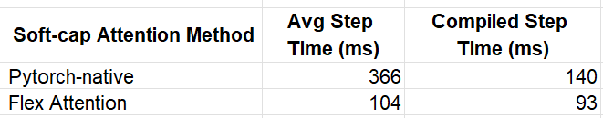
The impact of the Flash Attention kernel is clearly evident, delivering performance boosts of approximately 3.5x in eager mode and 1.5x in compiled mode.
We assess the mask_mod functionality by applying a sparse mask to our attention score. Recall that each token in our sequence represents a patch in our 2D input image. We modify our kernel so that each token only attends to other tokens that our within a 5×5 window in the corresponding 2-D token array.
# convert the token id to a 2d index
def seq_indx_to_2d(idx):
    n_row_patches = IMG_SIZE // PATCH_SIZE
    r_ind = idx // n_row_patches
    c_ind = idx % n_row_patches
    return r_ind, c_ind

# only attend to tokens in a 5x5 surrounding window in our 2D token array
def mask_mod(b, h, q_idx, kv_idx):
    q_r, q_c = seq_indx_to_2d(q_idx)
    kv_r, kv_c = seq_indx_to_2d(kv_idx)
    return torch.logical_and(torch.abs(q_r-kv_r)<5, torch.abs(q_c-kv_c)<5)
As a baseline for our experiment, we use PyTorch SDPA which includes support for passing in an attention mask. The following block includes the masked SDPA experiment followed by the Flex Attention implementation:
# materialize the mask to use in SDPA
mask = create_mask(mask_mod, 1, 1, SEQ_LEN, SEQ_LEN, device='cuda')

set_sdpa_backend('all')
masked_sdpa = functools.partial(sdpa, attn_mask=mask)
block_fn = functools.partial(MyAttentionBlock,
                             attn_fn=masked_sdpa)
print(f'Masked SDPA Attention')
train(block_fn)
print(f'Compiled Masked SDPA Attention')
train_compile(block_fn)

block_mask = create_block_mask(mask_mod, None, None, SEQ_LEN, SEQ_LEN)
flex_fn = functools.partial(flex_attention, block_mask=block_mask)
compiled_flex_fn = functools.partial(compiled_flex, block_mask=block_mask)

block_fn = functools.partial(MyAttentionBlock,
                             attn_fn=flex_fn)
compiled_block_fn = functools.partial(MyAttentionBlock,
                             attn_fn=compiled_flex_fn)

print(f'Masked Flex Attention')
train(compiled_block_fn)
print(f'Compiled Masked Flex Attention')
train_compile(block_fn)
The results of the experiments are captured below:
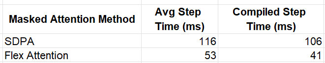
Once again, Flex Attention offers a considerable performance boost, amounting to 2.19x in eager mode and 2.59x in compiled mode.
Although we have succeeded in demonstrating the power and potential of Flex Attention, there are a few limitations that should be noted:
In the face of these limitations, we can return to one of the other optimization opportunities discussed above.
As the reliance on transformer architectures and attention layers in ML models increases, so does the need for tools and techniques for optimizing these components. In this post, we have explored a number of attention kernel variants, each with its own unique properties, capabilities, and limitations. Importantly, one size does not fit all — different models and use cases will warrant the use of different kernels and different optimization strategies. This underscores the importance of having a wide variety tools and techniques for optimizing attention layers.
In a future post, we hope to further explore attention layer optimization by focusing on applying some of the tools we discussed to tackle the challenge of handling variable-sized input sequences. Stay tuned…
Increasing Transformer Model Efficiency Through Attention Layer Optimization was originally published in Towards Data Science on Medium, where people are continuing the conversation by highlighting and responding to this story.
Originally appeared here:
Increasing Transformer Model Efficiency Through Attention Layer Optimization

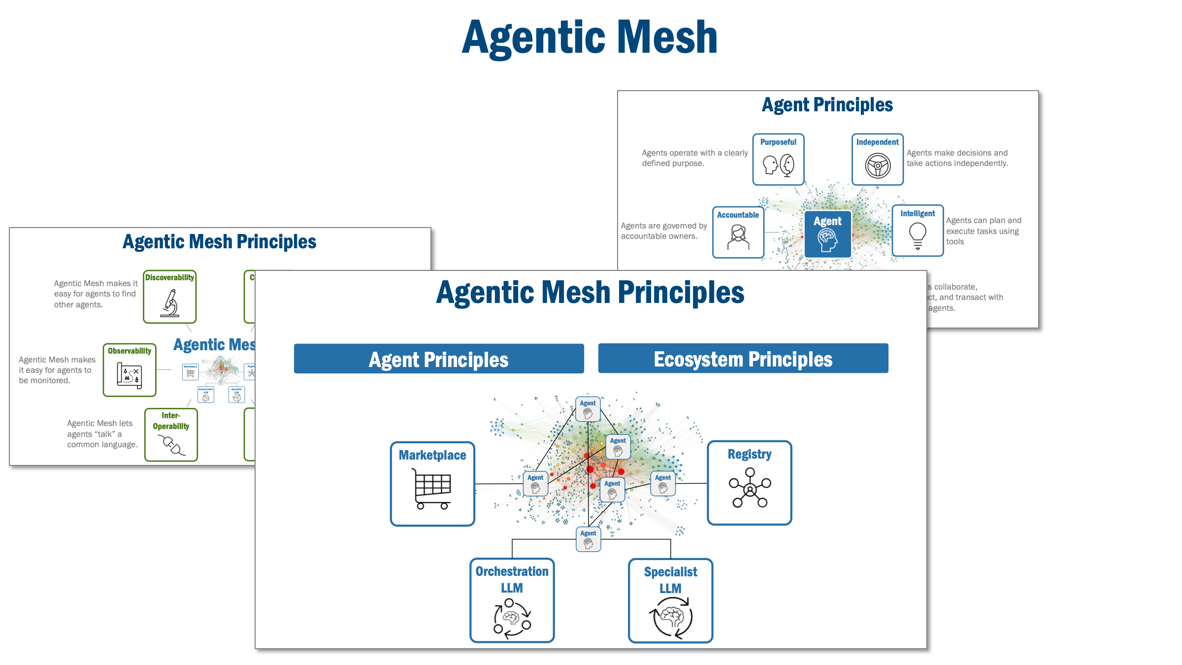
Foundational principles that let autonomous agents find each other, collaborate, interact, and transact in a growing Agentic Mesh…
Originally appeared here:
Agentic Mesh — Principles for an Autonomous Agent Ecosystem
Go Here to Read this Fast! Agentic Mesh — Principles for an Autonomous Agent Ecosystem
Creating data visualizations with Python as alternatives to bar charts, pie charts, and some 3D plots.
Originally appeared here:
3 Triangle-Shaped Chart Ideas as Alternatives to Some Basic Charts
Go Here to Read this Fast! 3 Triangle-Shaped Chart Ideas as Alternatives to Some Basic Charts

Large AI models are resource-intensive. This makes them expensive to use and very expensive to train. A current area of active research, therefore, is about reducing the size of these models while retaining their accuracy. Quantization has emerged as one of the most promising approaches to achieve this goal.
The previous article, Quantizing the Weights of AI Models, illustrated the arithmetics of quantization with numerical examples. It also discussed different types and levels of quantization. This article discusses the next logical step — how to get a quantized model starting from a standard model.
Broadly, there are two approaches to quantizing models:
Since quantization involves replacing high-precision 32-bit floating point weights with 8-bit, 4-bit, or even binary weights, it inevitably results in a loss of model accuracy. The challenge, therefore, is how to quantize models, while minimizing the drop in accuracy.
Because it is an evolving field, researchers and developers often adopt new and innovative approaches. In this article, we discuss two broad techniques:
Conventionally, AI models have been trained using 32-bit floating point weights. There is already a large library of pre-trained models. These trained models can be quantized to lower precision. After quantizing the trained model, one can choose to further fine-tune it using additional data, calibrate the model’s parameters using a small dataset, or just use the quantized model as-is. This is called Post-Training Quantization (PTQ).
There are two broad categories of PTQ:
In this approach, the activations remain in high precision. Only the weights of the trained model are quantized. Weights can be quantized at different granularity levels (per layer, per tensor, etc.). The article Different Approaches to Quantization explains granularity levels.
After quantizing the weights, it is also common to have additional steps like cross-layer equalization. In neural networks, often the weights of different layers and channels can have very different ranges (W_max and W_min). This can cause a loss of information when these weights are quantized using the same quantization parameters. To counter this, it is helpful to modify the weights such that different layers have similar weight ranges. The modification is done in such a way that the output of the activation layers (which the weights feed into) is not affected. This technique is called Cross Layer Equalization. It exploits the scale-equivariance property of the activation function. Nagel et al., in their paper Data-Free Quantization Through Weight Equalization and Bias Correction, discuss cross-layer equalization (Section 4) in detail.
In addition to quantizing the weights as before, for higher accuracy, some methods also quantize the activations. Activations are less sensitive to quantization than weights are. It is empirically observed that activations can be quantized down to 8 bits while retaining almost the same accuracy as 32 bits. However, when the activations are quantized, it is necessary to use additional training data to calibrate the quantization range of the activations.
The advantage is that the training process remains the same and the model doesn’t need to be re-trained. It is thus faster to have a quantized model. There are also many trained 32-bit models to choose from. You start with a trained model and quantize the weights (of the trained model) to any precision — such as 16-bit, 8-bit, or even 1-bit.
The disadvantage is loss of accuracy. The training process optimized the model’s performance based on high-precision weights. So when the weights are quantized to a lower precision, the model is no longer optimized for the new set of quantized weights. Thus, its inference performance takes a hit. Despite the application of various quantization and optimization techniques, the quantized model doesn’t perform as well as the high-precision model. It is also often observed that the PTQ model shows acceptable performance on the training dataset but fails to on new previously unseen data.
To tackle the disadvantages of PTQ, many developers prefer to train the quantized model, sometimes from scratch.
The alternative to PTQ is to train the quantized model. To train a model with low-precision weights, it is necessary to modify the training process to account for the fact that most of the model is now quantized. This is called quantization-aware training (QAT). There are two approaches to doing this:
In many cases, the starting point for QAT is not an untrained model with random weights but rather a pre-trained model. Such approaches are often adopted in extreme quantization situations. The BinaryBERT model discussed later in this series in the article Extreme Quantization: 1-bit AI Models applies a similar approach.
The advantage of QAT is the model performs better because the inference process uses weights of the same precision as was used during the forward pass of the training. The model is trained to perform well on the quantized weights.
The disadvantage is that most models are currently trained using higher precision weights and need to be retrained. This is resource-intensive. It remains to be established if they can match the performance of older higher-precision models in real-world usage. It also remains to be validated if quantized models can be successfully scaled.
QAT, as a practice, has been around for at least a few years. Courbariaux et al, in their 2015 paper titled BinaryConnect: Training Deep Neural Networks with binary weights during propagations, discuss their approach to quantizing Computer Vision neural networks to use binary weights. They quantized weights during the forward pass and unquantized weights during the backpropagation (section 2.3). Jacob et al, then working at Google explain the idea of QAT, in their 2017 paper titled Quantization and Training of Neural Networks for Efficient Integer-Arithmetic-Only Inference (section 3). They do not explicitly use the phrase Quantization Aware Training but call it simulated quantization instead.
The steps below present the important parts of the QAT process, based on the papers referenced earlier. Note that other researchers and developers have adopted variations of these steps, but the overall principle remains the same.
QAT is sometimes referred to as “fake quantization” — it just means that the model training happens using the unquantized weights and the quantized weights are used only for the forward pass. The (latest version of the) unquantized weights are quantized during the forward pass.
The flowchart below gives an overview of the QAT process. The dotted green arrow represents the backpropagation path for updating the model weights while training.
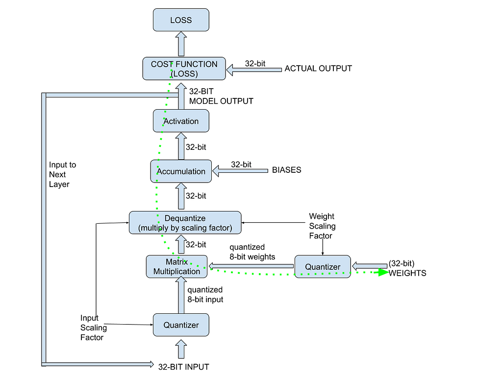
The next section explains some of the finer points involved in backpropagating quantized weights.
It is important to understand how the gradient computation works when using quantized weights. When the forward pass is modified to include the quantizer function, the backward pass must also be modified to include the gradient of this quantizer function. To refresh neural networks and backprop concepts, refer to Understanding Weight Update in Neural Networks by Simon Palma.
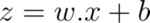
In a regular neural network, given inputs X, weights W, and bias B, the result of the convolution accumulation operation is:
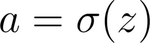
Applying the sigmoid activation function on the convolution gives the model’s output. This is expressed as:
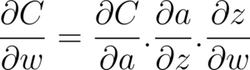
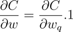
The Cost, C, is a function of the difference between the expected and the actual output. The standard backpropagation process estimates the partial derivative of the cost function, C, with respect to the weights, using the chain rule:
When quantization is involved, the above equation changes to reflect the quantized weight:
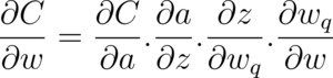
Notice that there is an additional term — which is the partial derivative of the quantized weights with respect to the unquantized weights. Look closely at this (last) partial derivative.
The quantizer function can simplistically be represented as:
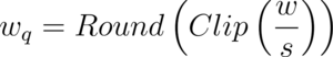
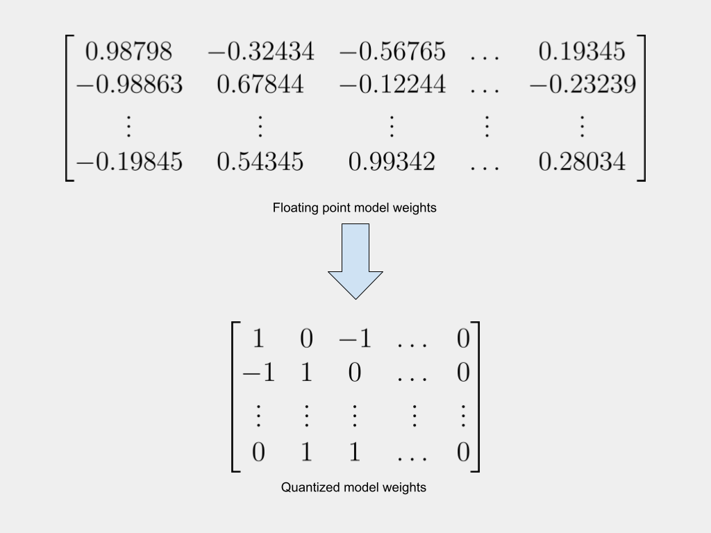
In the expression above, w is the original (unquantized, full-precision) weight, and s is the scaling factor. Recall from Quantizing the Weights of AI Models (or from basic maths) that the graph of the function mapping the floating point weights to the binary weights is a step function, as shown below:
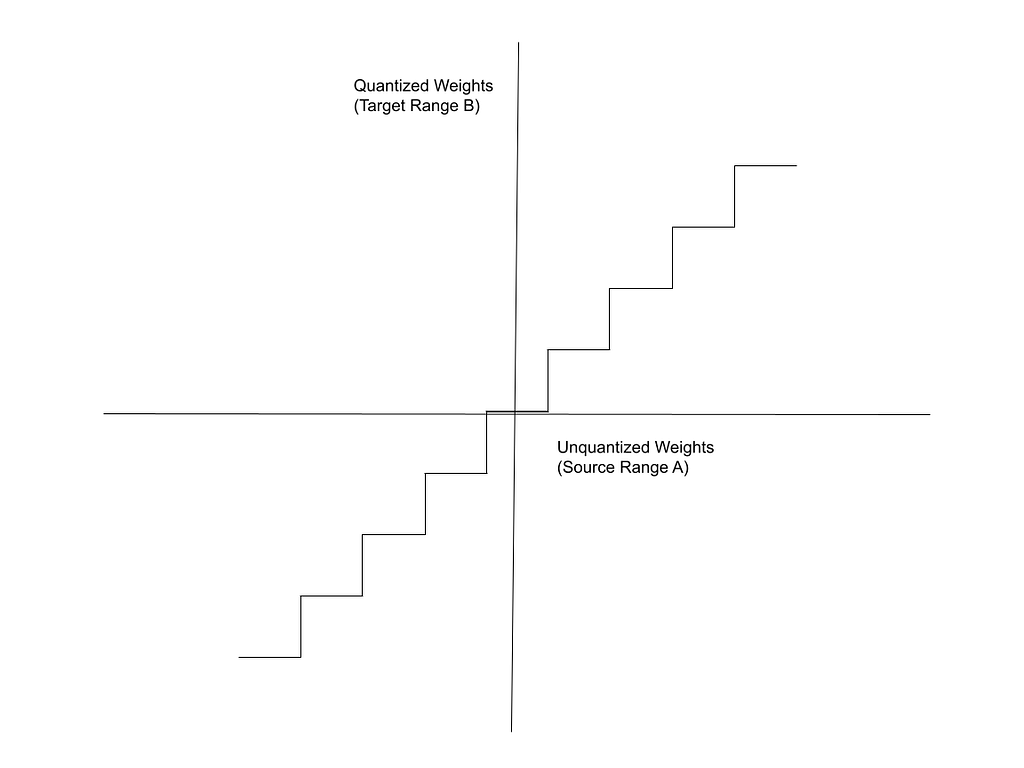
This is the function for which we need the partial derivative. The derivative of the step function is either 0 or undefined — it is undefined at the boundaries between the intervals and 0 everywhere else. To work around this, it is common to use a “Straight-Through Estimator(STE)” for the backprop.
Bengio et al, in their 2013 paper Estimating or Propagating Gradients Through Stochastic Neurons for Conditional Computation, propose the concept of the STE. Huh et al, in their 2023 paper Straightening Out the Straight-Through Estimator: Overcoming Optimization Challenges in Vector Quantized Networks, explain the application of the STE to the derivative of the loss function using the chain rule (Section 2, Equation 7).
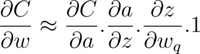
The STE assumes that the gradient with respect to the unquantized weight is essentially equal to the gradient with respect to the quantized weight. In other words, it assumes that within the intervals of the Clip function,
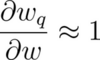
Hence, the derivative of the cost function, C, with respect to the unquantized weights is assumed to be equal to the derivative based on the quantized weights.
Thus, the gradient of the Cost is expressed as:
This is how the Straight Through Estimator enables the gradient computation in the backward pass using quantized weights. After estimating the gradients. The weights for the next iteration are updated as usual (alpha in the expression below refers to the learning rate):
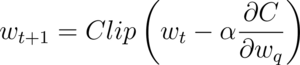
The clip function above is to ensure that the updated (unquantized) weights remain within the boundaries, W_min, and W_max.
Quantizing neural network models makes them accessible enough to run on smaller servers and possibly even edge devices. There are two broad approaches to quantizing models, each with its advantages and disadvantages:
This article discusses both these approaches but focuses on QAT, which is more effective, especially for modern 1-bit quantized LLMs like BitNet and BitNet b1.58. Since 2021, NVIDIA’s TensorRT has included a Quantization Toolkit to perform both QAT and quantized inference with 8-bit model weights. For a more in-depth discussion of the principles of quantizing neural networks, refer to the 2018 whitepaper Quantizing deep convolutional networks for efficient inference, by Krishnamoorthi.
Quantization encompasses a broad range of techniques that can be applied at different levels of precision, different granularities within a network, and in different ways during the training process. The next article, Different Approaches to Quantization, discusses these varied approaches, which are applied in modern implementations like BinaryBERT, BitNet, and BitNet b1.58.
Quantizing Neural Network Models was originally published in Towards Data Science on Medium, where people are continuing the conversation by highlighting and responding to this story.
Originally appeared here:
Quantizing Neural Network Models
A technical walk-through on leveraging multi-modal AI to classify mixed text and image data, including detailed instructions, executable code examples, and tips for effective implementation.

In AI, one of the most exciting areas of growth is multimodal learning, where models process and combine different types of data — such as images and text — to better understand complex scenarios. This approach is particularly useful in real-world applications where information is often split between text and visuals.
Take e-commerce as an example: a product listing might include an image showing what an item looks like and a description providing details about its features. To fully classify and understand the product, both sources of information need to be considered together. Multimodal large language models (LLMs) like Gemini 1.5, Llama 3.2, Phi-3 Vision, and open-source tools such as LlaVA, DocOwl have been developed specifically to handle these types of inputs.
Information from images and text can complement each other in ways that single-modality systems might miss:
If we only process images or text separately, we risk missing critical details. Multimodal models address this challenge by combining both sources during processing, resulting in more accurate and useful outcomes.
This tutorial will guide you through creating a pipeline designed to handle image-text classification. You’ll learn how to process and analyze inputs that combine visual and textual elements, achieving results that are more accurate than those from text-only systems.
If your project involves text-only classification, you might find my other blog post helpful — it focuses specifically on those methods.
Building a Reliable Text Classification Pipeline with LLMs: A Step-by-Step Guide
To successfully build a multimodal image-text classification system, we’ll need three essential components. Here’s a breakdown of each element:
The backbone of this tutorial is a hosted LLM as a service. After experimenting with several options, I found that not all LLMs deliver consistent results, especially when working with structured outputs. Here’s a summary of my experience:
To interface with the LLM and handle multimodal inputs, we’ll use the LangChain library. LangChain is particularly well-suited for this task because it allows us to:
Structured outputs are especially important for classification tasks, as they involve predefined classes that the output must conform to. LangChain ensures this structure is enforced, making it ideal for our use case.
The task we’ll focus on in this tutorial is keyword suggestion for photography-related images. This is a multi-label classification problem, meaning that:
For instance, an input consisting of an image and its description might be classified with keywords like landscape, sunset, and nature. While multiple keywords can apply to a single input, they must be selected from the predefined set of classes.
Now that we have the foundational concepts covered, let’s dive into the implementation. This step-by-step guide will walk you through configuring Gemini 1.5, setting up LangChain, and building a keyword suggestion system for photography-related images.
The first step is to get your Gemini API key, which you can generate in Google AI Studio. Once you have your key, export it to an environment variable called GOOGLE_API_KEY. You can either:
GOOGLE_API_KEY=your_api_key_here
export GOOGLE_API_KEY=your_api_key_here
Next, install the necessary libraries:
pip install langchain-google-genai~=2.0.4 langchain~=0.3.6
Once installed, initialize the client:
import os
from langchain_google_genai import ChatGoogleGenerativeAI

GOOGLE_MODEL_NAME = os.environ.get("GOOGLE_MODEL_NAME", "gemini-1.5-flash-002")

llm_google_client = ChatGoogleGenerativeAI(
    model=GOOGLE_MODEL_NAME,
    temperature=0,
    max_retries=10,
)
To ensure the LLM produces valid, structured results, we use Pydantic to define an output schema. This schema acts as a filter, validating that the categories returned by the model match our predefined list of acceptable values.
from typing import List, Literal
from pydantic import BaseModel, field_validator

def generate_multi_label_classification_model(list_classes: list[str]):
    assert list_classes  # Ensure classes are provided

    class ClassificationOutput(BaseModel):
        category: List[Literal[tuple(list_classes)]]

        @field_validator("category", mode="before")
        def filter_invalid_categories(cls, value):
            if isinstance(value, list):
                return [v for v in value if v in list_classes]
            return []  # Return an empty list if input is invalid

    return ClassificationOutput
Why field_validator Is Needed as a Workaround:
While defining the schema, we encountered a limitation in Gemini 1.5 (and similar LLMs): they do not strictly enforce enums. This means that even though we provide a fixed set of categories, the model might return values outside this set. For example:
Without handling this, the invalid categories could cause errors or degrade the classification’s accuracy. To address this, the field_validator method is used as a workaround. It acts as a filter, ensuring:
This safeguard ensures the model’s results align with the task’s requirements. It is annoying we have to do this but it seems to be a common issue for all LLM providers I tested, if you know of one that handles Enums well let me know please.
Next, bind the schema to the client for structured output handling:
list_classes = [
    "shelter", "mesa", "dune", "cave", "metropolis",
    "reef", "finger", "moss", "pollen", "daisy",
    "fire", "daisies", "tree trunk",  # Add more classes as needed
]

categories_model = generate_multi_label_classification_model(list_classes)
llm_classifier = llm_google_client.with_structured_output(categories_model)
Define the prediction function to send image and text inputs to the LLM:
...
    def predict(self, text: str = None, image_url: str = None) -> list:
        assert text or image_url, "Provide either text or an image URL."

        content = []

        if text:
            content.append({"type": "text", "text": text})

        if image_url:
            image_data = base64.b64encode(httpx.get(image_url).content).decode("utf-8")
            content.append(
                {
                    "type": "image_url",
                    "image_url": {"url": f"data:image/jpeg;base64,{image_data}"},
                }
            )

        prediction = self.llm_classifier.invoke(
            [SystemMessage(content=self.system_prompt), HumanMessage(content=content)]
        )

        return prediction.category
To send image data to the Gemini LLM API, we need to encode the image into a format the model can process. This is where base64 encoding comes into play.
What is Base64?
Base64 is a binary-to-text encoding scheme that converts binary data (like an image) into a text format. This is useful when transmitting data that might otherwise be incompatible with text-based systems, such as APIs. By encoding the image into base64, we can include it as part of the payload when sending data to the LLM.
Finally, run the classifier and see the results. Let’s test it with an example:

classic red and white bus parked beside road
['transportation', 'vehicle', 'road', 'landscape', 'desert', 'rock', 'mountain']
['transportation', 'vehicle', 'road']
As shown, when using both text and image inputs, the results are more relevant to the actual content. With text-only input, the LLM gave correct but incomplete values.

black and white coated dog
Result:
['animal', 'mammal', 'dog', 'pet', 'canine', 'wildlife']
Text Only:
['animal', 'mammal', 'canine', 'dog', 'pet']
Multimodal classification, which combines text and image data, provides a way to create more contextually aware and effective AI systems. In this tutorial, we built a keyword suggestion system using Gemini 1.5 and LangChain, tackling key challenges like structured output handling and encoding image data.
By blending text and visual inputs, we demonstrated how this approach can lead to more accurate and meaningful classifications than using either modality alone. The practical examples highlighted the value of combining data types to better capture the full context of a given scenario.
This tutorial focused on text and image classification, but the principles can be applied to other multimodal setups. Here are some ideas to explore next:
These directions demonstrate the flexibility of multimodal approaches and their potential to address diverse real-world challenges. As multimodal AI evolves, experimenting with various input combinations will open new possibilities for more intelligent and responsive systems.
Full code: llmclassifier/llm_multi_modal_classifier.py
Integrating Text and Images for Smarter Data Classification was originally published in Towards Data Science on Medium, where people are continuing the conversation by highlighting and responding to this story.
Originally appeared here:
Integrating Text and Images for Smarter Data Classification
Go Here to Read this Fast! Integrating Text and Images for Smarter Data Classification


Originally appeared here:
Build cost-effective RAG applications with Binary Embeddings in Amazon Titan Text Embeddings V2, Amazon OpenSearch Serverless, and Amazon Bedrock Knowledge Bases