In this post, we explore a practical, cost-effective approach for incorporating responsible AI guardrails into Amazon Bedrock Batch Inference workflows. Although we use a call center’s transcript summarization as our primary example, the methods we discuss are broadly applicable to a variety of batch inference use cases where ethical considerations and data protection are a top priority.
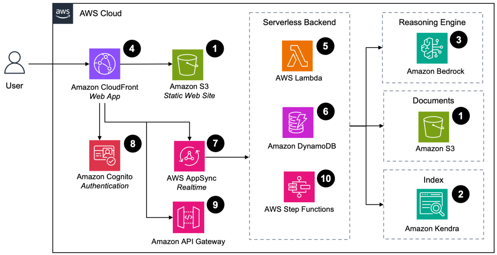
we’re excited to share the journey of the VW—an innovator in the automotive industry and Europe’s largest car maker—to enhance knowledge management by using generative AI, Amazon Bedrock, and Amazon Kendra to devise a solution based on Retrieval Augmented Generation (RAG) that makes internal information more easily accessible by its users. This solution efficiently handles documents that include both text and images, significantly enhancing VW’s knowledge management capabilities within their production domain.
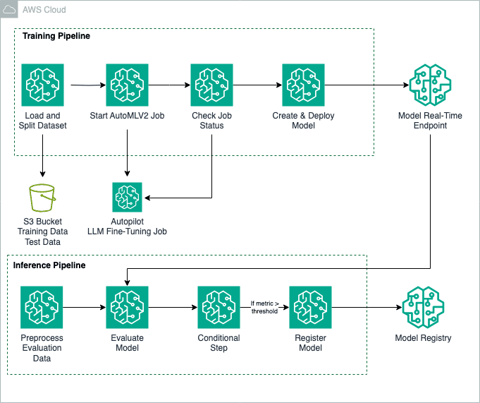
Fine-tuning foundation models (FMs) is a process that involves exposing a pre-trained FM to task-specific data and fine-tuning its parameters. It can then develop a deeper understanding and produce more accurate and relevant outputs for that particular domain. In this post, we show how to use an Amazon SageMaker Autopilot training job with the AutoMLV2 […]
There are a lot of good reasons to get explanations for your model outputs. For example, they could help you find problems with your model, or they just could be a way to provide more transparency to the user, thereby facilitating user trust. This is why, for models like XGBoost, I have regularly applied methods like SHAP to get more insights into my model’s behavior.
Now, with myself more and more dealing with LLM-based ML systems, I wanted to explore ways of explaining LLM models the same way I did with more traditional ML approaches. However, I quickly found myself being stuck because:
SHAP does offer examples for text-based models, but for me, they failed with newer models, as SHAP did not support the embedding layers.
Captum also offers a tutorial for LLM attribution; however, both presented methods also had their very specific drawbacks. Concretely, the perturbation-based method was simply too slow, while the gradient-based method was letting my GPU memory explode and ultimately failed.
After playing with quantization and even spinning up GPU cloud instances with still limited success I had enough I took a step back.
A Similarity-based Approach
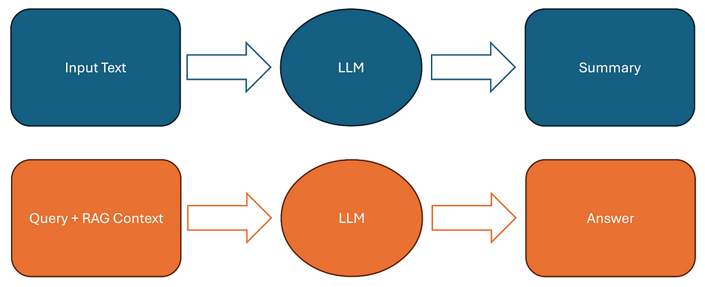
For understanding the approach, let’s first briefly define what we want to achieve. Concretely, we want to identify and highlight sections in our input text (e.g. long text document or RAG context) that are highly relevant to our model output (e.g., a summary or RAG answer).
Typical flow of tasks our explainability method is applicable to. (image created by author)
In case of summarization, our method would have to highlight parts of the original input text that are highly reflected in the summary. In case of a RAG system, our approach would have to highlight document chunks from the RAG context that are showing up in the answer.
Since directly explaining the LLM itself has proven intractable for me, I instead propose to model the relation between model inputs and outputs via a separate text similarity model. Concretely, I implemented the following simple but effective approach:
I split the model inputs and outputs into sentences.
I calculate pairwise similarities between all sentences.
I then normalize the similarity scores using Softmax
After that, I visualize the similarities between input and output sentences in a nice plot
Please, also check out this Github Repository for the full code accompanying this blog post.
from sentence_transformers import SentenceTransformer from nltk.tokenize import sent_tokenize import numpy as np
# Original text truncated for brevity ... text = """This section briefly summarizes the state of the art in the area of semantic segmentation and semantic instance segmentation. As the majority of state-of-the-art techniques in this area are deep learning approaches we will focus on this area. Early deep learning-based approaches that aim at assigning semantic classes to the pixels of an image are based on patch classification. Here the image is decomposed into superpixels in a preprocessing step e.g. by applying the SLIC algorithm [1].
Other approaches are based on so-called Fully Convolutional Neural Networks (FCNs). Here not an image patch but the whole image are taken as input and the output is a two-dimensional feature map that assigns class probabilities to each pixel. Conceptually FCNs are similar to CNNs used for classification but the fully connected layers are usually replaced by transposed convolutions which have learnable parameters and can learn to upsample the extracted features to the final pixel-wise classification result. ..."""
# Define a concise summary that captures the key points summary = "Semantic segmentation has evolved from early patch-based classification approaches using superpixels to more advanced Fully Convolutional Networks (FCNs) that process entire images and output pixel-wise classifications."
# Load the embedding model model = SentenceTransformer('BAAI/bge-small-en')
# Create and print attribution dictionary attributions = { sentence: float(score) for sentence, score in zip(input_sentences, final_scores) }
print("nInput sentences and their attribution scores:") for sentence, score in attributions.items(): print(f"nScore {score:.3f}: {sentence}")
So, as you can see, so far, that is pretty simple. Obviously, we don’t explain the model itself. However, we might be able to get a good sense of relations between input and output sentences for this specific type of tasks (summarization / RAG Q&A). But how does this actually perform and how to visualize the attribution results to make sense of the output?
Evaluation for RAG and Summarization
To visualize the outputs of this approach, I created two visualizations that are suitable for showing the feature attributions or connections between input and output of the LLM, respectively.
These visualizations were generated for a summary of the LLM input that goes as follows:
This section discusses the state of the art in semantic segmentation and instance segmentation, focusing on deep learning approaches. Early patch classification methods use superpixels, while more recent fully convolutional networks (FCNs) predict class probabilities for each pixel. FCNs are similar to CNNs but use transposed convolutions for upsampling. Standard architectures include U-Net and VGG-based FCNs, which are optimized for computational efficiency and feature size. For instance segmentation, proposal-based and instance embedding-based techniques are reviewed, including the use of proposals for instance segmentation and the concept of instance embeddings.
Visualizing the Feature Attributions
For visualizing the feature attributions, my choice was to simply stick to the original representation of the input data as close as possible.
Visualization of sentence-wise feature attribution scores based on color mapping. (image created by author)
Concretely, I simply plot the sentences, including their calculated attribution scores. Therefore, I map the attribution scores to the colors of the respective sentences.
In this case, this shows us some dominant patterns in the summarization and the source sentences that the information might be stemming from. Concretely, the dominance of mentions of FCNs as an architecture variant mentioned in the text, as well as the mention of proposal- and instance embedding-based instance segmentation methods, are clearly highlighted.
In general, this method turned out to work pretty well for easily capturing attributions on the input of a summarization task, as it is very close to the original representation and adds very low clutter to the data. I could imagine also providing such a visualization to the user of a RAG system on demand. Potentially, the outputs could also be further processed to threshold to certain especially relevant chunks; then, this could also be displayed to the user by default to highlight relevant sources.
Again, check out the Github Repository to get the visualization code
Visualizing the Information Flow
Another visualization technique focuses not on the feature attributions, but mostly on the flow of information between input text and summary.
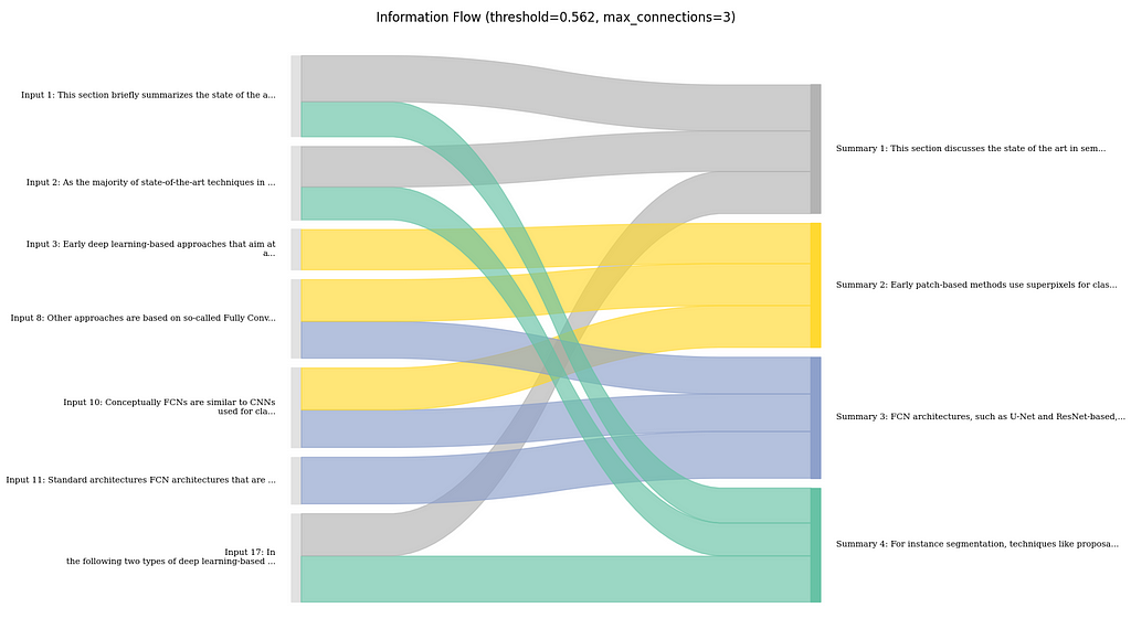
Visualization of the information flow between sentences in Input text and summary as Sankey diagram. (image created by author)
Concretely, what I do here, is to first determine the major connections between input and output sentences based on the attribution scores. I then visualize those connections using a Sankey diagram. Here, the width of the flow connections is the strength of the connection, and the coloring is done based on the sentences in the summary for better traceability.
Here, it shows that the summary mostly follows the order of the text. However, there are few parts where the LLM might have combined information from the beginning and the end of the text, e.g., the summary mentions a focus on deep learning approaches in the first sentence. This is taken from the last sentence of the input text and is clearly shown in the flow chart.
In general, I found this to be useful, especially to get a sense on how much the LLM is aggregating information together from different parts of the input, rather than just copying or rephrasing certain parts. In my opinion, this can also be useful to estimate how much potential for error there is if an output is relying too much on the LLM for making connections between different bits of information.
Possible Extensions and Adaptations
In the code provided on Github I implemented certain extensions of the basic approach shown in the previous sections. Concretely I explored the following:
Use of different aggregations, such as max, for the similarity score. This can make sense as not necessarily the mean similarity to output sentences is relevant. Already one good hit could be relevant for out explanation.
Use of different window sizes, e.g., taking chunks of three sentences to compute similarities. This again makes sense if suspecting that one sentence alone is not enough content to truly capture relatedness of two sentences so a larger context is created.
Use of cross-encoding-based models, such as rerankers. This could be useful as rerankers are more rexplicitely modeling the relatedness of two input documents in one model, being way more sensitive to nuanced language in the two documents. See also my recent post on Towards Data Science.
As said, all this is demoed in the provided Code so make sure to check that out as well.
Conclusion
In general, I found it pretty challenging to find tutorials that truly demonstrate explainability techniques for non-toy scenarios in RAG and summarization. Especially techniques that are useful in “real-time” scenarios, and are thus providing low-latency seemed to be scarce. However, as shown in this post, simple solutions can already give quite nice results when it comes to showing relations between documents and answers in a RAG use case. I will definitely explore this further and see how I can probably use that in RAG production scenarios, as providing traceable outputs to the users has proven invaluable to me. If you are interested in the topic and want to get more content in this style, follow me here on Medium and on LinkedIn.
Taking the first step towards mastering a new topic is always a bit daunting—sometimes it’s even very daunting! It doesn’t matter if you’re learning about algorithms for the first time, dipping your toes into the exciting world of LLMs, or have just been tasked with revamping your team’s data stack: taking on a challenge with little or no prior experience requires nontrivial amounts of courage and grit.
The calm and nuanced perspective of more seasoned practitioners can go a long way, too — which is where our authors excel. This week, we’ve gathered some of our standout recent contributions that are tailored specifically to the needs of early-stage learners attempting to expand their skill set. Let’s roll up our sleeves and get started!
From Parallel Computing Principles to Programming for CPU and GPU Architectures For freshly minted data scientists and ML engineers, few areas are more crucial to understand than memory fundamentals and parallel execution. Shreya Shukla’s thorough and accessible guide is the perfect resource to get a firm footing in this topic, focusing on how to write code for both CPU and GPU architectures to accomplish fundamental tasks like vector-matrix multiplication.
Multimodal Models — LLMs That Can See and Hear If you’re feeling confident in your knowledge of LLM basics, why not take the next step and explore multimodal models, which can take in (and in some cases, generate) multiple forms of data—from images to code and audio? Shaw Talebi’s primer, the first part of a new series, offers a solid foundation from which to build your practical know-how.
Boosting Algorithms in Machine Learning, Part II: Gradient Boosting Whether you’ve only recently started your ML journey or have been at it for so long that a refresher might be useful, it’s never a bad idea to firm up your knowledge of the basics. Gurjinder Kaur’s ongoing exploration of boosting algorithms is a great case in point, presenting accessible, easy-to-digest breakdowns of some of the most powerful models out there—in this case, gradient boosting.
NLP Illustrated, Part 1: Text Encoding Another new project we’re thrilled to share with our readers? Shreya Rao’s just-launched series of illustrated guides to core concepts in natural language processing, the very technology powering many of the fancy chatbots and AI apps that have made a splash in recent years. Part one zooms in on an essential step in just about any NLP workflow: turning textual data into numerical inputs via text encoding.
Decoding One-Hot Encoding: A Beginner’s Guide to Categorical Data If you’re looking to learn about another form of data transformation, don’t miss Vyacheslav Efimov’s clear and concise introduction to one-hot encoding, “one of the most fundamental techniques used for data preprocessing,” turning categorical features into numerical vectors.
Excel Spreadsheets Are Dead for Big Data. Companies Need More Python Instead. One type of transition that is often even more difficult than learning a new topic is switching to a new tool or workflow—especially when the one you’re moving away from fits squarely within your comfort zone. As Ari Joury, PhD explains, however, sometimes a temporary sacrifice of speed and ease of use is worth it, as in the case of adopting Python-based data tools instead of Excel spreadsheets.
Ready to venture out into other topics and challenges this week? We hope so—we’ve published some excellent articles recently on LLM apps, Python-generated art, AI ethics, and more:
Thank you for supporting the work of our authors! As we mentioned above, we love publishing articles from new authors, so if you’ve recently written an interesting project walkthrough, tutorial, or theoretical reflection on any of our core topics, don’t hesitate to share it with us.
An open-source initiative to help you deploy generative search based on your local files and self-hosted (Mistral, Llama 3.x) or commercial LLM models (GPT4, GPT4o, etc.)
I have previously written about building your own simple generative search, as well as on the VerifAI project on Towards Data Science. However, there has been a major update worth revisiting. Initially, VerifAI was developed as a biomedical generative search with referenced and AI-verified answers. This version is still available, and we now call it VerifAI BioMed. It can be accessed here: https://app.verifai-project.com/.
The major update, however, is that you can now index your local files and turn them into your own generative search engine (or productivity engine, as some refer to these systems based on GenAI). It can serve also as an enterprise or organizational generative search. We call this version VerifAI Core, as it serves as the foundation for the other version. In this article, we will explore how you can in a few simple steps, deploy it and start using it. Given that it has been written in Python, it can be run on any kind of operating system.
Architecture
The best way to describe a generative search engine is by breaking it down into three parts (or components, in our case):
Indexing
Retrieval-Augmented Generation (RAG) Method
VerifAI contains an additional component, which is a verification engine, on top of the usual generative search capabilities
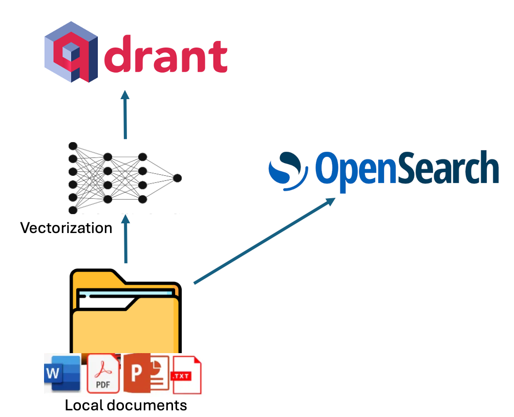
Indexing in VerifAI can be done by pointing its indexer script to a local folder containing files such as PDF, MS Word, PowerPoint, Text, or Markdown (.md). The script reads and indexes these files. Indexing is performed in dual mode, utilizing both lexical and semantic indexing.
For lexical indexing, VerifAI uses OpenSearch. For semantic indexing, it vectorizes chunks of the documents using an embedding model specified in the configuration file (models from Hugging Face are supported) and then stores these vectors in Qdrant. A visual representation of this process is shown in the diagram below.
Architecture of indexing (diagram by author)
When it comes to answering questions using VerifAI, the method is somewhat complex. User questions, written in natural language, undergo preprocessing (e.g., stopwords are excluded) and are then transformed into queries.
For OpenSearch, only lexical processing is performed (e.g., excluding stopwords), and the most relevant documents are retrieved. For Qdrant, the query is transformed into embeddings using the same model that was used to embed document chunks when they were stored in Qdrant. These embeddings are then used to query Qdrant, retrieving the most similar documents based on dot product similarity. The dot product is employed because it accounts for both the angle and magnitude of the vectors.
Finally, the results from the two engines must be merged. This is done by normalizing the retrieval scores from each engine to values between 0 and 1 (achieved by dividing each score by the highest score from its respective engine). Scores corresponding to the same document are then added together and sorted by their combined score in descending order.
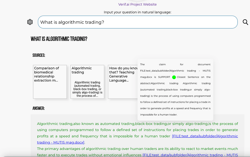
Using the retrieved documents, a prompt is built. The prompt contains instructions, the top documents, and the user’s question. This prompt is then passed to the large language model of choice (which can be specified in the configuration file, or, if no model is set, defaults to our locally deployed fine-tuned version of Mistral). Finally, a verification model is applied to ensure there are no hallucinations, and the answer is presented to the user through the GUI. The schematic of this process is shown in the image below.
When installing VerifAI Search, it is recommended to start by creating a clean Python environment. I have tested it with Python 3.6, but it should work with most Python 3 versions. However, Python 3.10+ may encounter compatibility issues with certain dependencies.
To create a Python environment, you can use the venv library as follows:
After activating the environment, you can install the required libraries. The requirements file is located in theverifAI/backenddirectory. You can run the following command to install all the dependencies:
pip install -r requirements.txt
Configuring system
The next step is configuring VerifAI and its interactions with other tools. This can be done either by setting environment variables directly or by using an environment file (the preferred option).
An example of an environment file for VerifAI is provided in the backend folder as .env.local.example. You can rename this file to .env, and the VerifAI backend will automatically read it. The file structure is as follows:
Some of the variables are quite straightforward. The first Secret key and Algorithm are used for communication between the frontend and the backend.
Then there are variables configuring access to the PostgreSQL database. It needs the database name (DBNAME), username, password, and host address where the database is located. In our case, it is on localhost, on the docker image.
The next section is the configuration of OpenSearch access. There is IP (localhost in our case again), username, password, port number (default port is 9200), and variable defining whether to use SSL.
A similar configuration section has Qdrant, just for Qdrant, we use an API key, which has to be here defined.
The next section defined the generative model. VerifAI uses the OpenAI python library, which became the industry standard, and allows it to use both OpenAI API, Azure API, and user deployments via vLLM, OLlama, or Nvidia NIMs. The user needs to define the path to the interface, API key, and model deployment name that will be used. We are soon adding support where users can modify or change the prompt that is used for generation. In case no path to an interface is provided and no key, the model will download the Mistral 7B model, with the QLoRA adapter that we have fine-tuned, and deploy it locally. However, in case you do not have enough GPU RAM, or RAM in general, this may fail, or work terribly slowly.
You can set also MAX_CONTEXT_LENGTH, in this case it is set to 128,000 tokens, as that is context size of GPT4o. The context length variable is used to build context. Generally, it is built by putting in instruction about answering question factually, with references, and then providing retrieved relevant documents and question. However, documents can be large, and exceed context length. If this happens, the documents are splitted in chunks and top n chunks that fit into the context size will be used to context.
The next part contains the HuggingFace name of the model that is used for embeddings of documents in Qdrant. Finally, there are names of indexes both in OpenSearch (INDEX_NAME_LEXICAL) and Qdrant (INDEX_NAME_SEMANTIC).
As we previously said, VerifAI has a component that verifies whether the generated claim is based on the provided and referenced document. However, this can be turned on or off, as for some use-cases this functionality is not needed. One can turn this off by setting USE_VERIFICATION to False.
Installing datastores
The final step of the installation is to run the install_datastores.py file. Before running this file, you need to install Docker and ensure that the Docker daemon is running. As this file reads configuration for setting up the user names, passwords, or API keys for the tools it is installing, it is necessary to first make a configuration file. This is explained in the next section.
This script sets up the necessary components, including OpenSearch, Qdrant, and PostgreSQL, and creates a database in PostgreSQL.
python install_datastores.py
Note that this script installs Qdrant and OpenSearch without SSL certificates, and the following instructions assume SSL is not required. If you need SSL for a production environment, you will need to configure it manually.
Also, note that we are talking about local installation on docker here. If you already have Qdrant and OpenSearch deployed, you can simply update the configuration file to point to those instances.
Indexing files
This configuration is used by both the indexing method and the backend service. Therefore, it must be completed before indexing. Once the configuration is set up, you can run the indexing process by pointing index_files.py to the folder containing the files to be indexed:
We have included a folder called test_data in the repository, which contains several test files (primarily my papers and other past writings). You can replace these files with your own and run the following:
python index_files.py test_data
This would run indexing over all files in that folder and its subfolders. Once finished, one can run VerifAI services for backend and frontend.
Running the generative search
The backend of VerifAI can be run simply by running:
python main.py
This will start the FastAPI service that would act as a backend, and pass requests to OpenSearch, and Qdrant to retrieve relevant files for given queries and to the deployment of LLM for generating answers, as well as utilize the local model for claim verification.
Frontend is a folder called client-gui/verifai-ui and is written in React.js, and therefore would need a local installation of Node.js, and npm. Then you can simply install dependencies by running npm install and run the front end by running npm start:
cd ..
cd client-gui/verifai-ui
npm install
npm start
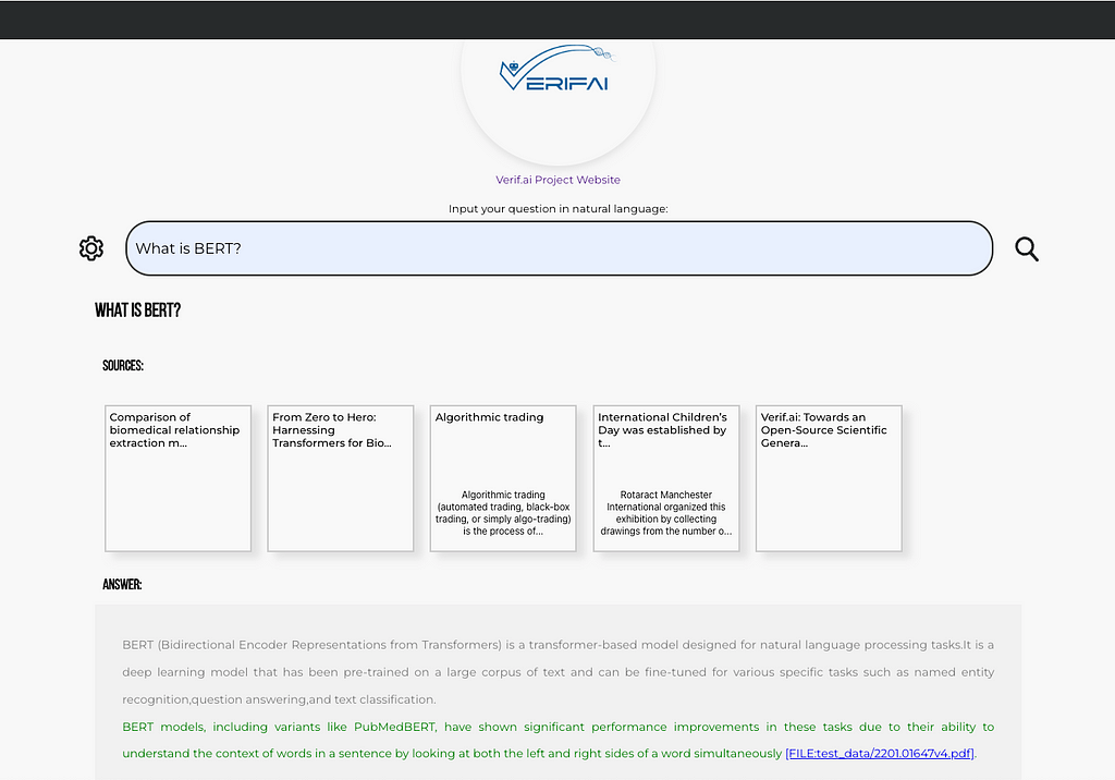
Finally, things should look somehow like this:
One of the example questions, with verification turned on (note text in green) and reference to the file, which can be downloaded (screenshot by author)Screenshot showcasing tooltip of the verified claim, with the most similar sentence from the article presented (screenshot by author)
Contributing and future direction
So far, VerifAI has been started with the help of funding from the Next Generation Internet Search project as a subgrant of the European Union. It was started as a collaboration between The Institute for Artificial Intelligence Research and Development of Serbia and Bayer A.G.. The first version has been developed as a generative search engine for biomedicine. This product will continue to run at https://app.verifai-project.com/. However, lately, we decided to expand the project, so it can truly become an open-source generative search with verifiable answers for any files, that can be leveraged openly by different enterprises, small and medium companies, non-governmental organizations, or governments. These modifications have been developed by Natasa Radmilovic and me voluntarily (huge shout out to Natasa!).
However, given this is an open-source project, available on GitHub (https://github.com/nikolamilosevic86/verifAI), we are welcoming contributions by anyone, via pull requests, bug reports, feature requests, discussions, or anything else you can contribute with (feel free to get in touch — for both BioMed and Core (document generative search, as described here) versions website will remain the same — https://verifai-project.com). So we welcome you to contribute, start our project, and follow us in the future.
Data is booming. It comes in vast volumes and variety and this explosion comes with a plethora of job opportunities too. Is it worth switching to a data career now? My honest opinion: absolutely!
It is worth mentioning that this article comes from an Electrical and Electronic Engineer graduate who went all the way and spent almost 8 years in academia learning about the Energy sector (and when I say all the way, I mean from a bachelor degree to a PhD and postdoc). Even though that’s also a high demand career in the job market, I decided to switch to a data engineer path instead.
I constantly come across posts in forums and blogs where people from different disciplines ask about how to switch to a career in data. So this article will take you through my journey, and how an engineering graduate has nothing to worry about the transition to this new field. I’ll go through the market for data jobs, my story, and the skills that engineers have (whether it’s electrical, mechanical, electronic etc.) that equip them well for this fast moving field.
Generative AI image that I got when I wrote my article title in ChatGPT. Impressive, isn’t it?
Necessity for Data Professionals
As technology continues to advance exponentially (IoT devices, AI, web services etc.) so does the amount of data generated every day. The result from this? The need for AI and Data professionals is currently at an all time high and I think it is only going to get higher. It’s currently at a level that the demand for these professionals severely outgrows supply and new job listings are popping out every day.
According to Dice Tech Job Report, positions like Data Engineers and Data Scientists are amongst the fastest growing tech occupations. The reason being that companies have finally come to the realization that, with data, you can unlock unlimited business insights which can reveal their product’s strengths and weaknesses. That is, if analyzed the correct way.
So what does this mean for the future data professionals looking for a job? The following should be true, at least for the next few years:
Unlimited job listings: According to a recent report by LinkedIn, job postings for AI roles have surged by 119% over the past two years. Similarly, data engineering positions have seen a 98% increase. This highlights the urgency of companies to hire these kind of professionals.
High salary potential: When demand exceeds supply, it immediately leads to higher salaries. These are fundamental laws of economics. Data professionals are now in an era where they have multiple options for a job since companies acknowledge the value they bring to their company.
Multiple industry opportunities: Take my case for example. I worked in data for energy, retail and finance sectors. I consider myself data agnostic, since I am now able to choose from opportunities across a relatively wide range of industries.
Future job growth: As mentioned before, the need for these professionals is only going to get higher since data comes in all shapes and sizes and there is a need for people that know how to handle it.
Switching from another Engineering principle to Data
So here comes the million dollar question: How can an Engineer, whether that is mechanical, electronic, electrical, civil etc. switch to a career in data? Great question.
Is it easy? No. Is it worth it? Definitely. There’s no correct answer for this question. However, I can tell you my experiences and you can judge on your own. I can also tell you the similarities I found between my engineering degree and what I’m doing now. So let’s start.
A brief story of how I switched to data engineering:
Years 2020–2022
The year is 2020 and I’m about to finish my PhD. Confused about my options and what I can do after a long 4-year PhD (and with a severe imposter syndrome too), I chose the safe path of academia and a postdoc position at a Research and Development center.
Imposter syndrome is, funny enough, very common to PhD graduates. It is defined as “The persistent inability to believe that one’s success is deserved or has been legitimately achieved as a result of one’s own efforts or skills”. Image Source: DALL-E.
Whilst working there, I realized that I need to get out of academia. I no longer had the strength to read more papers, proposals or, even more so, write journal and conference papers to showcase my work. I did all those — I had enough. I had like 7–8 journal/conference papers that got published from my PhD and I didn’t really like the fact that this is the only way to showcase my work. So, I started looking for a job in the industry.
In 2021, I managed to get a job in energy consulting. And guess what? More reports, more papers and even better, PowerPoint slides! I felt like my engineering days were behind me and that I could literally do nothing useful. After a short stint at that position, I started looking for jobs again. Something with technical challenges and meaning that got my brain working. This is when I started looking for data professions where I could use the skills that I acquired throughout my career. Also, this was the time that I got the most rejections in my life!
Coming from very successful bachelor and PhD degrees, I couldn’t understand why my skills were not suited for a data position. I was applying to data engineer, analyst and scientist positions but all I received was an automated reply like “Unfortunately we can’t move forward with your application”
That’s when I started applying to literally everywhere. So if you are reading this because you can’t make the switch, believe me. I get you.
Years 2022–2023
So, I started applying everywhere to anything that even relates to data. Even to positions that I didn’t have any of the job description skills. That’s where the magic happened.
I got an interview from a company in the retail sector for the position of “Commercial Intelligence Executive”. Do you know what this position is about? No? That’s right, I didn’t either. All I saw in the job description was that it required 3–5 years of experience in Data Science. So I thought, this has something to do with data, so why not. I got the job and started working there. Turns out that “Commercial Intelligence” was a job description that was basically business intelligence for the commercial department. Lucky me, it was spot on. It gave me the opportunity to start experimenting with business intelligence.
Business Intelligence (BI) is defined as “The technical infrastructure that collects, stores and analyzes company data”. Photo by Carlos Muza on Unsplash.
In that position, I used Power BI at first, since the role was about building reports and dashboards. Then, I was hungry for more. I was fortunate that my manager was amazing so he/she trusted me to do whatever I wanted with data. And so I did.
Before I knew it, my engineering skills were back. All the problem solving skills that I got throughout the years, the bug for solving challenges and the exposure to different programming languages started connecting with each other. I started building automations in Power BI, then extended this to writing SQL to automate more things and then building data pipelines using Python. In 1 year’s time, I had all my processes pretty much automated and I knew that I had the technical capability to take on more challenging and technically intensive problems. I built incredible dashboards that brought useful insights to the business owners and that felt incredible.
This was the lightbulb moment. That this career, no matter what the data is about, was what I was looking for.
Years 2023-present
After one and a half years at the company, I knew it was time to go for something more technically challenging than just business intelligence. That’s when an opportunity turned out for me for a data engineer position and I took it.
For the past one and a half years I’ve been working in the finance sector as a data engineer. I expanded my knowledge to more things such as AI, real-time streaming data pipelines, APIs, automations and so much more. Job opportunities are coming up all the time and I feel fortunate that I have made this switch, and I couldn’t recommend it enough. Was it challenging? I’ll say that the only challenging part in both BI and data engineering positions was the first 3 months until I got to know the tools we use and the environments. My engineering expertise equipped me well to deal with different problems with excitement and do amazing things. I wouldn’t change my degree for anything else. Not even for a Computer Science degree. How did my engineering degree help throughout this transition? This is discussed in the next section.
How Engineering equips you with skills that help in a data career
So if you’ve read this far, you must be wondering: How is my engineering degree preparing me for a career in data? This guy has told me nothing about this. You are right, let’s get into it.
Engineering degrees are important, not because of the discipline but the way that they structure the brains of those they study it. This is my personal opinion, but going through my engineering degrees they have exposed me to so many things and have prepared me to solve problems in every single bit that I feel much more confident now. But let’s get to the specifics. These are some key engineering skills that I see similarities and I get to use at my data role every single day:
Programming: As an electrical and electronics engineer, I got exposure to multiple programming languages throughout my degrees. I used assembly language, Java, VHDL, C and Matlab. Likewise, I think other engineering disciplines do the same thing since programming is a way to perform simulations in engineering. Even though I haven’t used Python or SQL during my degrees, it was a seamless transition to these two, after getting exposed to so many things. I would even say enjoyable, since I used to hate coding during my bachelor degree, but now I love it. It probably was a matter of tight deadlines and stress from so many things at the same time.
Problem Solving: I get to solve problems every day but as my first university lecturer said to us at the very first day at the university, “Google is your friend”. If you have a knack for solving problems, and you have been exposed to the way engineering projects are handed out at universities (where they basically give you a one paragraph description for the project and expect a product by the end of the week), believe me you can solve data problems. You have been through enough preparation.
Math and Statistics: Engineering students get through intense mathematics such as linear algebra, calculus, statistics and others that can make you understand machine learning in a smooth transition. It’s a bit difficult to grasp at first because it’s a new territory but you’ll get the hang of it.
Black Box Problems: I don’t even know if this is a formal definition but I consider “Black Box” problems to be the ones that are extremely difficult to solve, we’ve been using them, they work, but not a lot of people actually know what’s happening in the background. In data, the “Black Box Problem” is AI. It’s hot, it works and it’s amazing but no one really knows what’s happening in the background. Similarly, engineering disciplines have their own “Black Box” problems. Sure, AI is difficult but have you tried understanding the power network problem? That’s no walk in the park.
Modelling and Simulations: Every engineer student has been doing modelling and simulations and that’s nothing different from ML models and data models.
Data Processing and Analytics: As an engineer student in my bachelor and PhD degrees I did a lot of data processing, transformation and analytics from oscilloscope files, sensor files and smart devices that had millions of rows of data. These are examples of data pipelines as we call them in the data industry. I didn’t really know at the time though that this was the name for it. When I got to do it in a corporate environment, these skills were transferrable and helped so much.
Automations: Engineers hate repeated procedures. If there’s a way to automate something, they will do it. This is the mindset that a data engineer needs. I carried this mindset to my data engineer position and it helps a lot since I spend a lot of time automating stuff in my day to day.
Presenting and explaining to non-technical people: One very common thing I was doing in my PhD was explaining my project to non-technical people so that they can understand what I’m doing. This happens a lot in data. You prepare a lot of analysis for business people so you have to be able to explain it too.
All the above help me every single day in my data engineer position. Can you see the transferrable skills now?
So, is it a happy ending?
Whilst I don’t want to encourage all the engineering disciplines to jump into a data position, I still think that all engineers are useful, I wanted to write this article to encourage the people that want to do the switch. There’s so much rejection nowadays but at the same time opportunities. All you need is the right opportunity and then magic will follow since you will be able to exploit your skills. The important thing is to keep trying.
Unlike SOTA PEFT methods, which focus on modifying the model weights or input, the ReFT technique is based on a previously proposed distributed interchange intervention (DII) method. The DII method first projects the embedding from the deep learning model to a lower dimension subspace and then interferes through the subspace for fine-tuning purposes.
In the following, we’ll first walk the readers through SOTA fine-tuning PEFT algorithms such as LoRA, prompt tuning, and prefix tuning; then we’ll discuss the original DII method to provide a better context for understanding; lastly, we’ll discuss the ReFT technique and present the results from the paper.
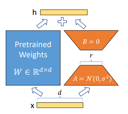
Proposed in 2021, LoRA has become one of the most successful techniques for fine-tuning LLMs and diffusion models (e.g., Time-varying LoRA) due to its simplicity and generalization ability. The idea is simple: instead of fine-tuning the original weight parameters for each layer, the LoRA technique adds two low-rank matrices and only finetunes the low-rank matrices. The trainable parameters could be reduced to less than 0.3% during fine-tuning of the whole network, which significantly speeds up the learning process and minimizes the GPU memory.
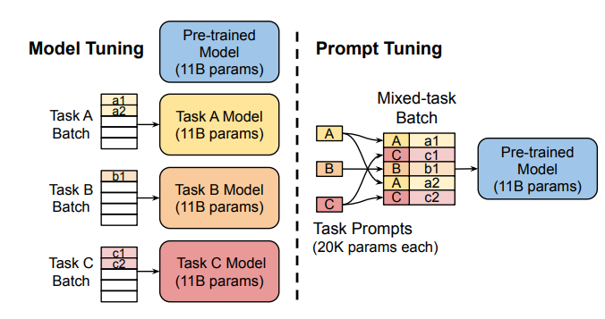
Instead of changing the pre-trained model’s inner layers, the Prompt Tuning technique proposed to use “soft prompts,” a learnable task-specific prompt embedding as a prefix. Given mixed-task batch prompts, the model could efficiently perform multi-task prediction without extra task-specific model copy (as against the Model Tuning in the following left sub-figure).
To provide universality for prompt tuning models at scales (e.g., over 10B parameters), Prefix Tuning (P-Tuning v2) proposed to prefix trainable prompt embeddings at different layers, which allows learning task-specific information at various scales.
Among all these PEFT techniques, LoRA is the most widely used in fine-tuning LLMs for its robustness and efficiency. A detailed empirical analysis can be found in this paper.
Distributed Interchange Intervention (DII)
Causal abstraction is a robust artificial intelligence framework that uses the intervention between a causal model (a high-level model) and a neural network model (or a low-level model) to induce alignment estimation. If there exists an alignment between the two models, we know the underlying mechanisms between the causal model and the NN are the same. The approach of discovering the underlying alignment by intervention is called interchange intervention (II), which is intuitively explained in this lecture video.
However, classical causal abstraction uses brute force to search through all possible alignments of model states, which is less optimal. A Distributed Interchange Intervention (DII) system first projects high-level and low-level models to sub-spaces through a series of orthogonal projections and then produces an intervened model using certain rotation operations. A fascinating intervention experiment on vision models can be found here.
More specifically, the DII could be written as the following:
Where R is a low-rank matrix with orthogonal rows, indicating orthogonal projections; b and s are two different representations encoded by the model from two different inputs; the intervention will happen on the low-rank space, e.g., the space that contains Rs and Rb; the projection matrix R will be further learnt by distributed alignment search (DAS), which optimizes towards “the subspace that would maximize the probability of expected counterfactual output after intervention.”
ReFT — Representation Fintuning
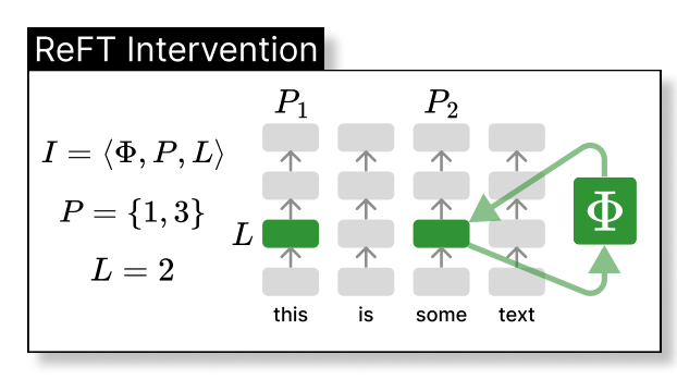
Thus, the ReFT technique could be seen as the intervention of the model’s hidden representation in a lower dimension space, as illustrated below, where phi is the intervention and directly applied to the hidden representation at layer L and position P:
Where h is the hidden representation, (Rs = Wh + b) is the learnt protected source, which edits the representation h in the projected low-dimension space spanned by R. Now, we can illustrate the LoReFT in the original deep neural network layer below.
When fine-tuning on an LLM, the parameters of the LM are kept frozen while only the parameters of the projection phi={R, W, b} are trained.
Experiments
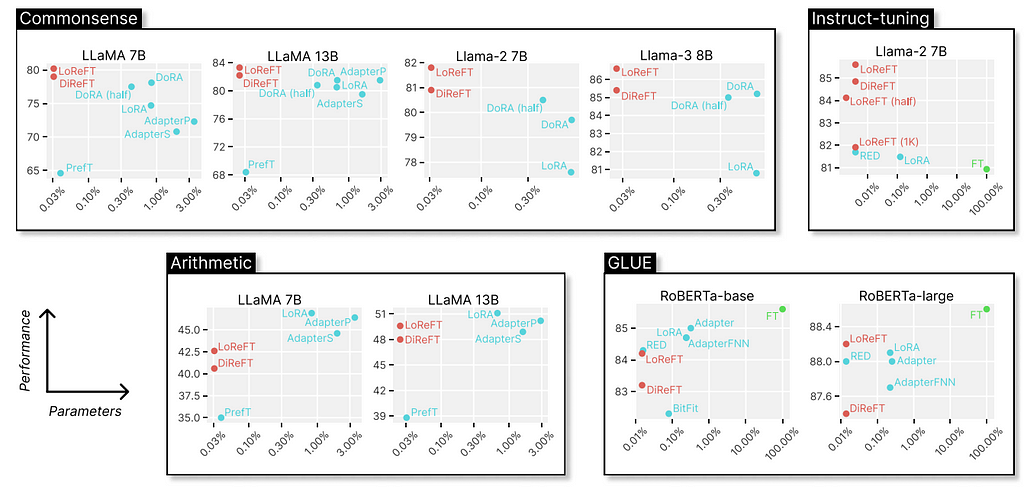
The original paper shows experiments comparing the LoReFT (and other techniques from the ReFT family) to full fine-tuning (FT), LoRA, Prefix-tuning, etc., on four types of benchmarks: common-sense reasoning, arithmetic reasoning, instruction following, and natural language understanding. We can see that, compared to LoRA, the ReFT techniques further reduce the parameters by at least 90% while achieving higher performance by a large margin.
Why is ReFT so fascinating? Firstly, the technique provides convincing results with Llama-family models on various benchmarks outperforming the SOTA fine-tuning methods. Secondly, the technique is deeply rooted in the causal abstraction algorithm, which offers further ground for model interpretation, especially from the hidden representation’s perspective. As mentioned in the original paper, ReFT shows that “a linear subspace distributed across a set of neurons can achieve generalized control over a vast number of tasks,” which might further open doors for helping us better understand large language models.
References
Wu Z, Arora A, Wang Z, Geiger A, Jurafsky D, Manning CD, Potts C. Reft: Representation finetuning for language models. arXiv preprint arXiv:2404.03592. 2024 Apr 4.
Hu EJ, Shen Y, Wallis P, Allen-Zhu Z, Li Y, Wang S, Wang L, Chen W. Lora: Low-rank adaptation of large language models. arXiv preprint arXiv:2106.09685. 2021 Jun 17.
Zhuang Z, Zhang Y, Wang X, Lu J, Wei Y, Zhang Y. Time-Varying LoRA: Towards Effective Cross-Domain Fine-Tuning of Diffusion Models. In The Thirty-eighth Annual Conference on Neural Information Processing Systems 2024.
Liu X, Ji K, Fu Y, Tam WL, Du Z, Yang Z, Tang J. P-tuning v2: Prompt tuning can be comparable to fine-tuning universally across scales and tasks. arXiv preprint arXiv:2110.07602. 2021 Oct 14.
Geiger A, Wu Z, Potts C, Icard T, Goodman N. Finding alignments between interpretable causal variables and distributed neural representations. InCausal Learning and Reasoning 2024 Mar 15 (pp. 160–187). PMLR.
Lester B, Al-Rfou R, Constant N. The power of scale for parameter-efficient prompt tuning. arXiv preprint arXiv:2104.08691. 2021 Apr 18.
Pu G, Jain A, Yin J, Kaplan R. Empirical analysis of the strengths and weaknesses of PEFT techniques for LLMs. arXiv preprint arXiv:2304.14999. 2023 Apr 28.
Is ReFT All We Needed? was originally published in Towards Data Science on Medium, where people are continuing the conversation by highlighting and responding to this story.
A High-Level Framework for Building a CBM System with Strategic Impact
Image created by the author using Canva
Imagine if your customer data could tell a story — one that drove key decisions, optimized pricing, and forecast future revenue with accuracy.
As a data scientist, I have spent a large part of my career designing and building customer base management (CBM) systems. These are systems that monitor and predict anything from customer churn and customer price elasticity to recommending the products customers are most likely to buy.
I have witnessed how CBM systems have been successfully adopted by organizations, and enabled them to execute their strategy through effective pricing, improved retention and more targeted sales activities. Combining forecasting with the visual effect of dashboards, CBM systems can provide an effective way for managers to communicate with executive leadership. This enhances decision-making and helps leaders better understand the consequences of their actions, particularly regarding the customer base and projected future revenues from that base.
In this article we will explore both the foundational components of a CBM system, as well as the more advanced features that really ramp up the value generation. By the end of this guide, you’ll have a clear understanding of the key components of a CBM system and how advanced modules can enhance these foundations to give your company a competitive edge.
The Foundation of a Strong CBM System
Image created by the author using Canva
The three main foundational components of a CBM systems are:
ELT (extract-load-transform)
Basic Churn Modelling
Dashboards
With these three elements in place, managers are afforded a basic understanding of churn, a visual understanding of the data, and furthermore it allows them to communicate any findings to the leadership and other stakeholders. Below we detail each of these components in depth.
ELT — Getting the Data
Extract-Load-Transform, ELT for short, is the first and most critical part of a customer base management system. This is the component that feeds the system with data, and is often the first component to be built when creating a CBM system. To get started, you will typically interact with some kind of data platform where most of the rudimentary data manipulation has already been performed (in this case you are technically only required to do the “load” and “transform”), but sometimes you need get directly from source systems as well and “extract” the data.
Irrespective of where the data comes from, it needs to be loaded into your system and transformed into a format that is easy to input into the machine learning models you are using. You will also likely need to transform the data into formats that makes it easier to make dashboards from the data. For some dashboards it might also be necessary to pre-aggregate a lot of data in smaller tables to improve query and plotting performance.
It is easy to see that if there are mistakes in the ELT process, or if there are errors in the incoming data, this has the potential to severely affect the CBM system. Since everything in the system is based on this incoming data, extra care needs to be taken to ensure accuracy and alignment with business rules.
I have seen multiple times where the ELT process has failed and led to mistakes in the churn predictions and dashboard. One way to monitor the consistency of the data coming into the system is to keep records of the distribution of each variable and track that distribution over time. In case of radical changes to the distribution you can then quickly check whether something is going wrong with the logic in the ELT process or if the problem is arising from data issues further upstream.
Basic Churn Modelling
The second critical component in understanding your customer base is identifying who, when and why customers churn (for non-practitioners, “churn” refers to the point at which a customer stops using a product or service). A good churn prediction algorithm allows businesses to focus retention efforts where they matter most, and can help identify customers that are at an elevated risk of leaving.
Back in the mid-1990s, telcos, banks, insurance companies and utilities where some of the first to start using churn modelling on their customer base, and developing basic churn models is relatively straightforward.
The first task at hand is to decide the definition of churn. In many cases this is very straightforward, for example when a customer cancels a telco contract. However, in other industries, such as e-commerce, one needs to use some judgement when deciding on the definition of churn. For example, one could define a customer as having churned if that customer had not had a repeat shop 200 days after their last shop.
After churn has been defined, we need to select and outcome period for the model, that is a time frame within which we want to observe churn. For example, if we want to create a churn model with outcome period of 10 weeks, that would gives a a model that would predict the likelihood that a customer would churn at any point between the time of scoring and the next 10 weeks. Alternatively, we could have an outcome period of a year, which would give us a model that predicted churn at any time within the next year.
After the outcome period and churn definition has been decided, analysts need to transform the data into a format which makes it easy for the machine learning models to train on and also later for inference.
After the models are trained and predictions are being run on the active customer base, there are multiple different use cases. We can for example use the churn scores to identify customers at high risk of leaving and target them with specific retention campaigns or pricing promotions. We can also create differentiated marketing material to different groups of customers based on their churn score. Or we can use the churn score together with the products the customer has to develop customer lifetime value models, which in turn can be used to prioritize various customer activities. It is clear that proper churn models can give a company a strategic advantage in how it manages it customer base compared to competitors who neglect this basic component of CBM.
Dashboards
Dashboards, BI, and analytics used to be all the rage back in the 2000s and early 2010s, before the maturity of machine learning algorithms shifted our focus toward prediction over descriptive and often backwards looking data. However, for a CBM tool, dashboards remain a critical component. They allow managers to communicate effectively with leadership, especially when used alongside advanced features like price optimization. Visualizing the potential impact of a specific pricing strategy, can be very powerful for decision-making.
As with any data science project, you may invest thousands of hours in building a system, but often, the dashboard is the main point of interaction for managers and executives. If the dashboard isn’t intuitive or doesn’t perform well, it can overshadow the value of everything else you’ve built.
Additionally, dashboards offer a way to perform visual sanity checks on data and can sometimes reveal untapped opportunities. Especially in the early phases after a system has been implemented, and perhaps before all control routines have been set into production, maintaining a visual check on all variables and model performance can act as a good safety net.
With the main foundational pieces in place we can explore the more advanced features that have the potential to deliver greater value and insights.
Enhancing Strategic Advantage with Advanced Components
Image created by the author using Canva
Although a basic CBM system will offer some solid benefits and insights, to get the maximum value out of a CBM system, more advanced components are needed. Below we discuss a few of the most important components, such as having churn models with multiple time horizons, adding price optimization, using simulation-based forecasting and adding competitor pricing data.
Multiple Horizon Churn Models
Sometimes it makes sense to look at churn from different perspectives, and one of those angles is the time horizon — or outcome period — you allow the model to have. For some business scenarios, it makes sense to have a model with a short outcome period, while for others it can make sense to have a model with a 1-year outcome period.
To better explain this concept, assume you build a churn model with 10-week outcome period. This model can then be used to give a prediction whether a given customer will churn within a 10-week period. However, assume now that you have isolated a specific event that you know causes churn and that you have a short window of perhaps 3 weeks to implement any preventative measure. In this case it makes sense to train a churn model with a 3-week horizon, conditional on the specific event you know causes churn. This way you can focus any retention activities on the customers most at risk of churning.
This kind of differentiated approach allows for a more strategic allocation of resources, focusing on high-impact interventions where they’re needed most. By adapting the model’s time horizon to specific situations, companies can optimize their retention efforts, ultimately improving customer lifetime value and reducing unnecessary churn.
Pricing Optimization & Customer Price Elasticity
Price is in many cases the final part of strategy execution, and the winners are the ones who can effectively translate a strategy into an effective price regime. This is exactly what a CBM system with prize optimization allow companies to do. While the topic of price optimization easily warrants its own article, we try to briefly summarize the key ideas below.
The first thing needed to get started is to get data on historic prices. Preferably different levels of price across time and other explanatory variables. This allows you to develop an estimate for price elasticity. Once that is in place, you can develop expected values for churn at various price points and use that to forecast expected values for revenue. Aggregating up from a customer level gives the expected value and expected churn on a product basis and you can find optimal prices per product. In more complex cases you can also have multiple cohorts per product that each have their optimal price points.
For example, assume a company has two different products, product A and product B. For product A, the company wishes to grow its user base and are only willing to accept a set amount of churn, while also being competitive in the market. However, for product B they are willing to accept a certain amount of churn in return for having an optimal price with respect to expected revenues. A CBM system allows for the roll out of such a strategy and gives the leadership a forecast for the future expected revenues of the strategy.
Simulation-Based Forecasting
Simulation based forecasting provides a more robust way generating forecast estimates rather than just doing point estimation based on expected values. By using methods like Monte Carlo simulation, we are able generate probability densities for outcomes, and thus provide decision makers with ranges for our predictions. This is more powerful than just point estimates because we are able to quantify the uncertainty.
To understand how simulation based forecasting can be used, we can illustrate with an example. Suppose we have 10 customers with given churn probabilities, and that each of these customers have a yearly expected revenue. (In reality we typically have a multivariate churn function that predicts churn for each of the customers.) For simplicity, assume that if the customer churns we end up with 0 revenue and if they don’t churn we keep all the revenue. We can use python to make this example concrete:
import random
# Set the seed for reproducibility
random.seed(42)

# Generate the lists again with the required changes
churn_rates = [round(random.uniform(0.4, 0.8), 2) for _ in range(10)]
yearly_revenue = [random.randint(1000, 4000) for _ in range(10)]

churn_rates, yearly_revenue
This gives us the following values for churn_rates and yearly_revenue:
Using the numbers above, and assuming the churn events are independent, we can easily calculate the average churn rate and also the total expected revenue.
# Calculate the total expected revenue using (1 - churn_rate) * yearly_revenue for each customer
adjusted_revenue = [(1 - churn_rate) * revenue for churn_rate, revenue in zip(churn_rates, yearly_revenue)]
total_adjusted_revenue = sum(adjusted_revenue)

# Recalculate the expected average churn rate based on the original data
average_churn_rate = sum(churn_rates) / len(churn_rates)

average_churn_rate, total_adjusted_revenue
With the following numbers for average_churn_rate and total_adjusted_revenue:
So, we can expect to have about 56% churn and a total revenue of 13034, but this doesn’t tell us anything about the variation we can expect to see. To get a deeper understanding of the range of possible outcomes we can expect, we turn to Monte Carlo simulation. Instead of taking the expected value of the churn rate and total revenue, we instead let the situation play out 10000 times (10000 is here chosen arbitrarily; the number should be chosen so as to achieve the desired granularity of the resulting distribution), and for each instance of the simulation customers either churn with probability churn_rate or they stay with probability 1- churn_rate.
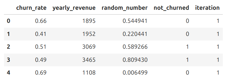
# Add a column with random numbers between 0 and 1 simulations['random_number'] = ( [random.uniform(0, 1) for _ in range(len(simulations))])
# Add a column 'not_churned' and set it to 1, then update it to 0 based on the random number simulations['not_churned'] = ( simulations['random_number'] >= simulations['churn_rate']).astype(int)
# Add an 'iteration' column starting from 1 to 10000 simulations['iteration'] = (simulations.index // 10) + 1
This gives a table like the one below:
head of simulations data frame / image by the author
We can summarize our results using the following code:
# Group by 'iteration' and calculate the required values
summary = simulations.groupby('iteration').agg(
    total_revenue=('yearly_revenue',
       lambda x: sum(x * simulations.loc[x.index, 'not_churned'])),
    total_churners=('not_churned', lambda x: 10 - sum(x))
).reset_index()
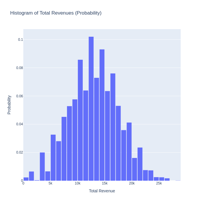
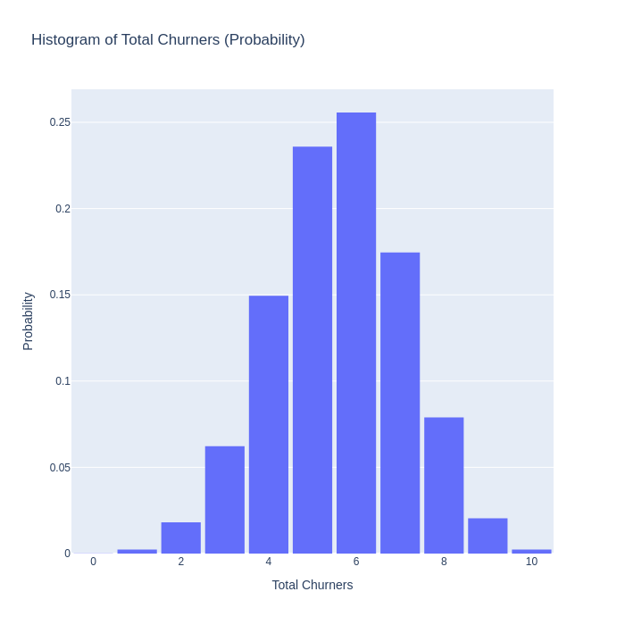
And finally, plotting this with plotly yields:
Histogram of total revenues / image by the authorHistogram of total churners / image by the author
The graphs above tell a much richer story than the two point estimates of 0.56 and 13034 we started with. We now understand much more about the possible outcomes we can expect to see, and we can have an informed discussion about what levels of churn and revenue we we find acceptable.
Continuing with the example above we could for example say that we would only be prepared to accept a 0.1 % chance of 8 or more churn events. Using individual customer price elasticities and simulation based forecasting, we could tweak the expected churn_rates for customers so that we could exactly achieve this outcome. This kind of customer base control is only achievable with an advanced CBM system.
The Importance of Competitor Pricing
One of the most important factors in pricing is the competitor price. How aggressive competitors are will to a large degree determine how flexible a company can be in its own pricing. This is especially true for commoditized businesses such as utilities or telcos where it’s hard for providers to differentiate. However, despite the importance of competitor pricing, many business choose not to integrate this data into their own price optimization algorithms.
The reasons for not including competitor pricing in price algorithms are varied. Some companies claim that it’s too difficult and time consuming to collect the data, and even if they started now, they still wouldn’t have all the history they need to train all the price elasticity models. Others say the prices of competitor products are not directly comparable to their own and that collecting them would be difficult. Finally, most companies also claim that they have price managers who manually monitor the market and when competitors make moves, they can adjust their own prices in response, so they don’t need to have this data in their algorithms.
The first argument can increasingly be mitigated by good web scraping and other intelligence gathering methods. If that is not enough, there are also sometimes agencies that can provide historic market data on prices for various industries and sectors. Regarding the second argument about not having comparable products, one can also use machine learning techniques to tease out the actual cost of individual product components. Another method is also to use different user personas that can be used to estimate the total monthly costs of a specific set of products or product.
Ultimately, not including competitor prices leaves the pricing algorithms and optimization engines at a disadvantage. In industries where price calculators and comparison websites make it increasingly easy for customers to get a grasp of the market, companies run a risk of being out-competed on price by more advanced competitors.
Conclusion
In this article we have discussed the main components of a customer base management system as well as some of the advanced features that contribute to making these systems invaluable. Personally, having built a few of these systems, I think the combination of price optimization algorithms — running on a broad dataset of internal and external data — coupled with a powerful visual interface in the form a dashboard is one of the most effective tools for managing customers. This combination of tools allows managers and executive leadership really take control of the customer management process and understand the strategic consequence of their actions.
As Jeff Bezos — one of the most customer-obsessed leaders — put it:
A commitment to customer management, underpinned by data and AI-driven insights, not only enhances customer satisfaction but also secures long-term value for stakeholders.
Thanks for reading!
Want to be notified whenever I publish a new article? ➡️ Subscribe to my newsletter here ⬅️. It’s free & you can unsubscribe at any time!
We use cookies on our website to give you the most relevant experience by remembering your preferences and repeat visits. By clicking “Accept”, you consent to the use of ALL the cookies.
This website uses cookies to improve your experience while you navigate through the website. Out of these, the cookies that are categorized as necessary are stored on your browser as they are essential for the working of basic functionalities of the website. We also use third-party cookies that help us analyze and understand how you use this website. These cookies will be stored in your browser only with your consent. You also have the option to opt-out of these cookies. But opting out of some of these cookies may affect your browsing experience.
Necessary cookies are absolutely essential for the website to function properly. These cookies ensure basic functionalities and security features of the website, anonymously.
Cookie
Duration
Description
cookielawinfo-checkbox-analytics
11 months
This cookie is set by GDPR Cookie Consent plugin. The cookie is used to store the user consent for the cookies in the category "Analytics".
cookielawinfo-checkbox-functional
11 months
The cookie is set by GDPR cookie consent to record the user consent for the cookies in the category "Functional".
cookielawinfo-checkbox-necessary
11 months
This cookie is set by GDPR Cookie Consent plugin. The cookies is used to store the user consent for the cookies in the category "Necessary".
cookielawinfo-checkbox-others
11 months
This cookie is set by GDPR Cookie Consent plugin. The cookie is used to store the user consent for the cookies in the category "Other.
cookielawinfo-checkbox-performance
11 months
This cookie is set by GDPR Cookie Consent plugin. The cookie is used to store the user consent for the cookies in the category "Performance".
viewed_cookie_policy
11 months
The cookie is set by the GDPR Cookie Consent plugin and is used to store whether or not user has consented to the use of cookies. It does not store any personal data.
Functional cookies help to perform certain functionalities like sharing the content of the website on social media platforms, collect feedbacks, and other third-party features.
Performance cookies are used to understand and analyze the key performance indexes of the website which helps in delivering a better user experience for the visitors.
Analytical cookies are used to understand how visitors interact with the website. These cookies help provide information on metrics the number of visitors, bounce rate, traffic source, etc.
Advertisement cookies are used to provide visitors with relevant ads and marketing campaigns. These cookies track visitors across websites and collect information to provide customized ads.