Don’t rush into the fancy title until you have read this.
Originally appeared here:
Are You Sure You Want to Become a Data Science Manager?
Go Here to Read this Fast! Are You Sure You Want to Become a Data Science Manager?

Don’t rush into the fancy title until you have read this.
Originally appeared here:
Are You Sure You Want to Become a Data Science Manager?
Go Here to Read this Fast! Are You Sure You Want to Become a Data Science Manager?
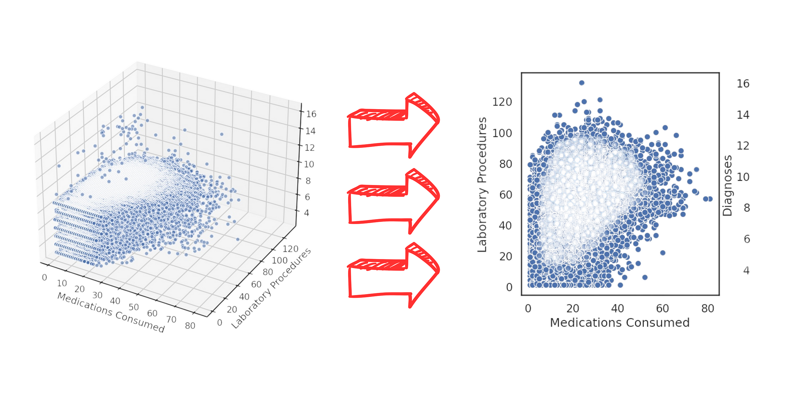

Mastering data visualization: from effective bar charts to common pitfalls like 3D visualizations.
Originally appeared here:
Data Visualization Techniques for Healthcare Data Analysis — Part III
Go Here to Read this Fast! Data Visualization Techniques for Healthcare Data Analysis — Part III
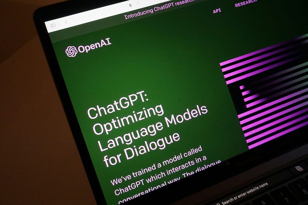
This November 30 marks the second anniversary of ChatGPT’s launch, an event that sent shockwaves through technology, society, and the economy. The space opened by this milestone has not always made it easy — or perhaps even possible — to separate reality from expectations. For example, this year Nvidia became the most valuable public company in the world during a stunning bullish rally. The company, which manufactures hardware used by models like ChatGPT, is now worth seven times what it was two years ago. The obvious question for everyone is: Is it really worth that much, or are we in the midst of collective delusion? This question — and not its eventual answer — defines the current moment.
AI is making waves not just in the stock market. Last month, for the first time in history, prominent figures in artificial intelligence were awarded the Nobel Prizes in Physics and Chemistry. John J. Hopfield and Geoffrey E. Hinton received the Physics Nobel for their foundational contributions to neural network development.
In Chemistry, Demis Hassabis, John Jumper, and David Baker were recognized for AlphaFold’s advances in protein design using artificial intelligence. These awards generated surprise on one hand and understandable disappointment among traditional scientists on the other, as computational methods took center stage.
In this context, I aim to review what has happened since that November, reflecting on the tangible and potential impact of generative AI to date, considering which promises have been fulfilled, which remain in the running, and which seem to have fallen by the wayside.
Let’s begin by recalling the day of the launch. ChatGPT 3.5 was a chatbot far superior to anything previously known in terms of discourse and intelligence capabilities. The difference between what was possible at the time and what ChatGPT could do generated enormous fascination and the product went viral rapidly: it reached 100 million users in just two months, far surpassing many applications considered viral (TikTok, Instagram, Pinterest, Spotify, etc.). It also entered mass media and public debate: AI landed in the mainstream, and suddenly everyone was talking about ChatGPT. To top it off, just a few months later, OpenAI launched GPT-4, a model vastly superior to 3.5 in intelligence and also capable of understanding images.
The situation sparked debates about the many possibilities and problems inherent to this specific technology, including copyright, misinformation, productivity, and labor market issues. It also raised concerns about the medium- and long-term risks of advancing AI research, such as existential risk (the “Terminator” scenario), the end of work, and the potential for artificial consciousness. In this broad and passionate discussion, we heard a wide range of opinions. Over time, I believe the debate began to mature and temper. It took us a while to adapt to this product because ChatGPT’s advancement left us all somewhat offside. What has happened since then?
As far as technology companies are concerned, these past two years have been a roller coaster. The appearance on the scene of OpenAI, with its futuristic advances and its CEO with a “startup” spirit and look, raised questions about Google’s technological leadership, which until then had been undisputed. Google, for its part, did everything it could to confirm these doubts, repeatedly humiliating itself in public. First came the embarrassment of Bard’s launch — the chatbot designed to compete with ChatGPT. In the demo video, the model made a factual error: when asked about the James Webb Space Telescope, it claimed it was the first telescope to photograph planets outside the solar system, which is false. This misstep caused Google’s stock to drop by 9% in the following week. Later, during the presentation of its new Gemini model — another competitor, this time to GPT-4 — Google lost credibility again when it was revealed that the incredible capabilities showcased in the demo (which could have placed it at the cutting edge of research) were, in reality, fabricated, based on much more limited capabilities.

Meanwhile, Microsoft — the archaic company of Bill Gates that produced the old Windows 95 and was as hated by young people as Google was loved — reappeared and allied with the small David, integrating ChatGPT into Bing and presenting itself as agile and defiant. “I want people to know we made them dance,” said Satya Nadella, Microsoft’s CEO, referring to Google. In 2023, Microsoft rejuvenated while Google aged.
This situation persisted, and OpenAI remained for some time the undisputed leader in both technical evaluations and subjective user feedback (known as “vibe checks”), with GPT-4 at the forefront. But over time, this changed and just as GPT-4 had achieved unique leadership by late 2022, by mid-2024 its close successor (GPT-4o) was competing with others of its caliber: Google’s Gemini 1.5 Pro, Anthropic’s Claude Sonnet 3.5, and xAI’s Grok 2. What innovation gives, innovation takes away.
This scenario could be shifting again with OpenAI’s recent announcement of o1 in September 2024 and rumors of new launches in December. For now, however, regardless of how good o1 may be (we’ll talk about it shortly), it doesn’t seem to have caused the same seismic impact as ChatGPT or conveyed the same sense of an unbridgeable gap with the rest of the competitive landscape.
To round out the scene of hits, falls, and epic comebacks, we must talk about the open-source world. This new AI era began with two gut punches to the open-source community. First, OpenAI, despite what its name implies, was a pioneer in halting the public disclosure of fundamental technological advancements. Before OpenAI, the norms of artificial intelligence research — at least during the golden era before 2022 — entailed detailed publication of research findings. During that period, major corporations fostered a positive feedback loop with academia and published papers, something previously uncommon. Indeed, ChatGPT and the generative AI revolution as a whole are based on a 2017 paper from Google, the famous Attention Is All You Need, which introduced the Transformer neural network architecture. This architecture underpins all current language models and is the “T” in GPT. In a dramatic plot twist, OpenAI leveraged this public discovery by Google to gain an advantage and began pursuing closed-door research, with GPT-4’s launch marking the turning point between these two eras: OpenAI disclosed nothing about the inner workings of this advanced model. From that moment, many closed models, such as Gemini 1.5 Pro and Claude Sonnet, began to emerge, fundamentally shifting the research ecosystem for the worse.
The second blow to the open-source community was the sheer scale of the new models. Until GPT-2, a modest GPU was sufficient to train deep learning models. Starting with GPT-3, infrastructure costs skyrocketed, and training models became inaccessible to individuals or most institutions. Fundamental advancements fell into the hands of a few major players.
But after these blows, and with everyone anticipating a knockout, the open-source world fought back and proved itself capable of rising to the occasion. For everyone’s benefit, it had an unexpected champion. Mark Zuckerberg, the most hated reptilian android on the planet, made a radical change of image by positioning himself as the flagbearer of open source and freedom in the generative AI field. Meta, the conglomerate that controls much of the digital communication fabric of the West according to its own design and will, took on the task of bringing open source into the LLM era with its LLaMa model line. It’s definitely a bad time to be a moral absolutist. The LLaMa line began with timid open licenses and limited capabilities (although the community made significant efforts to believe otherwise). However, with the recent releases of LLaMa 3.1 and 3.2, the gap with private models has begun to narrow significantly. This has allowed the open-source world and public research to remain at the forefront of technological innovation.
Over the past two years, research into ChatGPT-like models, known as large language models (LLMs), has been prolific. The first fundamental advancement, now taken for granted, is that companies managed to increase the context windows of models (how many words they can read as input and generate as output) while dramatically reducing costs per word. We’ve also seen models become multimodal, accepting not only text but also images, audio, and video as input. Additionally, they have been enabled to use tools — most notably, internet search — and have steadily improved in overall capacity.
On another front, various quantization and distillation techniques have emerged, enabling the compression of enormous models into smaller versions, even to the point of running language models on desktop computers (albeit sometimes at the cost of unacceptable performance reductions). This optimization trend appears to be on a positive trajectory, bringing us closer to small language models (SLMs) that could eventually run on smartphones.
On the downside, no significant progress has been made in controlling the infamous hallucinations — false yet plausible-sounding outputs generated by models. Once a quaint novelty, this issue now seems confirmed as a structural feature of the technology. For those of us who use this technology in our daily work, it’s frustrating to rely on a tool that behaves like an expert most of the time but commits gross errors or outright fabricates information roughly one out of every ten times. In this sense, Yann LeCun, the head of Meta AI and a major figure in AI, seems vindicated, as he had adopted a more deflationary stance on LLMs during the 2023 hype peak.
However, pointing out the limitations of LLMs doesn’t mean the debate is settled about what they’re capable of or where they might take us. For instance, Sam Altman believes the current research program still has much to offer before hitting a wall, and the market, as we’ll see shortly, seems to agree. Many of the advancements we’ve seen over the past two years support this optimism. OpenAI launched its voice assistant and an improved version capable of near-real-time interaction with interruptions — like human conversations rather than turn-taking. More recently, we’ve seen the first advanced attempts at LLMs gaining access to and control over users’ computers, as demonstrated in the GPT-4o demo (not yet released) and in Claude 3.5, which is available to end users. While these tools are still in their infancy, they offer a glimpse of what the near future could look like, with LLMs having greater agency. Similarly, there have been numerous breakthroughs in automating software engineering, highlighted by debatable milestones like Devin, the first “artificial software engineer.” While its demo was heavily criticized, this area — despite the hype — has shown undeniable, impactful progress. For example, in the SWE-bench benchmark, used to evaluate AI models’ abilities to solve software engineering problems, the best models at the start of the year could solve less than 13% of exercises. As of now, that figure exceeds 49%, justifying confidence in the current research program to enhance LLMs’ planning and complex task-solving capabilities.
Along the same lines, OpenAI’s recent announcement of the o1 model signals a new line of research with significant potential, despite the currently released version (o1-preview) not being far ahead from what’s already known. In fact, o1 is based on a novel idea: leveraging inference time — not training time — to improve the quality of generated responses. With this approach, the model doesn’t immediately produce the most probable next word but has the ability to “pause to think” before responding. One of the company’s researchers suggested that, eventually, these models could use hours or even days of computation before generating a response. Preliminary results have sparked high expectations, as using inference time to optimize quality was not previously considered viable. We now await subsequent models in this line (o2, o3, o4) to confirm whether it is as promising as it currently seems.
Beyond language models, these two years have seen enormous advancements in other areas. First, we must mention image generation. Text-to-image models began to gain traction even before chatbots and have continued developing at an accelerated pace, expanding into video generation. This field reached a high point with the introduction of OpenAI’s Sora, a model capable of producing extremely high-quality videos, though it was not released. Slightly less known but equally impressive are advances in music generation, with platforms like Suno and Udio, and in voice generation, which has undergone a revolution and achieved extraordinarily high-quality standards, led by Eleven Labs.
It has undoubtedly been two intense years of remarkable technological progress and almost daily innovations for those of us involved in the field.
If we turn our attention to the financial aspect of this phenomenon, we will see vast amounts of capital being poured into the world of AI in a sustained and growing manner. We are currently in the midst of an AI gold rush, and no one wants to be left out of a technology that its inventors, modestly, have presented as equivalent to the steam engine, the printing press, or the internet.
It may be telling that the company that has capitalized the most on this frenzy doesn’t sell AI but rather the hardware that serves as its infrastructure, aligning with the old adage that during a gold rush, a good way to get rich is by selling shovels and picks. As mentioned earlier, Nvidia has positioned itself as the most valuable company in the world, reaching a market capitalization of $3.5 trillion. For context, $3,500,000,000,000 is a figure far greater than France’s GDP.

On the other hand, if we look at the list of publicly traded companies with the highest market value, we see tech giants linked partially or entirely to AI promises dominating the podium. Apple, Nvidia, Microsoft, and Google are the top four as of the date of this writing, with a combined capitalization exceeding $12 trillion. For reference, in November 2022, the combined capitalization of these four companies was less than half of this value. Meanwhile, generative AI startups in Silicon Valley are raising record-breaking investments. The AI market is bullish.
While the technology advances fast, the business model for generative AI — beyond the major LLM providers and a few specific cases — remains unclear. As this bullish frenzy continues, some voices, including recent economics Nobel laureate Daron Acemoglu, have expressed skepticism about AI’s ability to justify the massive amounts of money being poured into it. For instance, in this Bloomberg interview, Acemoglu argues that current generative AI will only be able to automate less than 5% of existing tasks in the next decade, making it unlikely to spark the productivity revolution investors anticipate.
Is this AI fever or rather AI feverish delirium? For now, the bullish rally shows no signs of stopping, and like any bubble, it will be easy to recognize in hindsight. But while we’re in it, it’s unclear if there will be a correction and, if so, when it might happen. Are we in a bubble about to burst, as Acemoglu believes, or, as one investor suggested, is Nvidia on its way to becoming a $50 trillion company within a decade? This is the million-dollar question and, unfortunately, dear reader, I do not know the answer. Everything seems to indicate that, just like in the dot com bubble, we will emerge from this situation with some companies riding the wave and many underwater.
Let’s now discuss the broader social impact of generative AI’s arrival. The leap in quality represented by ChatGPT, compared to the socially known technological horizon before its launch, caused significant commotion, opening debates about the opportunities and risks of this specific technology, as well as the potential opportunities and risks of more advanced technological developments.
The problem of the future
The debate over the proximity of artificial general intelligence (AGI) — AI reaching human or superhuman capabilities — gained public relevance when Geoffrey Hinton (now a Physics Nobel laureate) resigned from his position at Google to warn about the risks such development could pose. Existential risk — the possibility that a super-capable AI could spiral out of control and either annihilate or subjugate humanity — moved out of the realm of fiction to become a concrete political issue. We saw prominent figures, with moderate and non-alarmist profiles, express concern in public debates and even in U.S. Senate hearings. They warned of the possibility of AGI arriving within the next ten years and the enormous problems this would entail.
The urgency that surrounded this debate now seems to have faded, and in hindsight, AGI appears further away than it did in 2023. It’s common to overestimate achievements immediately after they occur, just as it’s common to underestimate them over time. This latter phenomenon even has a name: the AI Effect, where major advancements in the field lose their initial luster over time and cease to be considered “true intelligence.” If today the ability to generate coherent discourse — like the ability to play chess — is no longer surprising, this should not distract us from the timeline of progress in this technology. In 1996, the Deep Blue model defeated chess champion Garry Kasparov. In 2016, AlphaGo defeated Go master Lee Sedol. And in 2022, ChatGPT produced high-quality, articulated speech, even challenging the famous Turing Test as a benchmark for determining machine intelligence. I believe it’s important to sustain discussions about future risks even when they no longer seem imminent or urgent. Otherwise, cycles of fear and calm prevent mature debate. Whether through the research direction opened by o1 or new pathways, it’s likely that within a few years, we’ll see another breakthrough on the scale of ChatGPT in 2022, and it would be wise to address the relevant discussions before that happens.
A separate chapter on AGI and AI safety involves the corporate drama at OpenAI, worthy of prime-time television. In late 2023, Sam Altman was abruptly removed by the board of directors. Although the full details were never clarified, Altman’s detractors pointed to an alleged culture of secrecy and disagreements over safety issues in AI development. The decision sparked an immediate rebellion among OpenAI employees and drew the attention of Microsoft, the company’s largest investor. In a dramatic twist, Altman was reinstated, and the board members who removed him were dismissed. This conflict left a rift within OpenAI: Jan Leike, the head of AI safety research, joined Anthropic, while Ilya Sutskever, OpenAI’s co-founder and a central figure in its AI development, departed to create Safe Superintelligence Inc. This seems to confirm that the original dispute centered around the importance placed on safety. To conclude, recent rumors suggest OpenAI may lose its nonprofit status and grant shares to Altman, triggering another wave of resignations within the company’s leadership and intensifying a sense of instability.
From a technical perspective, we saw a significant breakthrough in AI safety from Anthropic. The company achieved a fundamental milestone in LLM interpretability, helping to better understand the “black box” nature of these models. Through their discovery of the polysemantic nature of neurons and a method for extracting neural activation patterns representing concepts, the primary barrier to controlling Transformer models seems to have been broken — at least in terms of their potential to deceive us. The ability to deliberately alter circuits actively modifying the observable behavior in these models is also promising and brought some peace of mind regarding the gap between the capabilities of the models and our understanding of them.
The problems of the present
Setting aside the future of AI and its potential impacts, let’s focus on the tangible effects of generative AI. Unlike the arrival of the internet or social media, this time society seemed to react quickly, demonstrating concern about the implications and challenges posed by this new technology. Beyond the deep debate on existential risks mentioned earlier — centered on future technological development and the pace of progress — the impacts of existing language models have also been widely discussed. The main issues with generative AI include the fear of amplifying misinformation and digital pollution, significant problems with copyright and private data use, and the impact on productivity and the labor market.
Regarding misinformation, this study suggests that, at least for now, there hasn’t been a significant increase in exposure to misinformation due to generative AI. While this is difficult to confirm definitively, my personal impressions align: although misinformation remains prevalent — and may have even increased in recent years — it hasn’t undergone a significant phase change attributable to the emergence of generative AI. This doesn’t mean misinformation isn’t a critical issue today. The weaker thesis here is that generative AI doesn’t seem to have significantly worsened the problem — at least not yet.
However, we have seen instances of deep fakes, such as recent cases involving AI-generated pornographic material using real people’s faces, and more seriously, cases in schools where minors — particularly young girls — were affected. These cases are extremely serious, and it’s crucial to bolster judicial and law enforcement systems to address them. However, they appear, at least preliminarily, to be manageable and, in the grand scheme, represent relatively minor impacts compared to the speculative nightmare of misinformation fueled by generative AI. Perhaps legal systems will take longer than we would like, but there are signs that institutions may be up to the task at least as far as deep fakes of underage porn are concerned, as illustrated by the exemplary 18-year sentence received by a person in the United Kingdom for creating and distributing this material.
Secondly, concerning the impact on the labor market and productivity — the flip side of the market boom — the debate remains unresolved. It’s unclear how far this technology will go in increasing worker productivity or in reducing or increasing jobs. Online, one can find a wide range of opinions about this technology’s impact. Claims like “AI replaces tasks, not people” or “AI won’t replace you, but a person using AI will” are made with great confidence yet without any supporting evidence — something that ironically recalls the hallucinations of a language model. It’s true that ChatGPT cannot perform complex tasks, and those of us who use it daily know its significant and frustrating limitations. But it’s also true that tasks like drafting professional emails or reviewing large amounts of text for specific information have become much faster. In my experience, productivity in programming and data science has increased significantly with AI-assisted programming environments like Copilot or Cursor. In my team, junior profiles have gained greater autonomy, and everyone produces code faster than before. That said, the speed in code production could be a double-edged sword, as some studies suggest that code generated with generative AI assistants may be of lower quality than code written by humans without such assistance.
If the impact of current LLMs isn’t entirely clear, this uncertainty is compounded by significant advancements in associated technologies, such as the research line opened by o1 or the desktop control anticipated by Claude 3.5. These developments increase the uncertainty about the capabilities these technologies could achieve in the short term. And while the market is betting heavily on a productivity boom driven by generative AI, many serious voices downplay the potential impact of this technology on the labor market, as noted earlier in the discussion of the financial aspect of the phenomenon. In principle, the most significant limitations of this technology (e.g., hallucinations) have not only remained unresolved but now seem increasingly unlikely to be resolved. Meanwhile, human institutions have proven less agile and revolutionary than the technology itself, cooling the conversation and dampening the enthusiasm of those envisioning a massive and immediate impact.
In any case, the promise of a massive revolution in the workplace, if it is to materialize, has not yet materialized in at least these two years. Considering the accelerated adoption of this technology (according to this study, more than 24% of American workers today use generative AI at least once a week) and assuming that the first to adopt it are perhaps those who find the greatest benefits, we can think that we have already seen enough of the productivity impact of this technology. In terms of my professional day-to-day and that of my team, the productivity impacts so far, while noticeable, significant, and visible, have also been modest.
Another major challenge accompanying the rise of generative AI involves copyright issues. Content creators — including artists, writers, and media companies — have expressed dissatisfaction over their works being used without authorization to train AI models, which they consider a violation of their intellectual property rights. On the flip side, AI companies often argue that using protected material to train models is covered under “fair use” and that the production of these models constitutes legitimate and creative transformation rather than reproduction.
This conflict has resulted in numerous lawsuits, such as Getty Images suing Stability AI for the unauthorized use of images to train models, or lawsuits by artists and authors, like Sarah Silverman, against OpenAI, Meta, and other AI companies. Another notable case involves record companies suing Suno and Udio, alleging copyright infringement for using protected songs to train generative music models.
In this futuristic reinterpretation of the age-old divide between inspiration and plagiarism, courts have yet to decisively tip the scales one way or the other. While some aspects of these lawsuits have been allowed to proceed, others have been dismissed, maintaining an atmosphere of uncertainty. Recent legal filings and corporate strategies — such as Adobe, Google, and OpenAI indemnifying their clients — demonstrate that the issue remains unresolved, and for now, legal disputes continue without a definitive conclusion.

The regulatory framework for AI has also seen significant progress, with the most notable development on this side of the globe being the European Union’s approval of the AI Act in March 2024. This legislation positioned Europe as the first bloc in the world to adopt a comprehensive regulatory framework for AI, establishing a phased implementation system to ensure compliance, set to begin in February 2025 and proceed gradually.
The AI Act classifies AI risks, prohibiting cases of “unacceptable risk,” such as the use of technology for deception or social scoring. While some provisions were softened during discussions to ensure basic rules applicable to all models and stricter regulations for applications in sensitive contexts, the industry has voiced concerns about the burden this framework represents. Although the AI Act wasn’t a direct consequence of ChatGPT and had been under discussion beforehand, its approval was accelerated by the sudden emergence and impact of generative AI models.
With these tensions, opportunities, and challenges, it’s clear that the impact of generative AI marks the beginning of a new phase of profound transformations across social, economic, and legal spheres, the full extent of which we are only beginning to understand.
I approached this article thinking that the ChatGPT boom had passed and its ripple effects were now subsiding, calming. Reviewing the events of the past two years convinced me otherwise: they’ve been two years of great progress and great speed.
These are times of excitement and expectation — a true springtime for AI — with impressive breakthroughs continuing to emerge and promising research lines waiting to be explored. On the other hand, these are also times of uncertainty. The suspicion of being in a bubble and the expectation of a significant emotional and market correction are more than reasonable. But as with any market correction, the key isn’t predicting if it will happen but knowing exactly when.
What will happen in 2025? Will Nvidia’s stock collapse, or will the company continue its bullish rally, fulfilling the promise of becoming a $50 trillion company within a decade? And what will happen to the AI stock market in general? And what will become of the reasoning model research line initiated by o1? Will it hit a ceiling or start showing progress, just as the GPT line advanced through versions 1, 2, 3, and 4? How much will today’s rudimentary LLM-based agents that control desktops and digital environments improve overall?
We’ll find out sooner rather than later, because that’s where we’re headed.

ChatGPT: Two Years Later was originally published in Towards Data Science on Medium, where people are continuing the conversation by highlighting and responding to this story.
Originally appeared here:
ChatGPT: Two Years Later

TL;DR — We achieve the same functionality as LangChains’ Parent Document Retriever (link) by utilizing metadata queries. You can explore the code here.
Retrieval-augmented generation (RAG) is currently one of the hottest topics in the world of LLM and AI applications.
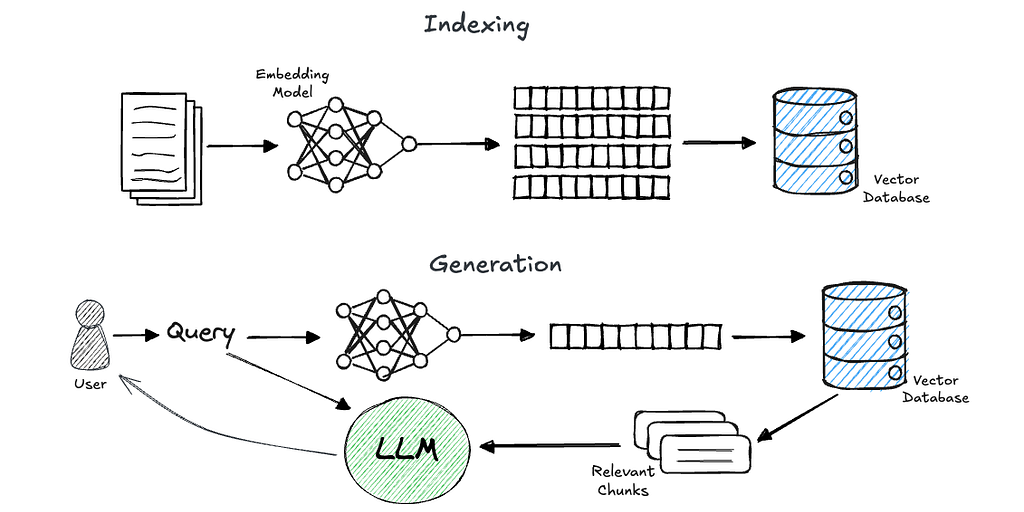
In short, RAG is a technique for grounding a generative models’ response on chosen knowledge sources. It comprises two phases: retrieval and generation.
A commonly used approach to achieve efficient and accurate retrieval is through the usage of embeddings. In this approach, we preprocess users’ data (let’s assume plain text for simplicity) by splitting the documents into chunks (such as pages, paragraphs, or sentences). We then use an embedding model to create a meaningful, numerical representation of these chunks, and store them in a vector database. Now, when a query comes in, we embed it as well and perform a similarity search using the vector database to retrieve the relevant information
If you are completely new to this concept, I’d recommend deeplearning.ai great course, LangChain: Chat with Your Data.
“Parent Document Retrieval” or “Sentence Window Retrieval” as referred by others, is a common approach to enhance the performance of retrieval methods in RAG by providing the LLM with a broader context to consider.
In essence, we divide the original documents into relatively small chunks, embed each one, and store them in a vector database. Using such small chunks (a sentence or a couple of sentences) helps the embedding models to better reflect their meaning [1].
Then, at retrieval time, we do not return the most similar chunk as found by the vector database only, but also its surrounding context (chunks) in the original document. That way, the LLM will have a broader context, which, in many cases, helps generate better answers.
LangChain supports this concept via Parent Document Retriever [2]. The Parent Document Retriever allows you to: (1) retrieve the full document a specific chunk originated from, or (2) pre-define a larger “parent” chunk, for each smaller chunk associated with that parent.
Let’s explore the example from LangChains’ docs:
# This text splitter is used to create the parent documents
parent_splitter = RecursiveCharacterTextSplitter(chunk_size=2000)
# This text splitter is used to create the child documents
# It should create documents smaller than the parent
child_splitter = RecursiveCharacterTextSplitter(chunk_size=400)
# The vectorstore to use to index the child chunks
vectorstore = Chroma(
    collection_name="split_parents", embedding_function=OpenAIEmbeddings()
)
# The storage layer for the parent documents
store = InMemoryStore()
retriever = ParentDocumentRetriever(
    vectorstore=vectorstore,
    docstore=store,
    child_splitter=child_splitter,
    parent_splitter=parent_splitter,
)
retrieved_docs = retriever.invoke("justice breyer")
In my opinion, there are two disadvantages of the LangChains’ approach:
Indeed, a few questions have been raised regarding this issue [3].
Here I’ll also mention that Llama-index has its own SentenceWindowNodeParser [4], which generally has the same disadvantages.
In what follows, I’ll present another approach to achieve this useful feature that addresses the two disadvantages mentioned above. In this approach, we’ll be only using the vector store that is already in use.
To be precise, we’ll be using a vector store that supports the option to perform metadata queries only, without any similarity search involved. Here, I’ll present an implementation for ChromaDB and Milvus. This concept can be easily adapted to any vector database with such capabilities. I’ll refer to Pinecone for example in the end of this tutorial.
The general concept
The concept is straightforward:
For example, assuming you’ve indexed a document named example.pdf in 80 chunks. Then, for some query, you find that the closest vector is the one with the following metadata:
{document_id: "example.pdf", sequence_number: 20}
You can easily get all vectors from the same document with sequence numbers from 15 to 25.
Let’s see the code.
Here, I’m using:
chromadb==0.4.24
langchain==0.2.8
pymilvus==2.4.4
langchain-community==0.2.7
langchain-milvus==0.1.2
The only interesting thing to notice below is the metadata associated with each chunk, which will allow us to perform the search.
from langchain_community.document_loaders import PyPDFLoader
from langchain_core.documents import Document
from langchain_text_splitters import RecursiveCharacterTextSplitter

document_id = "example.pdf"

def preprocess_file(file_path: str) -> list[Document]:
    """Load pdf file, chunk and build appropriate metadata"""
    loader = PyPDFLoader(file_path=file_path)
    pdf_docs = loader.load()

    text_splitter = RecursiveCharacterTextSplitter(
        chunk_size=1000,
        chunk_overlap=0,
    )

    docs = text_splitter.split_documents(documents=pdf_docs)
    chunks_metadata = [
        {"document_id": file_path, "sequence_number": i} for i, _ in enumerate(docs)
    ]
    for chunk, metadata in zip(docs, chunks_metadata):
        chunk.metadata = metadata

    return docs
Now, lets implement the actual retrieval in Milvus and Chroma. Note that I’ll use the LangChains’ objects and not the native clients. I do this because I assume developers might want to keep LangChains’ useful abstraction. On the other hand, it will require us to perform some minor hacks to bypass these abstractions in a database-specific way, so you should take that into consideration. Anyway, the concept remains the same.
Again, let’s assume for simplicity we want only the most similar vector (“top 1”). Next, we’ll extract the associated document_id and its sequence number. This will allow us to retrieve the surrounding window.
from langchain_community.vectorstores import Milvus, Chroma
from langchain_community.embeddings import DeterministicFakeEmbedding

embedding = DeterministicFakeEmbedding(size=384) # Just for the demo :)

def parent_document_retrieval(
    query: str, client: Milvus | Chroma, window_size: int = 4
):
    top_1 = client.similarity_search(query=query, k=1)[0]
    doc_id = top_1.metadata["document_id"]
    seq_num = top_1.metadata["sequence_number"]
    ids_window = [seq_num + i for i in range(-window_size, window_size, 1)]
    # ...
Now, for the window/parent retrieval, we’ll dig under the Langchain abstraction, in a database-specific way.
For Milvus:
  if isinstance(client, Milvus):
        expr = f"document_id LIKE '{doc_id}' && sequence_number in {ids_window}"
        res = client.col.query(
            expr=expr, output_fields=["sequence_number", "text"], limit=len(ids_window)
        )  # This is Milvus specific
        docs_to_return = [
            Document(
                page_content=d["text"],
                metadata={
                    "sequence_number": d["sequence_number"],
                    "document_id": doc_id,
                },
            )
            for d in res
        ]
    # ...
For Chroma:
    elif isinstance(client, Chroma):
        expr = {
            "$and": [
                {"document_id": {"$eq": doc_id}},
                {"sequence_number": {"$gte": ids_window[0]}},
                {"sequence_number": {"$lte": ids_window[-1]}},
            ]
        }
        res = client.get(where=expr)  # This is Chroma specific
        texts, metadatas = res["documents"], res["metadatas"]
        docs_to_return = [
            Document(
                page_content=t,
                metadata={
                    "sequence_number": m["sequence_number"],
                    "document_id": doc_id,
                },
            )
            for t, m in zip(texts, metadatas)
        ]
and don’t forget to sort it by the sequence number:
    docs_to_return.sort(key=lambda x: x.metadata["sequence_number"])
    return docs_to_return
For your convenience, you can explore the full code here.
As far as I know, there’s no native way to perform such a metadata query in Pinecone, but you can natively fetch vectors by their ID (https://docs.pinecone.io/guides/data/fetch-data).
Hence, we can do the following: each chunk will get a unique ID, which is essentially a concatenation of the document_id and the sequence number. Then, given a vector retrieved in the similarity search, you can dynamically create a list of the IDs of the surrounding chunks and achieve the same result.
It’s worth mentioning that vector databases were not designed to perform “regular” database operations and usually not optimized for that, and each database will perform differently. Milvus, for example, will support building indices over scalar fields (“metadata”) which can optimize these kinds of queries.
Also, note that it requires additional query to the vector database. First we retrieved the most similar vector, and then we performed additional query to get the surrounding chunks in the original document.
And of course, as seen from the code examples above, the implementation is vector database-specific and is not supported natively by the LangChains’ abstraction.
In this blog we introduced an implementation to achieve sentence-window retrieval, which is a useful retrieval technique used in many RAG applications. In this implementation we’ve used only the vector database which is already in use anyway, and also support the option to modify dynamically the the size of the surrounding window retrieved.
[1] ARAGOG: Advanced RAG Output Grading, https://arxiv.org/pdf/2404.01037, section 4.2.2
[2] https://python.langchain.com/v0.1/docs/modules/data_connection/retrievers/parent_document_retriever/
[3] Some related issues:
– https://github.com/langchain-ai/langchain/issues/14267
– https://github.com/langchain-ai/langchain/issues/20315
– https://stackoverflow.com/questions/77385587/persist-parentdocumentretriever-of-langchain
[4] https://docs.llamaindex.ai/en/stable/api_reference/node_parsers/sentence_window/
LangChain’s Parent Document Retriever — Revisited was originally published in Towards Data Science on Medium, where people are continuing the conversation by highlighting and responding to this story.
Originally appeared here:
LangChain’s Parent Document Retriever — Revisited
Go Here to Read this Fast! LangChain’s Parent Document Retriever — Revisited


What do a network of financial transactions and a protein structure have in common? They’re both poorly modeled in Euclidean (x, y) space and require encoding complex, large, and heterogeneous graphs to truly grok.
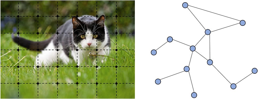
Graphs are the natural way to represent relational data in financial networks and protein structures. They capture the relationships and interactions between entities, such as transactions between accounts in financial systems or bonds and spatial proximities between amino acids in proteins. However, more widely known deep learning architectures like RNNs/CNNs and Transformers fail to model graphs effectively.
You might ask yourself why we can’t just map these graphs into 3D space? If we were to force them into a 3D grid:
Given these limitations, Graph Neural Networks (GNNs) serve as a powerful alternative. In this continuation of our series on Machine Learning for Biology applications, we’ll explore how GNNs can address these challenges.
As always, we’ll start with the more familiar topic of fraud detection and then learn how similar concepts are applied in biology.
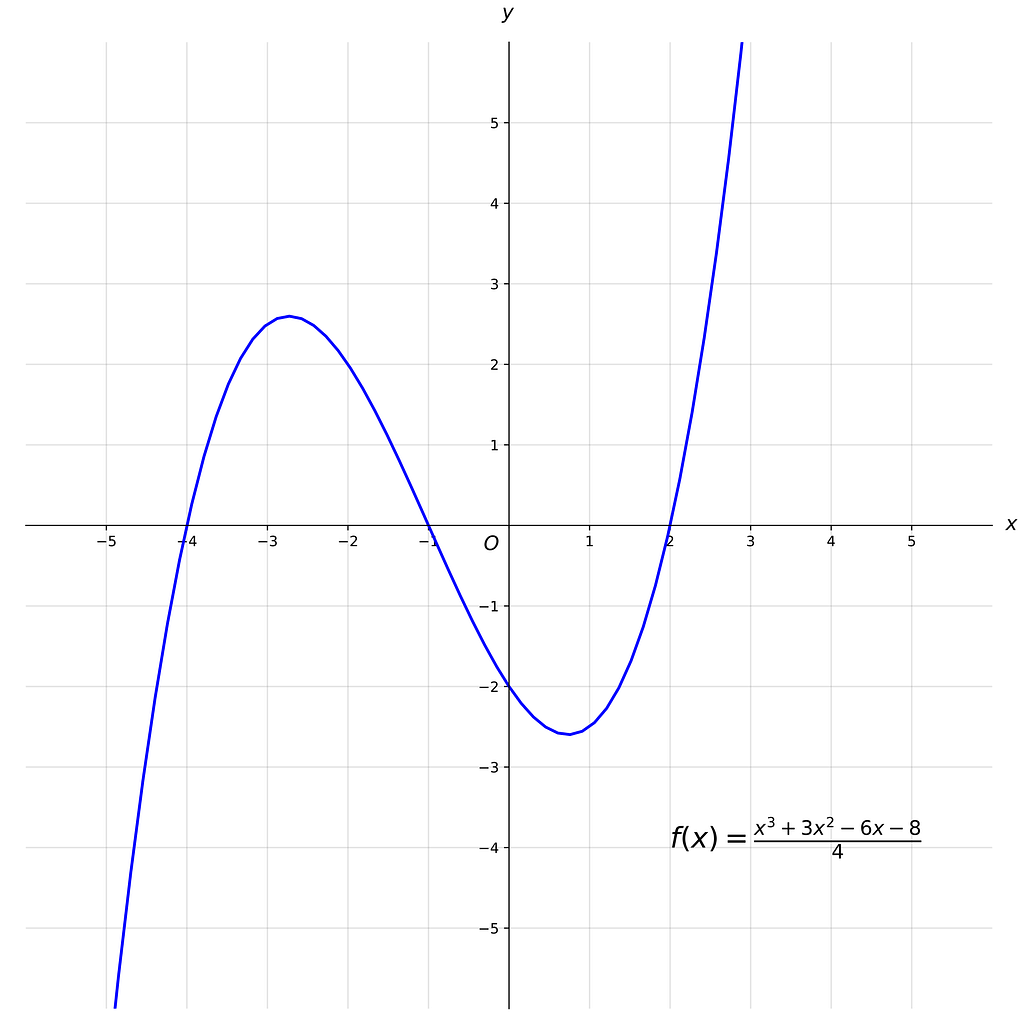
To be crystal clear, let’s first define what a graph is. We remember plotting graphs on x, y axes in grade school but what we were really doing there was graphing a function where we plotted the points of f(x)=y. We when talk about a “graph” in the context of GNNs, we mean to model pairwise relations between objects where each object is a node and the relationships are edges.
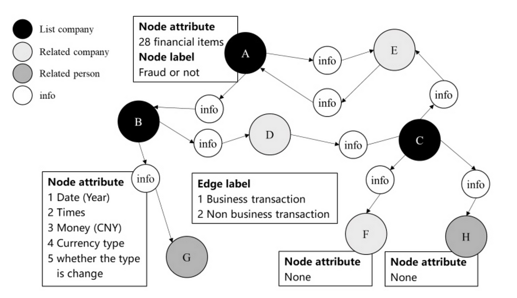
In a financial network, the nodes are accounts and the edges are the transactions. The graph would be constructed from related party transactions (RPT) and could be enriched with attributes (e.g. time, amount, currency).

Traditional rules-based and machine-learning methods often operate on a single transaction or entity. This limitation fails to account for how transactions are connected to the wider network. Because fraudsters often operate across multiple transactions or entities, fraud can go undetected.
By analyzing a graph, we can capture dependencies and patterns between direct neighbors and more distant connections. This is crucial for detecting laundering where funds are moved through multiple transactions to obscure their origin. GNNs illuminate the dense subgraphs created by laundering methods.
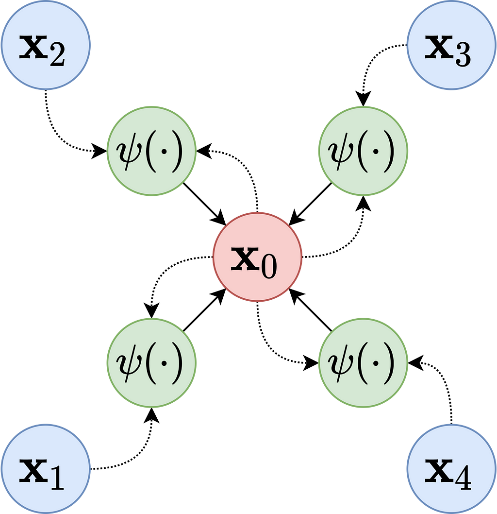
Like other deep learning methods, the goal is to create a representation or embedding from the dataset. In GNNs, these node embeddings are created using a message-passing framework. Messages pass between nodes iteratively, enabling the model to learn both the local and global structure of the graph. Each node embedding is updated based on the aggregation of its neighbors’ features.
A generalization of the framework works as follows:
After the node embeddings are learned, a fraud score can be calculated in a few different ways:
Now that we have a foundational understanding of GNNs for a familiar problem, we can turn to another application of GNNs: predicting the functions of proteins.
We’ve seen huge advances in protein folding prediction via AlphaFold 2 and 3 and protein design via RFDiffusion. However, protein function prediction remains challenging. Function prediction is vital for many reasons but is particularly important in biosecurity to predict if DNA will be parthenogenic before sequencing. Tradional methods like BLAST rely on sequence similarity searching and do not incoperate any structural data.
Today, GNNs are beginning to make meaningful progress in this area by leveraging graph representations of proteins to model relationships between residues and their interactions. There are considered to be well-suited for protein function prediction as well as, identifying binding sites for small molecules or other proteins and classifying enzyme families based on active site geometry.
In many examples:
The rational behind this approach is a graph’s inherent ability to capture long-range interactions between residues that are distant in the sequence but close in the folded structure. This is similar to why transformer archicture was so helpful for AlphaFold 2, which allowed for parallelized computation across all pairs in a sequence.
To make the graph information-dense, each node can be enriched with features like residue type, chemical properties, or evolutionary conservation scores. Edges can optionally be enriched with attributes like the type of chemical bonds, proximity in 3D space, and electrostatic or hydrophobic interactions.
DeepFRI is a GNN approach for predicting protein functions from structure (specifically a Graph Convolutional Network (GCN)). A GCN is a specific type of GNN that extends the idea of convolution (used in CNNs) to graph data.
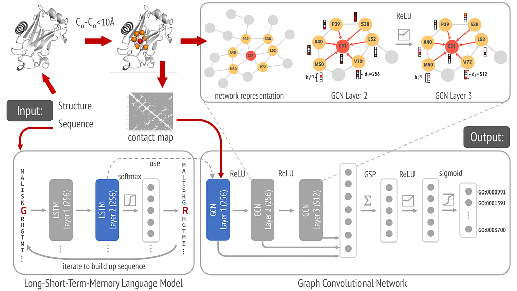
In DeepFRI, each amino acid residue is a node enriched by attributes such as:
Each edge is defined to capture spatial relationships between amino acid residues in the protein structure. An edge exists between two nodes (residues) if their distance is below a certain threshold, typically 10 Å. In this application, there are no attributes to the edges, which serve as unweighted connections.
The graph is initialized with node features LSTM-generated sequence embeddings along with the residue-specific features and edge information created from a residue contact map.
Once the graph is defined, message passing occurs through adjacency-based convolutions at each of the three layers. Node features are aggregated from neighbors using the graph’s adjacency matrix. Stacking multiple GCN layers allows embeddings to capture information from increasingly larger neighborhoods, starting with direct neighbors and extending to neighbors of neighbors etc.
The final node embeddings are globally pooled to create a protein-level embedding, which is then used to classify proteins into hierarchically related functional classes (GO terms). Classification is performed by passing the protein-level embeddings through fully connected layers (dense layers) with sigmoid activation functions, optimized using a binary cross-entropy loss function. The classification model is trained on data derived from protein structures (e.g., from the Protein Data Bank) and functional annotations from databases like UniProt or Gene Ontology.
Cheers and if you liked this post, check out my other articles on Machine Learning and Biology.
Graph Neural Networks: Fraud Detection and Protein Function Prediction was originally published in Towards Data Science on Medium, where people are continuing the conversation by highlighting and responding to this story.
Originally appeared here:
Graph Neural Networks: Fraud Detection and Protein Function Prediction
Go Here to Read this Fast! Graph Neural Networks: Fraud Detection and Protein Function Prediction
Learn how to implement coding best practices to avoid tech debts
Originally appeared here:
Leverage Python Inheritance in ML projects
Go Here to Read this Fast! Leverage Python Inheritance in ML projects

In many real-world machine learning tasks, the population being studied is often diverse and heterogeneous. This variability presents unique challenges, particularly in regression and classification tasks where a single, generalized model may fail to capture important nuances within the data. For example, segmenting customers in marketing campaigns, estimating the sales of a new product using data from comparable products, or diagnosing a patient with limited medical history based on similar cases all highlight the need for models that can adapt to different subpopulations.
This concept of segmentation is not new. Models like k-Nearest Neighbors or Decision Trees already implicitly leverage the idea of dividing the input space into regions that share somewhat similar properties. However, these approaches are often heuristic and do not explicitly optimize for both clustering and prediction simultaneously.
In this article, we approach this challenge from an optimization perspective, following the literature on Predictive and Prescriptive Analytics ([8]). Specifically, we focus on the task of joint clustering and prediction, which seeks to segment the data into clusters while simultaneously fitting a predictive model within each cluster. This approach has gained attention for its ability to bridge the gap between data-driven decision-making and actionable insights and extracting more information from data than other traditional methods (see [2] for instance).
After presenting some theoretical insights on Clustering and Regression from recent literature, we introduce a novel Classification method (Cluster While Classify) and show its superior performance in low data environments.
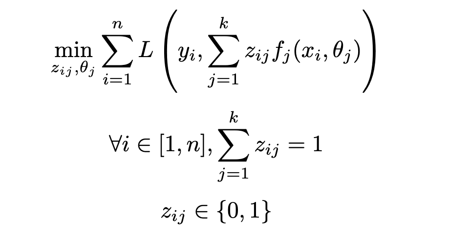
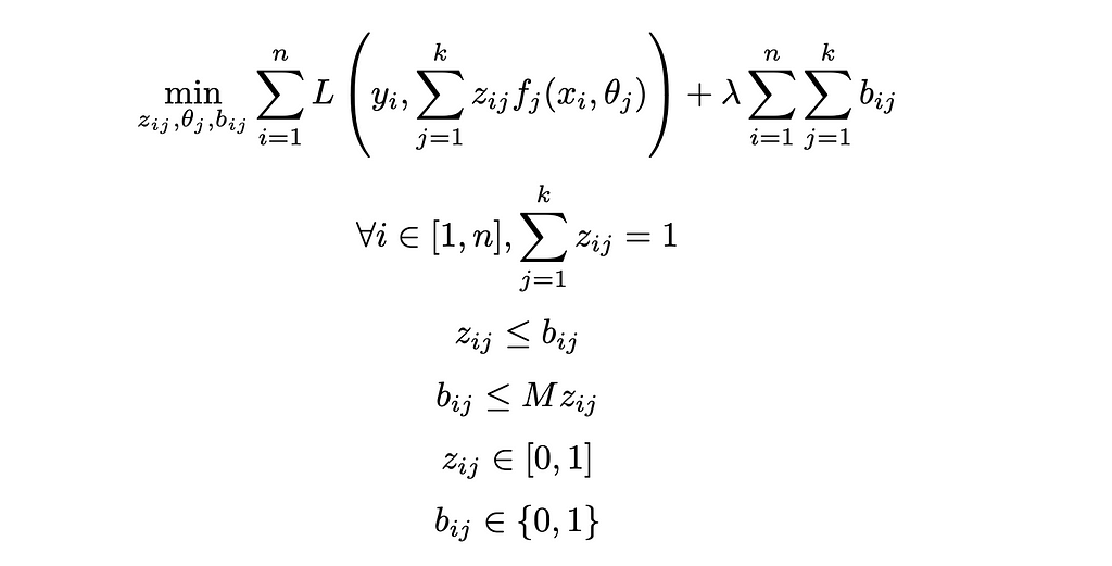
We first start with formulating the problem of optimal clustering and regression — jointly — to achieve the best fitting and prediction performance. Some formal notations and assumptions:
As ultimately a regression problem, the goal of the task is to find the set of parameters (i.e. parameters for each regression model θⱼ as well as the additional cluster assignment variables zᵢⱼ) minimizing the loss function L:
One of the most natural approaches — and used in numerous practical application of clustering and regression analyses — is the naive Cluster Then Regress (CTR) approach — i.e. first running clustering then run a regression model on the static result of this clustering. It is known to be suboptimal: namely, error propagates from the clustering step to the regression step, and erroneous assignments can have significant consequences on the performance.
We will mathematically show this suboptimality. When running a CTR approach, we first assign the clusters, and then fit the k regression models with cluster assignments as static. This translates to the following nested optimization:
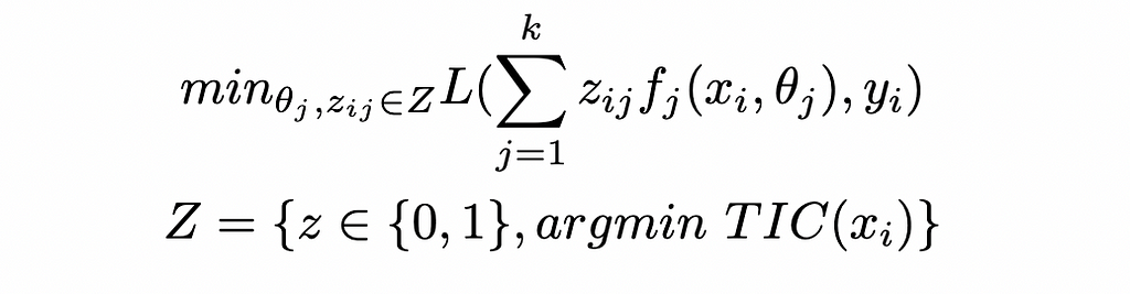
With TIC a measure of Total Intra Cluster Variance. Given that Z is included in ({0, 1})ⁿ, we see that the CTR approach solves a problem that is actually more constrained the the original one (i.e. further constraining the (zᵢⱼ) to be in Z rather than free in ({0, 1})ⁿ). Consequently, this yields a suboptimal result for the original optimization.
Unfortunately, attempting to directly solve the original optimization presented in section 1.1 can be intractable in practice, (Mixed integer optimization problem, with potential non-linearity coming from the choice of regression models). [1] presents a fast and easy — but approximate — solution to jointly learn the optimal cluster assignment and regression models: doing it iteratively. In practice, the Cluster While Regress (CWR) is:
Besides the iterative nature of this method, it presents a key difference with the CTR approach: clustering and regression optimize for the same objective function.
Applying the previous reasoning to classification, we have 2 different routes:
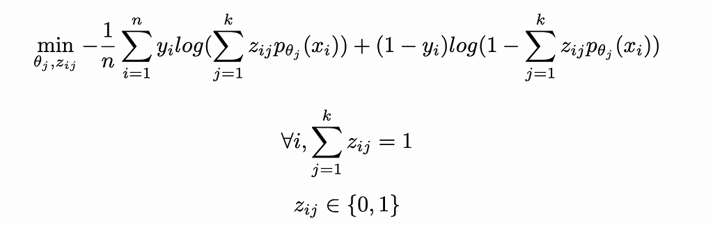
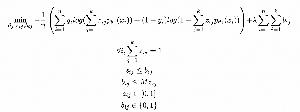
A few modifications are to be done to the objective problem, namely the loss function L which becomes a classification loss. For simplicity, we will focus on binary classification, but this formulation can easily be extended.
A popular loss function when doing binary classification is the binary cross-entropy loss:

Where p is the prediction of the classification model parametrized by θ in terms of probability of being in the class 1.
Introducing the clustering into this loss yields the following optimization model:
Similarly to CWR, we can find an approximate solution to this problem through the same algorithm, i.e. iteratively fitting the clustering and classification steps until convergence.
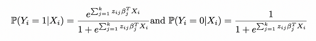
In this specific case, the probabilities are of the form:

Injecting this formula in the objective function of the optimization problem gives:

Inference with both CWR and CWC models can be done with the following process, described in details in [1]:
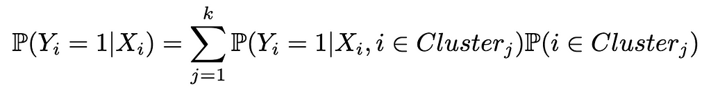
Where P(Yᵢ = 1| Xᵢ, i ∈ Clusterⱼ) is given by j-th classification model fitted and P(i ∈ Clusterⱼ) comes from the cluster assignment classifier.
Generalization to non-integer weights relaxes the integer constraint on the z variables. This corresponds to the case of an algorithm allowing for (probabilistic) assignment to multiple clusters, e.g. Soft K-Means — in this case assignments become weights between 0 and 1.
The fitting and inference processes are very similar to previously, with the sole differences being during the fitting phase: calibrating the regression / classification models on each cluster is replaced with calibrated the weighted regressions (e.g. Weighted Least Squares) or weighted classifications (e.g. Weighted Logistic Regression — see [4] for an example), with weight matrices Wⱼ = Diag(zᵢⱼ) with i corresponding to all the indices such that zᵢⱼ > 0. Note that unlike methods such as Weighted Least Squares, weights here are given when fitting the regression.
This generalization has 2 direct implications on the problem at hand:
[1] already included a regularization term for the regression coefficients, which corresponds to having regularized fⱼ models: in the case of a Linear Regression, this would means for instance that fⱼ is a LASSO or a Ridge rather than a simple OLS.
Yet, the proposal here is different, as we suggest additional regularization, this time penalizing the non-zero zᵢⱼ: the rationale is that we want to limit the number of models implicated in the fitting / inference of a given data point to reduce noise and degrees of freedom to prevent overfitting.
In practice, we add a new set of binary variables (bᵢⱼ) equal to 1 if zᵢⱼ > 0 and 0 otherwise. We can write it as linear constraints using the big M method:

All in, we have the two optimization models:
Generalized Cluster While Regress:
Generalized Cluster While Classify:
These problems can be efficiently solved with First Order methods or Cutting Planes — see [3] for details.
We evaluate these methods on 3 different benchmark datasets to illustrate 3 key aspects of their behavior and performance:
Some implementation details:
The Diabetes 130-US Hospitals dataset (1999–2008) ([5]) contains information about diabetes patients admitted to 130 hospitals across the United States over a 9-year period. The goal of the classification task is to predict whether a given diabetes patient will be readmitted. We will simplify the classes into 2 classes — readmitted or not — instead of 3 (readmitted after less than 30 days, readmitted after more than 30 days, not readmitted). We will also consider a subset of 20,000 data points instead of the full 100,000 instances for faster training.
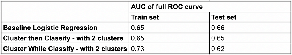
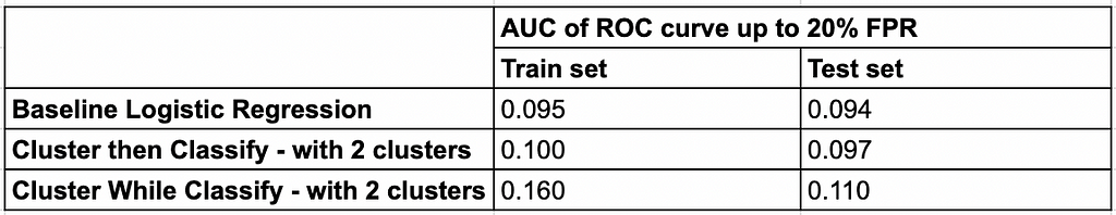
The MAGIC Gamma Telescope dataset ([6]) contains data from an observatory aimed at classifying high-energy cosmic ray events as either gamma rays (signal) or hadrons (background). A specificity of this dataset is the non-symmetric nature of errors: given the higher cost of false positives (misclassifying hadrons as gamma rays), accuracy is not suitable. Instead, performance is evaluated using the ROC curve and AUC, with a focus on maintaining a false positive rate (FPR) below 20% — as explained in [6].
The Parkinson’s dataset ([7]) contains data collected from voice recordings of 195 individuals, including both those with Parkinson’s disease and healthy controls. The dataset is used for classifying the presence or absence of Parkinson’s based on features extracted from speech signals. A key challenge of this dataset is the low number of datapoints, which makes generalization with traditional ML methods difficult. We can diagnose this generalization challenge and overfitting by comparing the performance numbers on train vs test sets.
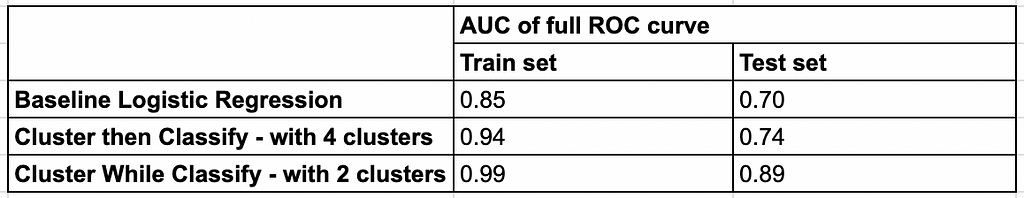
The study of baseline and joint clustering and classification approaches demonstrates that choice of method depends significantly on the characteristics of the data and the problem setting — in short, there is no one-size-fits-all model.
Our findings highlight key distinctions between the approaches studied across various scenarios:
Starting with the log odds of Logistic Regression in the CWR form:

This yields the probabilities:
Reinjecting these expressions in the likelihood function of Logistic Regression:
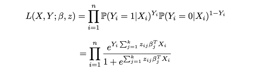
And the log-likelihood:
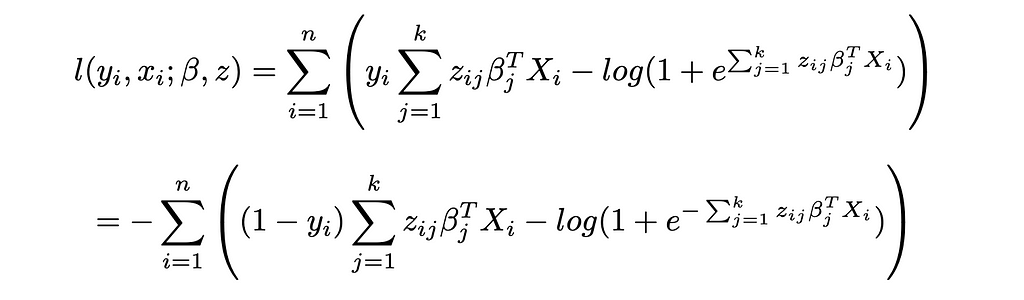
This yields the same objective function as CWC when constraining the zᵢⱼ to be binary variables.
[1] L. Baardman, I. Levin, G. Perakis, D. Singhvi, Leveraging Comparables for New Product Sales Forecasting (2018), Wiley
[2] L. Baardman, R. Cristian, G. Perakis, D. Singhvi, O. Skali Lami, L. Thayaparan, The role of optimization in some recent advances in data-driven decision-making (2023), Springer Nature
[3] D. Bertsimas, J. Dunn, Machine Learning Under a Modern Optimization Lens (2021), Dynamic Ideas
[4] G. Zeng, A comprehensive study of coefficient signs in weighted logistic regression (2024), Helyion
[5] J. Clore, K. Cios, J. DeShazo, B. Strack, Diabetes 130-US Hospitals for Years 1999–2008 [Dataset] (2014), UCI Machine Learning Repository (CC BY 4.0)
[6] R. Bock, MAGIC Gamma Telescope [Dataset] (2004), UCI Machine Learning Repository (CC BY 4.0)
[7] M. Little, Parkinsons [Dataset] (2007). UCI Machine Learning Repository (CC BY 4.0)
[8] D. Bertsimas, N. Kallus, From Predictive to Prescriptive Analytics (2019), INFORMS
Cluster While Predict: Iterative Methods for Regression and Classification was originally published in Towards Data Science on Medium, where people are continuing the conversation by highlighting and responding to this story.
Originally appeared here:
Cluster While Predict: Iterative Methods for Regression and Classification

In this article, we develop and code a Convolutional Neural Network (CNN) for a vision inspection classification task in the automotive electronics industry. Along the way, we study the concept and math of convolutional layers in depth, and we examine what CNNs actually see and which parts of the image lead them to their decisions.
Part 1: Conceptual background
Part 2: Defining and coding the CNN
Part 3: Using the trained model in production
Part 4: What did the CNN consider in its “decision”?
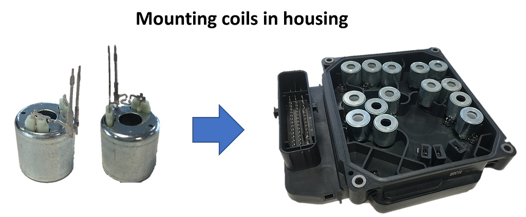
In one station of an automatic assembly line, coils with two protruding metal pins have to be positioned precisely in a housing. The metal pins are inserted into small plug sockets. In some cases, the pins are slightly bent and therefore cannot be joined by a machine. It is the task of the visual inspection to identify these coils, so that they can be sorted out automatically.
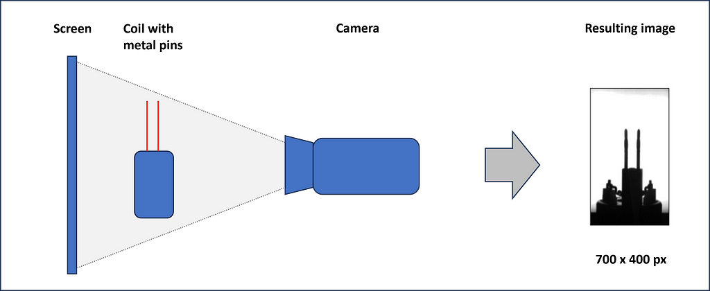
For the inspection, each coil is picked up individually and held in front of a screen. In this position, a camera takes a grayscale image. This is then examined by the CNN and classified as good or scrap.
Now, we want to define a convolutional neural network that is able to process the images and learn from pre-classified labels.
Convolutional Neural Networks are a combination of convolutional filters followed by a fully connected Neural Network (NN). CNNs are often used for image processing, like face recognition or visual inspection tasks, like in our case. Convolutional filters are matrix operations that slide over the images and recalculate each pixel of the image. We will study convolutional filters later in the article. The weights of the filters are not preset (as, e.g. the sharpen function in Photoshop) but instead are learned from the data during training.
Let’s check an example of the architecture of a CNN. For our convenience, we choose the model we will implement later.

We want to feed the CNN with our inspection images of size 400 px in height and 700 px in width. Since the images are grayscale, the corresponding PyTorch tensor is of size 1x400x700. If we used a colored image, we would have 3 incoming channels: one for red, one for green and one for blue (RGB). In this case the tensor would be 3x400x700.
The first convolutional filter has 6 kernels of size 5×5 that slide over the image and produce 6 independent new images, called feature maps, of slightly reduced size (6x396x696). The ReLU activation is not explicitly shown in Fig. 3. It does not change the dimensions of the tensors but sets all negative values to zero. ReLU is followed by the MaxPooling layer with a kernel size of 2×2. It halves the width and height of each image.
All three layers — convolution, ReLU, and MaxPooling — are implemented a second time. This finally brings us 16 feature maps with images of height 97 pixels and width 172 pixels. Next, all the matrix values are flattened and fed into the equally sized first layer of a fully connected neural network. Its second layer is already reduced to 120 neurons. The third and output layer has only 2 neurons: one represents the label “OK”, and the other the label “not OK” or “scrap”.
If you are not yet clear about the changes in the dimensions, please be patient. We study how the different kinds of layers — convolution, ReLU, and MaxPooling — work in detail and impact the tensor dimensions in the next chapters.
Convolutional filters have the task of finding typical structures/patterns in an image. Frequently used kernel sizes are 3×3 or 5×5. The 9, respectively 25, weights of the kernel are not specified upfront but learned during training (here we assume that we have only one input channel; otherwise, the number of weights multiply by input channels). The kernels slide over the matrix representation of the image (each input channel has its own kernel) with a defined stride in the horizontal and vertical directions. The corresponding values of the kernel and the matrix are multiplied and summed up. The summation results of each sliding position form the new image, which we call the feature map. We can specify multiple kernels in a convolutional layer. In this case, we receive multiple feature maps as the result. The kernel slides over the matrix from left to right and top to bottom. Therefore, Fig. 4 shows the kernel in its fifth sliding position (not counting the “…”). We see three input channels for the colors red, green, and blue (RGB). Each channel has one kernel only. In real applications, we often define multiple kernels per input channel.
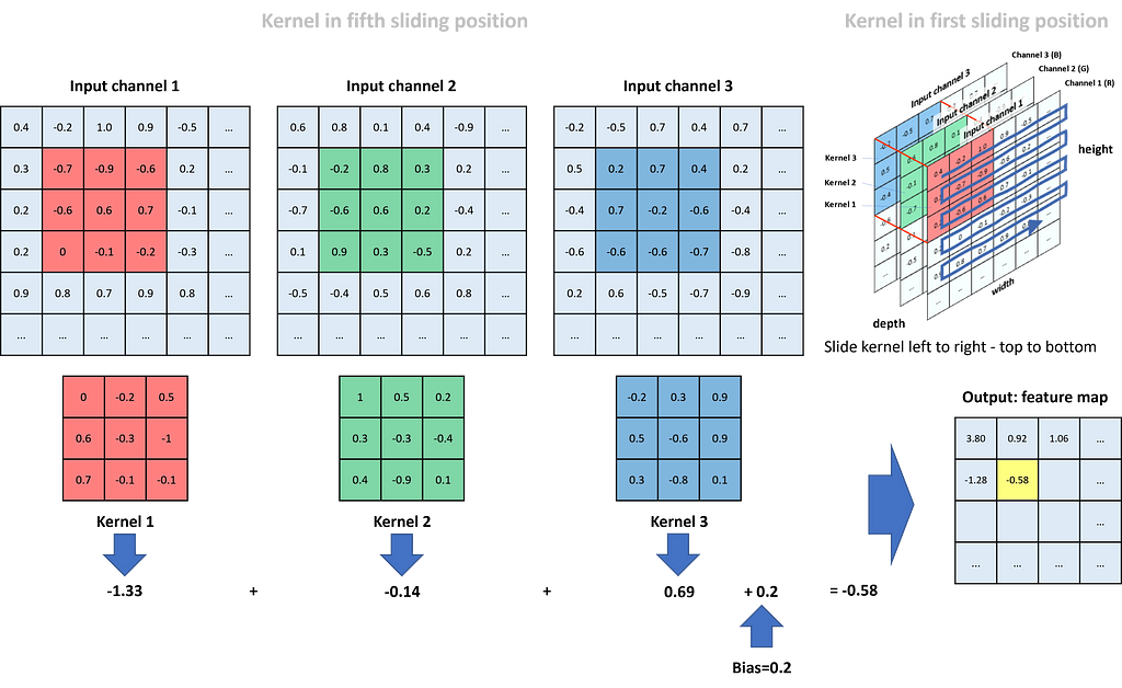
Kernel 1 does its work for the red input channel. In the shown position, we compute the respective new value in the feature map as (-0.7)*0 + (-0.9)*(-0.2) + (-0.6)*0.5 + (-0.6)*0.6 + 0.6*(-0.3) + 0.7*(-1) + 0*0.7 + (-0.1)*(-0.1) + (-0.2)*(-0.1) = (-1.33). The respective calculation for the green channel (kernel 2) adds up to -0.14, and for the blue channel (kernel 3) to 0.69. To receive the final value in the feature map for this specific sliding position, we sum up all three channel values and add a bias (bias and all kernel weights are defined during training of the CNN): (-1.33) + (-0.14) + 0.69 + 0.2 = -0.58. The value is placed in the position of the feature map highlighted in yellow.
Finally, if we compare the size of the input matrices to the size of the feature map, we see that through the kernel operations, we lost two rows in height and two columns in width.
After the convolution, the feature maps are passed through the activation layer. Activation is required to give the network nonlinear capabilities. The two most frequently used activation methods are Sigmoid and ReLU (Rectified Linear Unit). ReLU activation sets all negative values to zero while leaving positive values unchanged.
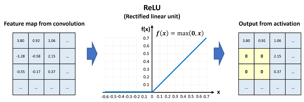
In Fig. 5, we see that the values of the feature map pass the ReLU activation element-wise.
ReLU activation has no impact on the dimensions of the feature map.
Pooling layers have mainly the task of reducing the size of the feature maps while keeping the important information for the classification. In general, we can pool by calculating the average of an area in the kernel or returning the maximum. MaxPooling is more beneficial in most applications because it reduces the noise in the data. Typical kernel sizes for pooling are 2×2 or 3×3.
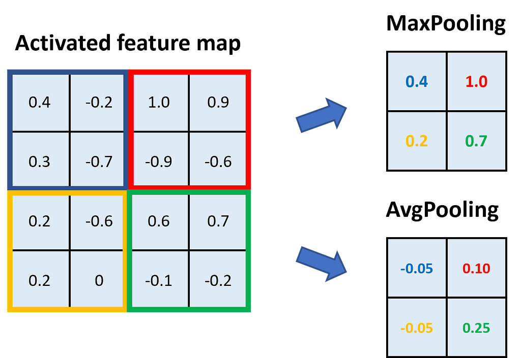
In Fig. 6, we see an example of MaxPooling and AvgPooling with a kernel size of 2×2. The feature map is divided into areas of the kernel size, and within those areas, we take either the maximum (→ MaxPooling) or the average (→ AvgPooling).
Through pooling with a kernel size of 2×2, we halve the height and width of the feature map.
Now that we have studied the convolutional filters, the ReLU activation, and the pooling, we can revise Fig. 3 and the dimensions of the tensors. We start with an image of size 400×700. Since it is grayscale, it has only 1 channel, and the corresponding tensor is of size 1x400x700. We apply 6 convolutional filters of size 5×5 with a stride of 1×1 to the image. Each filter returns its own feature map, so we receive 6 of them. Due to the larger kernel compared to Fig. 4 (5×5 instead of 3×3), this time we lose 4 columns and 4 rows in the convolution. This means the returning tensor has the size 6x396x696.
In the next step, we apply MaxPooling with a 2×2 kernel to the feature maps (each map has its own pooling kernel). As we have learned, this reduces the maps’ dimensions by a factor of 2. Accordingly, the tensor is now of size 6x198x348.
Now we apply 16 convolutional filters of size 5×5. Each of them has a kernel depth of 6, which means that each filter provides a separate layer for the 6 channels of the input tensor. Each kernel layer slides over one of the 6 input channels, as studied in Fig. 4, and the 6 returning feature maps are added up to one. So far, we considered only one convolutional filter, but we have 16 of them. That is why we receive 16 new feature maps, each 4 columns and 4 rows smaller than the input. The tensor size is now 16x194x344.
Once more, we apply MaxPooling with a kernel size of 2×2. Since this halves the feature maps, we now have a tensor size of 16x97x172.
Finally, the tensor is flattened, which means we line up all of the 16*97*172 = 266,944 values and feed them into a fully connected neural network of corresponding size.
Conceptually, we have everything we need. Now, let’s go into the industrial use case as described in chapter 1.1.
We are going to use a couple of PyTorch libraries for data loading, sampling, and the model itself. Additionally, we load matplotlib.pyplot for visualization and PIL for transforming the images.
import torch
import torch.nn as nn
from torch.utils.data import DataLoader, Dataset
from torch.utils.data.sampler import WeightedRandomSampler
from torch.utils.data import random_split
from torchvision import datasets, transforms
import matplotlib.pyplot as plt
import numpy as np
from PIL import Image
import os
import warnings
warnings.filterwarnings("ignore")
In device, we store ‘cuda’ or ‘cpu’, depending on whether or not your computer has a GPU available. minibatch_size defines how many images will be processed in one matrix operation during the training of the model. learning_rate specifies the magnitude of parameter adjustment during backpropagation, and epochs defines how often we process the whole set of training data in the training phase.
# Device configuration
device = torch.device('cuda' if torch.cuda.is_available() else 'cpu')
print(f"Using {device} device")

# Specify hyperparameters
minibatch_size = 10
learning_rate = 0.01
epochs = 60
For loading the images, we define a custom_loader. It opens the images in binary mode, crops the inner 700×400 pixels of the image, loads them into memory, and returns the loaded images. As the path to the images, we define the relative path data/Coil_Vision/01_train_val_test. Please make sure that the data is stored in your working directory. You can download the files from my Dropbox as CNN_data.zip.
# Define loader function
def custom_loader(path):
    with open(path, 'rb') as f:
        img = Image.open(f)
        img = img.crop((50, 60, 750, 460))  #Size: 700x400 px
        img.load()
        return img

# Path of images (local to accelerate loading)
path = "data/Coil_Vision/01_train_val_test"
We define the dataset as tuples consisting of the image data and the label, either 0 for scrap parts and 1 for good parts. The method datasets.ImageFolder() reads the labels out of the folder structure. We use a transform function to first load the image data to a PyTorch tensor (values between 0 and 1) and, second, normalize the data with the approximate mean of 0.5 and standard deviation of 0.5. After the transformation, the image data is roughly standard normal distributed (mean = 0, standard deviation = 1). We split the dataset randomly into 50% training data, 30% validation data, and 20% testing data.
# Transform function for loading
transform = transforms.Compose([transforms.ToTensor(),
                                transforms.Normalize((0.5), (0.5))])

# Create dataset out of folder structure
dataset = datasets.ImageFolder(path, transform=transform, loader=custom_loader)
train_set, val_set, test_set = random_split(dataset, [round(0.5*len(dataset)),
                                                      round(0.3*len(dataset)),
                                                      round(0.2*len(dataset))])
Our data is unbalanced. We have far more good samples than scrap samples. To reduce a bias towards the majority class during training, we use a WeightedRandomSampler to give higher probability to the minority class during sampling. In lbls, we store the labels of the training dataset. With np.bincount(), we count the number of 0 labels (bc[0]) and 1 labels (bc[1]). Next, we calculate probability weights for the two classes (p_nOK and p_OK) and arrange them according to the sequence in the dataset in the list lst_train. Finally, we instantiate train_sampler from WeightedRandomSampler.
# Define a sampler to balance the classes
# training dataset
lbls = [dataset[idx][1] for idx in train_set.indices]
bc = np.bincount(lbls)
p_nOK = bc.sum()/bc[0]
p_OK = bc.sum()/bc[1]
lst_train = [p_nOK if lbl==0 else p_OK for lbl in lbls]
train_sampler = WeightedRandomSampler(weights=lst_train, num_samples=len(lbls))
Lastly, we define three data loaders for the training, the validation, and the testing data. Data loaders feed the neural network with batches of datasets, each consisting of the image data and the label.
For the train_loader and the val_loader, we set the batch size to 10 and shuffle the data. The test_loader operates with shuffled data and a batch size of 1.
# Define loader with batchsize
train_loader = DataLoader(dataset=train_set, batch_size=minibatch_size, sampler=train_sampler)
val_loader = DataLoader(dataset=val_set, batch_size=minibatch_size, shuffle=True)
test_loader = DataLoader(dataset=test_set, shuffle=True)
To inspect the image data, we plot five good samples (“OK”) and five scrap samples (“nOK”). To do this, we define a matplotlib figure with 2 rows and 5 columns and share the x- and the y-axis. In the core of the code snippet, we nest two for-loops. The outer loop receives batches of data from the train_loader. Each batch consists of ten images and the corresponding labels. The inner loop enumerates the batches’ labels. In its body, we check if the label equals 0 — then we plot the image under “nOK” in the second row — or if the label equals 1 — then we plot the image under “OK” in the first row. Once count_OK and count_nOK both are greater or equal 5, we break the loop, set the title, and show the figure.
# Figure and axes object
fig, axs = plt.subplots(nrows=2, ncols=5, figsize=(20,7), sharey=True, sharex=True)

count_OK = 0
count_nOK = 0

# Loop over loader batches
for (batch_data, batch_lbls) in train_loader:

    # Loop over batch_lbls
    for i, lbl in enumerate(batch_lbls):

        # If label is 0 (nOK) plot image in row 1
        if (lbl.item() == 0) and (count_nOK < 5):
            axs[1, count_nOK].imshow(batch_data[i][0], cmap='gray')
            axs[1, count_nOK].set_title(f"nOK Part#: {str(count_nOK)}", fontsize=14)
            count_nOK += 1

        # If label is 1 (OK) plot image in row 0
        elif (lbl.item() == 1) and (count_OK < 5):
            axs[0, count_OK].imshow(batch_data[i][0], cmap='gray')
            axs[0, count_OK].set_title(f"OK Part#: {str(count_OK)}", fontsize=14)
            count_OK += 1

    # If both counters are >=5 stop looping
    if (count_OK >=5) and (count_nOK >=5):
        break

# Config the plot canvas
fig.suptitle("Sample plot of OK and nonOK Parts", fontsize=24)
plt.setp(axs, xticks=[], yticks=[])
plt.show()
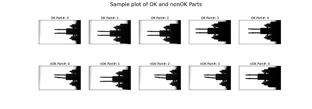
In Fig. 7, we see that most of the nOK samples are clearly bent, but a few are not really distinguishable by eye (e.g., lower right sample).
The model corresponds to the architecture depicted in Fig. 3. We feed the grayscale image (only one channel) into the first convolutional layer and define 6 kernels of size 5 (equals 5×5). The convolution is followed by a ReLU activation and a MaxPooling with a kernel size of 2 (2×2) and a stride of 2 (2×2). All three operations are repeated with the dimensions shown in Fig. 3. In the final block of the __init__() method, the 16 feature maps are flattened and fed into a linear layer of equivalent input size and 120 output nodes. It is ReLU activated and reduced to only 2 output nodes in a second linear layer.
In the forward() method, we simply call the model layers and feed in the x tensor.
class CNN(nn.Module):

    def __init__(self):
        super().__init__()

        # Define model layers
        self.model_layers = nn.Sequential(

            nn.Conv2d(in_channels=1, out_channels=6, kernel_size=5),
            nn.ReLU(),
            nn.MaxPool2d(kernel_size=2, stride=2),

            nn.Conv2d(in_channels=6, out_channels=16, kernel_size=5),
            nn.ReLU(),
            nn.MaxPool2d(kernel_size=2, stride=2),

            nn.Flatten(),
            nn.Linear(16*97*172, 120),
            nn.ReLU(),
            nn.Linear(120, 2)
        )

    def forward(self, x):
        out = self.model_layers(x)
        return out
We instantiate model from the CNN class and push it either on the CPU or on the GPU. Since we have a classification task, we choose the CrossEntropyLoss function. For managing the training process, we call the Stochastic Gradient Descent (SGD) optimizer.
# Define model on cpu or gpu
model = CNN().to(device)

# Loss and optimizer
loss = nn.CrossEntropyLoss()

optimizer = torch.optim.SGD(model.parameters(), lr=learning_rate)
To get an idea of our model’s size in terms of parameters, we iterate over model.parameters() and sum up, first, all model parameters (num_param) and, second, those parameters that will be adjusted during backpropagation (num_param_trainable). Finally, we print the result.
# Count number of parameters / thereof trainable
num_param = sum([p.numel() for p in model.parameters()])
num_param_trainable = sum([p.numel() for p in model.parameters() if p.requires_grad == True])

print(f"Our model has {num_param:,} parameters. Thereof trainable are {num_param_trainable:,}!")

The print out tells us that the model has more than 32 million parameters, thereof all trainable.
Before we start the model training, let’s prepare a function to support the validation and testing. The function val_test() expects a dataloader and the CNN model as parameters. It turns off the gradient calculation with torch.no_grad() and iterates over the dataloader. With one batch of images and labels at hand, it inputs the images into the model and determines the model’s predicted classes with output.argmax(1) over the returned logits. This method returns the indices of the largest values; in our case, this represents the class indices.
We count and sum up the correct predictions and save the image data, the predicted class, and the labels of the wrong predictions. Finally, we calculate the accuracy and return it together with the misclassified images as the function’s output.
def val_test(dataloader, model):
    # Get dataset size
    dataset_size = len(dataloader.dataset)

    # Turn off gradient calculation for validation
    with torch.no_grad():
        # Loop over dataset
        correct = 0
        wrong_preds = []
        for (images, labels) in dataloader:
            images, labels = images.to(device), labels.to(device)

            # Get raw values from model
            output = model(images)

            # Derive prediction
            y_pred = output.argmax(1)

            # Count correct classifications over all batches
            correct += (y_pred == labels).type(torch.float32).sum().item()

            # Save wrong predictions (image, pred_lbl, true_lbl)
            for i, _ in enumerate(labels):
                if y_pred[i] != labels[i]:
                    wrong_preds.append((images[i], y_pred[i], labels[i]))

        # Calculate accuracy
        acc = correct / dataset_size

    return acc, wrong_preds
The model training consists of two nested for-loops. The outer loop iterates over a defined number of epochs, and the inner loop enumerates the train_loader. The enumeration returns a batch of image data and the corresponding labels. The image data (images) is passed to the model, and we receive the model’s response logits in outputs. outputs and the true labels are passed to the loss function. Based on loss l, we perform backpropagation and update the parameter with optimizer.step. outputs is a tensor of dimension batchsize x output nodes, in our case 10 x 2. We receive the model’s prediction through the indices of the max values over the rows, either 0 or 1.
Finally, we count the number of correct predictions (n_correct), the true OK parts (n_true_OK), and the number of samples (n_samples). Each second epoch, we calculate the training accuracy, the true OK share, and call the validation function (val_test()). All three values are printed for information purpose during the training run. With the last line of code, we save the model with all its parameters in “model.pth”.
acc_train = {}
acc_val = {}
# Iterate over epochs
for epoch in range(epochs):

    n_correct=0; n_samples=0; n_true_OK=0
    for idx, (images, labels) in enumerate(train_loader):
        model.train()
        # Push data to gpu if available
        images, labels = images.to(device), labels.to(device)

        # Forward pass
        outputs = model(images)
        l = loss(outputs, labels)

        # Backward and optimize
        optimizer.zero_grad()
        l.backward()
        optimizer.step()

        # Get prediced labels (.max returns (value,index))
        _, y_pred = torch.max(outputs.data, 1)

        # Count correct classifications
        n_correct += (y_pred == labels).sum().item()
        n_true_OK += (labels == 1).sum().item()
        n_samples += labels.size(0)

    # At end of epoch: Eval accuracy and print information
    if (epoch+1) % 2 == 0:
        model.eval()
        # Calculate accuracy
        acc_train[epoch+1] = n_correct / n_samples
        true_OK = n_true_OK / n_samples
        acc_val[epoch+1] = val_test(val_loader, model)[0]

        # Print info
        print (f"Epoch [{epoch+1}/{epochs}], Loss: {l.item():.4f}")
        print(f"      Training accuracy: {acc_train[epoch+1]*100:.2f}%")
        print(f"      True OK: {true_OK*100:.3f}%")
        print(f"      Validation accuracy: {acc_val[epoch+1]*100:.2f}%")

# Save model and state_dict
torch.save(model, "model.pth")
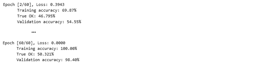
Training takes a couple of minutes on the GPU of my laptop. It is highly recommended to load the images from the local drive. Otherwise, training time might increase by orders of magnitude!
The printouts from training inform that the loss has reduced significantly, and the validation accuracy — the accuracy on data the model has not used for updating its parameters — has reached 98.4%.
An even better impression on the training progress is obtained if we plot the training and validation accuracy over the epochs. We can easily do this because we saved the values each second epoch.
We create a matplotlib figure and axes with plt.subplots() and plot the values over the keys of the accuracy dictionaries.
# Instantiate figure and axe object
fig, ax = plt.subplots(figsize=(10,6))
plt.plot(list(acc_train.keys()), list(acc_train.values()), label="training accuracy")
plt.plot(list(acc_val.keys()), list(acc_val.values()), label="validation accuracy")
plt.title("Accuracies", fontsize=24)
plt.ylabel("%", fontsize=14)
plt.xlabel("Epochs", fontsize=14)
plt.setp(ax.get_xticklabels(), fontsize=14)
plt.legend(loc='best', fontsize=14)
plt.show()
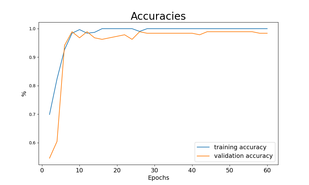
If you want to use the model for production and not only for study purpose, it is highly recommended to save and load the model with all its parameters. Saving was already part of the training code. Loading the model from your drive is equally simple.
# Read model from file
model = torch.load("model.pth")
model.eval()
Remember, we reserved another 20% of our data for testing. This data is totally new to the model and has never been loaded before. We can use this brand-new data to double-check the validation accuracy. Since the validation data has been loaded but never been used to update the model parameters, we expect a similar accuracy to the test value. To conduct the test, we call the val_test() function on the test_loader.
print(f"test accuracy: {val_test(test_loader,model)[0]*100:0.1f}%")

In the specific example, we reach a test accuracy of 99.2%, but this is highly dependent on chance (remember: random distribution of images to training, validation, and testing data).
The visualization of the misclassified images is pretty straightforward. First, we call the val_test() function. It returns a tuple with the accuracy value at index position 0 (tup[0]) and another tuple at index position 1 (tup[1]) with the image data (tup[1][0]), the predicted labels (tup[1][1]), and the true labels (tup[1][2]) of the misclassified images. In case tup[1] is not empty, we enumerate it and plot the misclassified images with appropriate headings.
%matplotlib inline

# Call test function
tup = val_test(test_loader, model)

# Check if wrong predictions occur
if len(tup[1])>=1:

    # Loop over wrongly predicted images
    for i, t in enumerate(tup[1]):
        plt.figure(figsize=(7,5))
        img, y_pred, y_true = t
        img = img.to("cpu").reshape(400, 700)
        plt.imshow(img, cmap="gray")
        plt.title(f"Image {i+1} - Predicted: {y_pred}, True: {y_true}", fontsize=24)
        plt.axis("off")
        plt.show()
        plt.close()
else:
    print("No wrong predictions!")
In our example, we have only one misclassified image, which represents 0.8% of the test dataset (we have 125 test images). The image was classified as OK but has the label nOK. Frankly, I would have misclassified it too :).
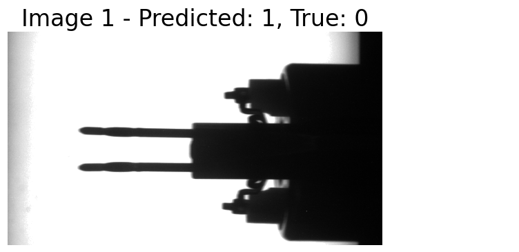
In the production phase, we assume that the CNN model is trained and the parameters are ready to be loaded. Our aim is to load new images into the model and let it classify whether the respective electronic component is good for assembly or not (see chapter 1.1 The task: Classify an industrial component as good or scrap).
We start by loading the required libraries, setting the device as ‘cuda’ or ‘cpu’, defining the class CNN (exactly as in chapter 2.8), and loading the model from file with torch.load(). We need to define the class CNN before loading the parameters; otherwise, the parameters cannot be assigned correctly.
# Load the required libraries
import torch
import torch.nn as nn
from torch.utils.data import DataLoader, Dataset
from torchvision import datasets, transforms
import matplotlib.pyplot as plt
from PIL import Image
import os

# Device configuration
device = torch.device('cuda' if torch.cuda.is_available() else 'cpu')

# Define the CNN model exactly as in chapter 2.8
class CNN(nn.Module):

    def __init__(self):
        super(CNN, self).__init__()

        # Define model layers
        self.model_layers = nn.Sequential(

            nn.Conv2d(in_channels=1, out_channels=6, kernel_size=5),
            nn.ReLU(),
            nn.MaxPool2d(kernel_size=2, stride=2),

            nn.Conv2d(in_channels=6, out_channels=16, kernel_size=5),
            nn.ReLU(),
            nn.MaxPool2d(kernel_size=2, stride=2),

            nn.Flatten(),
            nn.Linear(16*97*172, 120),
            nn.ReLU(),
            nn.Linear(120, 2),
            #nn.LogSoftmax(dim=1)
        )

    def forward(self, x):
        out = self.model_layers(x)
        return out

# Load the model's parameters
model = torch.load("model.pth")
model.eval()
With running this code snippet, we have the CNN model loaded and parameterized in our computer’s memory.
As for the training phase, we need to prepare the images for processing in the CNN model. We load them from a specified folder, crop the inner 700×400 pixels, and transform the image data to a PyTorch tensor.
# Define custom dataset
class Predict_Set(Dataset):
    def __init__(self, img_folder, transform):
        self.img_folder = img_folder
        self.transform = transform
        self.img_lst = os.listdir(self.img_folder)

    def __len__(self):
        return len(self.img_lst)

    def __getitem__(self, idx):
        img_path = os.path.join(self.img_folder, self.img_lst[idx])
        img = Image.open(img_path)
        img = img.crop((50, 60, 750, 460))  #Size: 700x400
        img.load()
        img_tensor = self.transform(img)
        return img_tensor, self.img_lst[idx]
We perform all the steps in a custom dataset class called Predict_Set(). In __init__(), we specify the image folder, accept a transform function, and load the images from the image folder into the list self.img_lst. The method __len__() returns the number of images in the image folder. __getitem__() composes the path to an image from the folder path and the image name, crops the inner part of the image (as we did for the training dataset), and applies the transform function to the image. Finally, it returns the image tensor and the image name.
The final step in data preparation is to define a data loader that allows to iterate over the images for classification. Along the way, we specify the path to the image folder and define the transform function as a pipeline that first loads the image data to a PyTorch tensor, and, second, normalizes the data to a range of approximately -1 to +1. We instantiate our custom dataset Predict_Set() to a variable predict_set and define the data loader predict_loader. Since we do not specify a batch size, predict_loader returns one image at a time.
# Path to images (preferably local to accelerate loading)
path = "data/Coil_Vision/02_predict"

# Transform function for loading
transform = transforms.Compose([transforms.ToTensor(),
                                transforms.Normalize((0.5), (0.5))])

# Create dataset as instance of custom dataset
predict_set = Predict_Set(path, transform=transform)

# Define loader
predict_loader = DataLoader(dataset=predict_set)
So far, the preparation of the image data for classification is complete. However, what we are still missing is a custom function that transfers the images to the CNN model, translates the model’s response into a classification, and returns the classification results. This is exactly what we do with predict().
def predict(dataloader, model):

    # Turn off gradient calculation
    with torch.no_grad():

        img_lst = []; y_pred_lst = []; name_lst = []
        # Loop over data loader
        for image, name in dataloader:
            img_lst.append(image)
            image = image.to(device)

            # Get raw values from model
            output = model(image)

            # Derive prediction
            y_pred = output.argmax(1)
            y_pred_lst.append(y_pred.item())
            name_lst.append(name[0])

    return img_lst, y_pred_lst, name_lst
predict() expects a data loader and the CNN model as its parameters. In its core, it iterates over the data loader, transfers the image data to the model, and interprets the models response with output.argmax(1) as the classification result — either 0 for scrap parts (nOK) or 1 for good parts (OK). The image data, the classification result, and the image name are appended to lists and the lists are returned as the function’s result.
Finally, we want to utilize our custom functions and loaders to classify new images. In the folder “data/Coil_Vision/02_predict” we have reserved four images of electronic components that wait to be inspected. Remember, we want the CNN model to tell us whether we can use the components for automatic assembly or if we need to sort them out because the pins are likely to cause problems while trying to push them in the plug sockets.
We call the custom function predict(), which returns a list of images, a list of classification results, and a list of image names. We enumerate the lists and plot the images with the names and the classification as headings.
# Predict labels for images
imgs, lbls, names  = predict(predict_loader, model)

# Iterate over classified images
for idx, image in enumerate(imgs):
    plt.figure(figsize=(8,6))
    plt.imshow(image.squeeze(), cmap="gray")
    plt.title(f"nFile: {names[idx]}, Predicted label: {lbls[idx]}", fontsize=18)
    plt.axis("off")
    plt.show()
    plt.close()
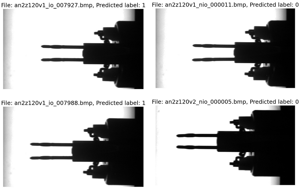
We see that the two images on the left side have been classified a good (label 1) and the two on the right as scrap (label 0). Due to our training data, the model is quite sensitive, and even small bends in the pins lead to them being classified as scrap.
We have gone deep into the details of the CNN and our industrial use case so far. This seems like a good opportunity to take one step further and try to understand what the CNN model “sees” while processing the image data. To do this, we first study the convolutional layers and then examine which parts of the image are specifically important for the classification.
To gain a better understanding of how convolutional filters work and what they do to the images, let’s examine the layers in our industrial example in more detail.
To access the layers, we enumerate model.children(), which is a generator for the model’s structure. If the layer is a convolutional layer, we append it to the list all_layers and save the weights’ dimensions in conv_weights. If we have a ReLU or a MaxPooling layer, we have no weights. In this case, we append the layer and “*” to the respective lists. Next, we enumerate all_layers, print the layer type, and the weights’ dimensions.
# Empty lists to store the layers and the weights
all_layers = []; conv_weights = []

# Iterate over the model's structure
# (First level nn.Sequential)
for _, layer in enumerate(list(model.children())[0]):
    if type(layer) == nn.Conv2d:
        all_layers.append(layer)
        conv_weights.append(layer.weight)
    elif type(layer) in [nn.ReLU, nn.MaxPool2d]:
        all_layers.append(layer)
        conv_weights.append("*")

# Print layers and dimensions of weights
for idx, layer in enumerate(all_layers):
    print(f"{idx+1}. Layer: {layer}")
    if type(layer) == nn.Conv2d:
        print(f"          weights: {conv_weights[idx].shape}")
    else:
        print(f"          weights: {conv_weights[idx]}")
    print()

Please compare the code snippet’s output with Fig. 3. The first convolutional layer has one input — the original image with only one channel — and returns six feature maps. We apply six kernels, each of depth one and size 5×5. Correspondingly, the weights are of dimension torch.Size([6, 1, 5, 5]). In contrast, layer 4 receives six feature maps as input and returns 16 maps as output. We apply 16 convolutional kernels, each of depth 6 and size 5×5. The weights’ dimension is therefore torch.Size([16, 6, 5, 5]).
Now, we know the convolutional filters’ dimensions. Next, we want to see their weights, which they have gained during the training process. Since we have so many different filters (six in the first convolutional layer and 16 in the second), we select, in both cases, the first input channel (index 0).
import itertools

# Iterate through all layers
for idx_out, layer in enumerate(all_layers):

    # If layer is a convolutional filter
    if type(layer) == nn.Conv2d:

        # Print layer name
        print(f"n{idx_out+1}. Layer: {layer} n")

        # Prepare plot and weights
        plt.figure(figsize=(25,6))
        weights = conv_weights[idx_out][:,0,:,:] # only first input channel
        weights = weights.detach().to('cpu')

        # Enumerate over filter weights (only first input channel)
        for idx_in, f in enumerate(weights):
            plt.subplot(2,8, idx_in+1)
            plt.imshow(f, cmap="gray")
            plt.title(f"Filter {idx_in+1}")

            # Print texts
            for i, j in itertools.product(range(f.shape[0]), range(f.shape[1])):
                if f[i,j] > f.mean():
                    color = 'black'
                else:
                    color = 'white'
                plt.text(j, i, format(f[i, j], '.2f'), horizontalalignment='center', verticalalignment='center', color=color)

            plt.axis("off")
        plt.show()
        plt.close()
We iterate over all_layers. If the layer is a convolutional layer (nn.Conv2d), then we print the layer’s index and the layer’s core data. Next, we prepare a plot and extract the weights matrix for the first input layer as an example. We enumerate all output layers and plot them with plt.imshow(). Finally, we print the weights’ values on the image so that we get an intuitive visualization of the convolutional filters.
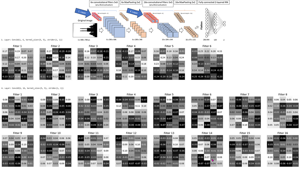
Fig. 12 shows the six convolutional filter kernels of layer 1 and the 16 kernels of layer 4 (for input channel 0). The model schematic in the upper right indicates the filters with a red outline. We see that the majority of values are close to 0, and some are in the range of positive or negative 0.20–0.25. The numbers represent the values used for the convolution demonstrated in Fig. 4. This gives us the feature maps, which we inspect next.
According to Fig. 4, we receive the first feature maps through the convolution of the input image. Therefore, we load a random image from the test_loader and push it to the CPU (in case you operate the CNN on the GPU).
# Test loader has a batch size of 1
img = next(iter(test_loader))[0].to(device)
print(f"nImage has shape: {img.shape}n")

# Plot image
img_copy = img.to('cpu')
plt.imshow(img_copy.reshape(400,700), cmap="gray")
plt.axis("off")
plt.show()
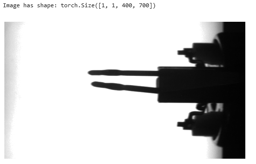
Now we pass the image data img through the first convolution layer (all_layers[0]) and save the output in results. Next, we iterate over all_layers and feed the next layer with the output from the previous layer operation. Those operations are convolutions, ReLU activations or MaxPoolings. The output of each operation we append to results.
# Pass the image through the first layer
results = [all_layers[0](img)]

# Pass the results of the previous layer to the next layer
for idx in range(1, len(all_layers)):  # Start at 1, first layer already passed!
    results.append(all_layers[idx](results[-1]))  # Pass the last result to the layer
Finally, we plot the original image, the feature maps after passing the first layer (convolution), the second layer (ReLU), the third layer (MaxPooling), the forth layer (2nd convolution), the fifth layer (2nd ReLU), and the sixth layer (2nd MaxPooling).
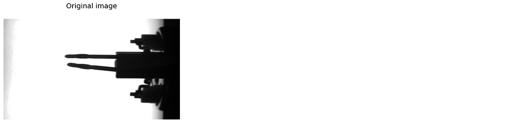
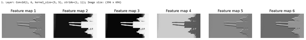
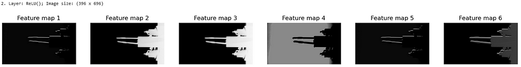
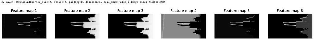
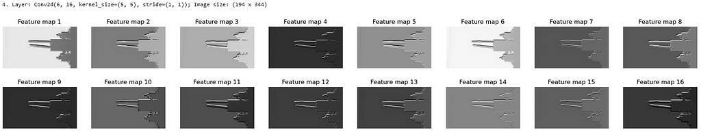
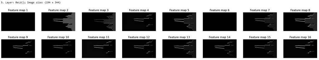

We see that the convolutional kernels (compare Fig. 12) recalculate each pixel of the image. This appears as changed grayscale values in the feature maps. Some of the feature maps are sharpened compared to the original image or have a stronger black-and-white contrast, while others seem to be faded.
The ReLU operations turn dark gray into black since negative values are set to zero.
MaxPooling keeps the images almost unchanged while halving the image size in both dimensions.
Before we finish, let’s analyze which areas of the image are particularly decisive for the classification into scrap (index 0) or good parts (index 1). For this purpose, we use Gradient-weighted Class Activation Mapping (gradCAM). This technique computes the gradients of the trained model with respect to the predicted class (the gradients show how much the inputs — the image pixels — influence the prediction). The averages of the gradients of each feature map (= output channel of convolution layer) build the weights with which the feature maps are multiplied when calculating a heat map for visualization.
But let’s look at one step after the other.
def gradCAM(x):

    # Run model and predict
    logits = model(x)
    pred = logits.max(-1)[-1] # Returns index of max value (0 or 1)

    # Fetch activations at final conv layer
    last_conv = model.model_layers[:5]
    activations = last_conv(x)

    # Compute gradients with respect to model's prediction
    model.zero_grad()
    logits[0,pred].backward(retain_graph=True)

    # Compute average gradient per output channel of last conv layer
    pooled_grads = model.model_layers[3].weight.grad.mean((1,2,3))

    # Multiply each output channel with its corresponding average gradient
    for i in range(activations.shape[1]):
        activations[:,i,:,:] *= pooled_grads[i]

    # Compute heatmap as average over all weighted output channels
    heatmap = torch.mean(activations, dim=1)[0].cpu().detach()

    return heatmap
We define a function gradCAM that expects the input data x, an image or a feature map, and returns a heatmap.
In the first block, we input x in the CNN model and receive logits, a tensor of shape [1, 2] with two values only. The values represent the predicted probabilities of the classes 0 and 1. We select the index of the larger value as the model’s prediction pred.
In the second block, we extract the first five layers of the model — from first convolution to second ReLU — and save them to last_conv. We run x through the selected layers and store the output in activations. As the name suggests, those are the activations (=feature maps) of the second convolutional layer (after ReLU activation).
In the third block, we do the backward propagation for the logit value of the predicted class logits[0,pred]. In other words, we compute all the gradients of the CNN with respect to the prediction. The gradients show how much a change in the input data — the original image pixels — impact the models output — the prediction. The result is saved in the PyTorch computational graph until we delete it with model.zero_grad().
In the fourth block, we compute the averages of the gradients over the input channel, as well as the height and width of the image or the feature maps. As a result, we receive 16 average gradients for the 16 feature maps that are returned from the second convolutional layer. We save them in pooled_grads.
In the fifth block, we iterate over the 16 feature maps returned from the second convolutional layer and weight them with the average gradients pooled_grads. This operation gives more impact to those feature maps (and their pixels) that have high importance for the prediction and vice versa. From now on, activations holds not the feature maps, but the weighted feature maps.
Finally, in the last block, we compute the heatmap as the average feature map of all activations. This is what the function gradCAM returns.
Before we can plot the image and the heatmap, we need to transform both for the overlay. Remember, the feature maps are smaller than the original picture (see chapters 1.3 and 1.7), and so is the heatmap. This is why we need the function upsampleHeatmap(). The function scales the pixel values to the range of 0 to 255 and transforms them to 8-bit integer format (required from the cv2 library). It resizes the heatmap to 400×700 px and applies a color map to both the image and heatmap. Finally, we overlay 70% heatmap and 30% image and return the composition for plotting.
import cv2

def upsampleHeatmap(map, img):
    m,M = map.min(), map.max()
    i,I = img.min(), img.max()
    map = 255 * ((map-m) / (M-m))
    img = 255 * ((img-i) / (I-i))
    map = np.uint8(map)
    img = np.uint8(img)
    map = cv2.resize(map, (700,400))
    map = cv2.applyColorMap(255-map, cv2.COLORMAP_JET)
    map = np.uint8(map)
    img = cv2.applyColorMap(255-img, cv2.COLORMAP_JET)
    img = np.uint8(img)
    map = np.uint8(map*0.7 + img*0.3)
    return map
We want to plot the original image and the heatmap overlay next to each other in one row. To do this, we iterate over the data loader predict_loader, run the gradCAM() function on the images and the upsampleHeatmap() function on the heatmap and the image. Finally, we plot the original image and the heatmap in a row with matplotlib.pyplot.
# Iterate over dataloader
for idx, (image, name) in enumerate(predict_loader):

    # Compute heatmap
    image = image.to(device)
    heatmap = gradCAM(image)
    image = image.cpu().squeeze(0).permute(1,2,0)
    heatmap = upsampleHeatmap(heatmap, image)

    # Plot images and heatmaps
    fig = plt.figure(figsize=(14,5))
    fig.suptitle(f"nFile: {names[idx]}, Predicted label: {lbls[idx]}n", fontsize=24)
    plt.subplot(1, 2, 1)
    plt.imshow(image, cmap="gray")
    plt.title(f"Image", fontsize=14)
    plt.axis("off")
    plt.subplot(1, 2, 2)
    plt.imshow(heatmap)
    plt.title(f"Heatmap", fontsize=14)
    plt.tight_layout()
    plt.axis("off")
    plt.show()
    plt.close()
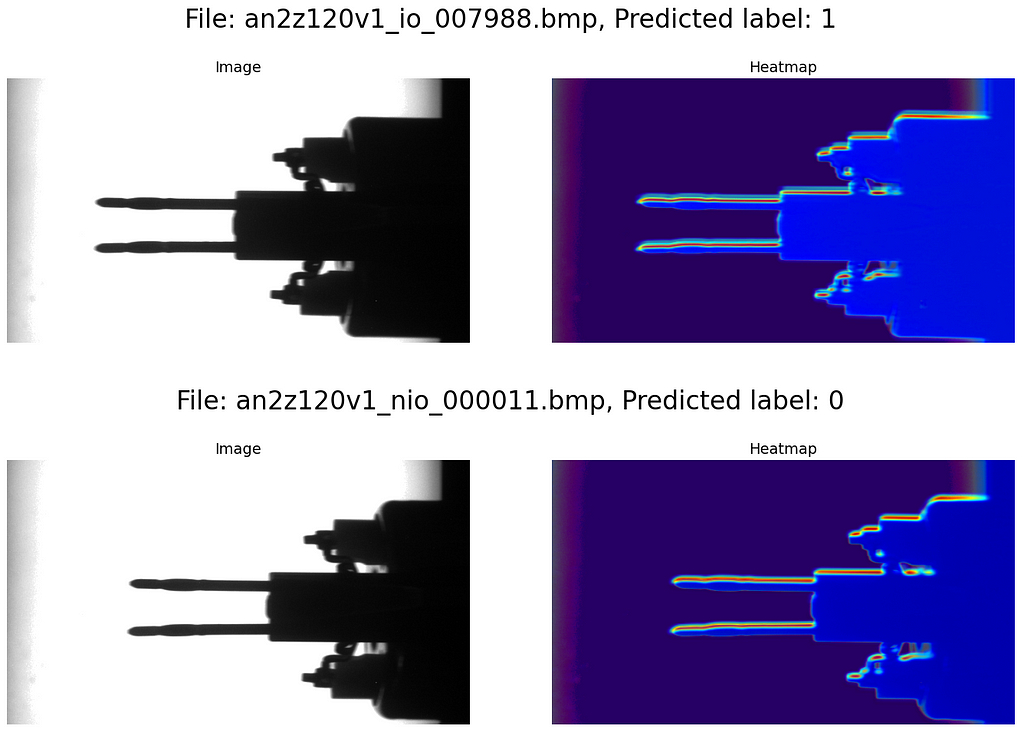
The blue areas of the heatmap have low impact on the model’s decision, while the yellow and red areas are very important. We see that in our use case, mainly the contour of the electronic component (in particular the metal pins) is decisive for the classification into scrap or good parts. Of course, this is highly reasonable, given that the use case primarily deals with bent pins.
Convolutional Neural Networks (CNNs) are nowadays a common and widely used tool for visual inspection tasks in the industrial environment. In our use case, with relatively few lines of code, we managed to define a model that classifies electronic components as good parts or scrap with high precision. The big advantage, compared to classic approaches of vision inspection, is that no process engineer needs to specify visual marks in the images for the classification. Instead, the CNN learns from labeled examples and is able to replicate this knowledge to other images. In our specific use case, 626 labeled images were sufficient for training and validation. In more complex cases, the demand for training data might be significantly higher.
Algorithms like gradCAM (Gradient-weighted Class Activation Mapping) significantly help in understanding which areas in the image are particularly relevant for the model’s decision. In this way, they support a broad use of CNNs in the industrial context by building trust in the model’s functionality.
In this article, we have explored many details of the inner workings of Convolutional Neural Networks. I hope you enjoyed the journey and have gained a deep understanding of how CNNs work.
Building a Vision Inspection CNN for an Industrial Application was originally published in Towards Data Science on Medium, where people are continuing the conversation by highlighting and responding to this story.
Originally appeared here:
Building a Vision Inspection CNN for an Industrial Application
Go Here to Read this Fast! Building a Vision Inspection CNN for an Industrial Application
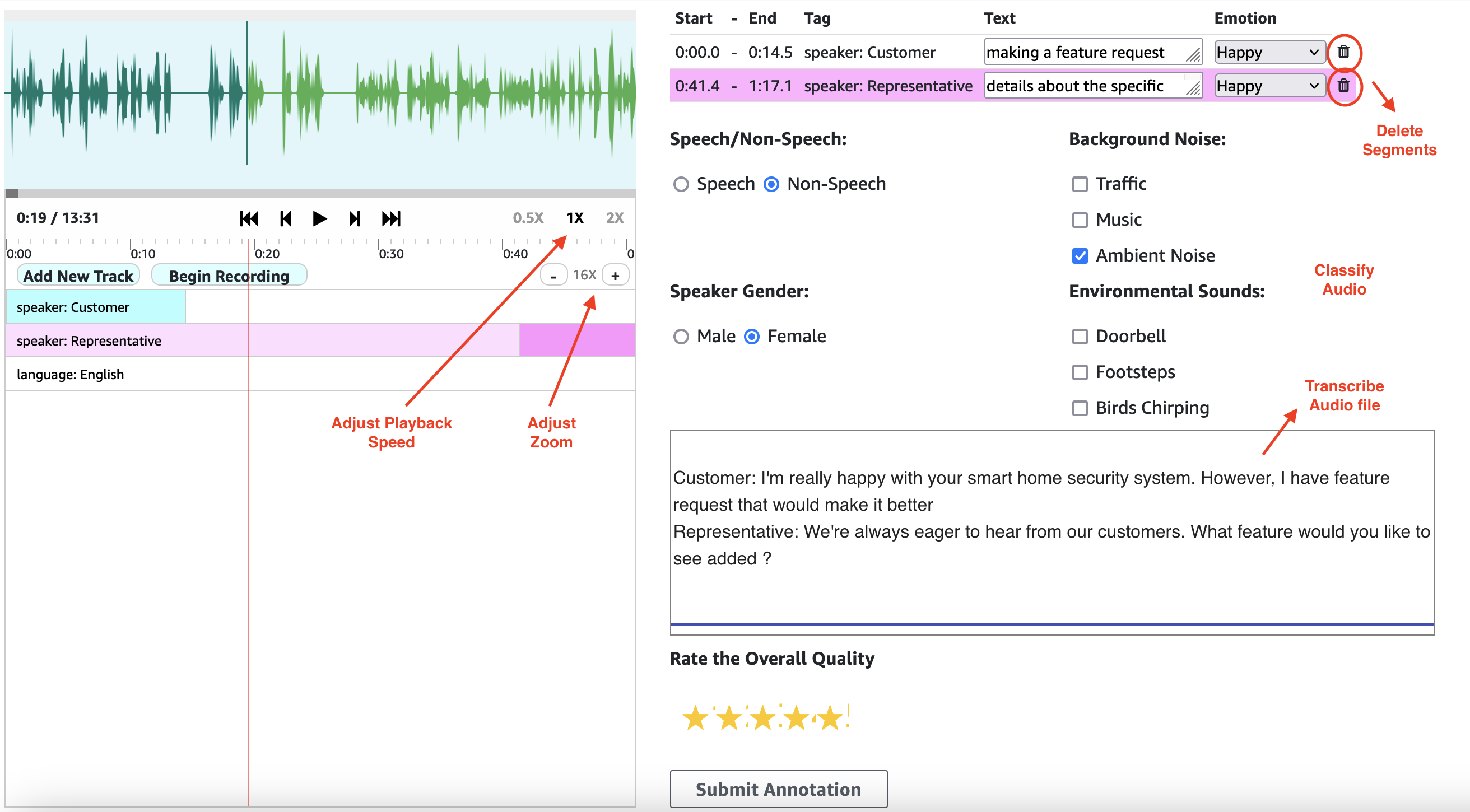

Originally appeared here:
Enhance speech synthesis and video generation models with RLHF using audio and video segmentation in Amazon SageMaker