Category: AI

This post explores how 123RF used Amazon Bedrock, Anthropic’s Claude 3 Haiku, and a vector store to efficiently translate content metadata, significantly reduce costs, and improve their global content discovery capabilities.

In this post, we explore how to integrate Amazon Q Business with SharePoint Online using the OAuth 2.0 ROPC flow authentication method. We provide both manual and automated approaches using PowerShell scripts for configuring the required Azure AD settings. Additionally, we demonstrate how to enter those details along with your SharePoint authentication credentials into the Amazon Q console to finalize the secure connection.

Today, we are excited to announce that John Snow Labs’ Medical LLM – Small and Medical LLM – Medium large language models (LLMs) are now available on Amazon SageMaker Jumpstart. For medical doctors, this tool provides a rapid understanding of a patient’s medical journey, aiding in timely and informed decision-making from extensive documentation. This summarization capability not only boosts efficiency but also makes sure that no critical details are overlooked, thereby supporting optimal patient care and enhancing healthcare outcomes.

MODEL EVALUATION & OPTIMIZATION

How underfitting and overfitting fight over your models

Every time someone builds a prediction model, they face these classic problems: underfitting and overfitting. The model cannot be too simple, yet it also cannot be too complex. The interaction between these two forces is known as the bias-variance tradeoff, and it affects every predictive model out there.

The thing about this topic of “bias-variance tradeoff” is that whenever you try to look up these terms online, you’ll find lots of articles with these perfect curves on graphs. Yes, they explain the basic idea — but they miss something important: they focus too much on theory, not enough on real-world problems, and rarely show what happens when you work with actual data.

Here, instead of theoretical examples, we’ll work with a real dataset and build actual models. Step by step, we’ll see exactly how models fail, what underfitting and overfitting look like in practice, and why finding the right balance matters. Let’s stop this fight between bias and variance, and find a fair middle ground.

What is Bias-Variance Tradeoff?

Before we start, to avoid confusion, let’s make things clear about the terms bias and variance that we are using here in machine learning. These words get used differently in many places in math and data science.

Bias can mean several things. In statistics, it means how far off our calculations are from the true answer, and in data science, it can mean unfair treatment of certain groups. Even in the for other part of machine learning which in neural networks, it’s a special number that helps the network learn

Variance also has different meanings. In statistics, it tells us how spread out numbers are from their average and in scientific experiments, it shows how much results change each time we repeat them.

But in machine learning’s “bias-variance tradeoff,” these words have special meanings.

Bias means how well a model can learn patterns. When we say a model has high bias, we mean it’s too simple and keeps making the same mistakes over and over.

Variance here means how much your model’s answers change when you give it different training data. When we say high variance, we mean the model changes its answers too much when we show it new data.

The “bias-variance tradeoff” is not something we can measure exactly with numbers. Instead, it helps us understand how our model is working: If a model has high bias, it does poorly on both training data and test data, an if a model has high variance, it does very well on training data but poorly on test data.

This helps us fix our models when they’re not working well. Let’s set up our problem and data set to see how to apply this concept.

⛳️ Setting Up Our Problem

Training and Test Dataset

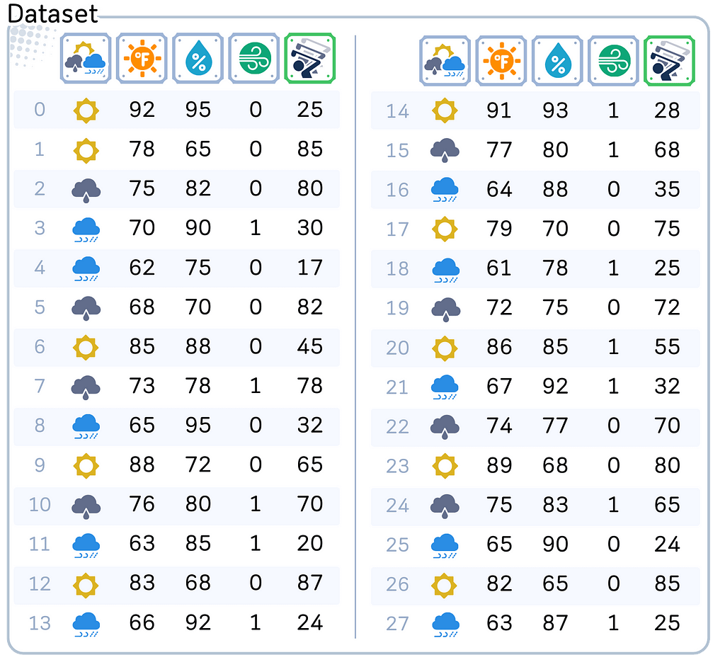
Say, you own a golf course and now you’re trying to predict how many players will show up on a given day. You have collected the data about the weather: starting from the general outlook until the details of temperature and humidity. You want to use these weather conditions to predict how many players will come.

import pandas as pd
import numpy as np
from sklearn.model_selection import train_test_split

# Data preparation
dataset_dict = {
    'Outlook': ['sunny', 'sunny', 'overcast', 'rain', 'rain', 'overcast', 'sunny', 'overcast', 'rain', 'sunny', 'overcast', 'rain', 'sunny', 'rain',
                'sunny', 'overcast', 'rain', 'sunny', 'rain', 'overcast', 'sunny', 'rain', 'overcast', 'sunny', 'overcast', 'rain', 'sunny', 'rain'],
    'Temp.': [92.0, 78.0, 75.0, 70.0, 62.0, 68.0, 85.0, 73.0, 65.0, 88.0, 76.0, 63.0, 83.0, 66.0,
              91.0, 77.0, 64.0, 79.0, 61.0, 72.0, 86.0, 67.0, 74.0, 89.0, 75.0, 65.0, 82.0, 63.0],
    'Humid.': [95.0, 65.0, 82.0, 90.0, 75.0, 70.0, 88.0, 78.0, 95.0, 72.0, 80.0, 85.0, 68.0, 92.0,
               93.0, 80.0, 88.0, 70.0, 78.0, 75.0, 85.0, 92.0, 77.0, 68.0, 83.0, 90.0, 65.0, 87.0],
    'Wind': [False, False, False, True, False, False, False, True, False, False, True, True, False, True,
             True, True, False, False, True, False, True, True, False, False, True, False, False, True],
    'Num_Players': [25, 85, 80, 30, 17, 82, 45, 78, 32, 65, 70, 20, 87, 24,
                   28, 68, 35, 75, 25, 72, 55, 32, 70, 80, 65, 24, 85, 25]
}

# Data preprocessing
df = pd.DataFrame(dataset_dict)
df = pd.get_dummies(df, columns=['Outlook'], prefix='', prefix_sep='', dtype=int)
df['Wind'] = df['Wind'].astype(int)

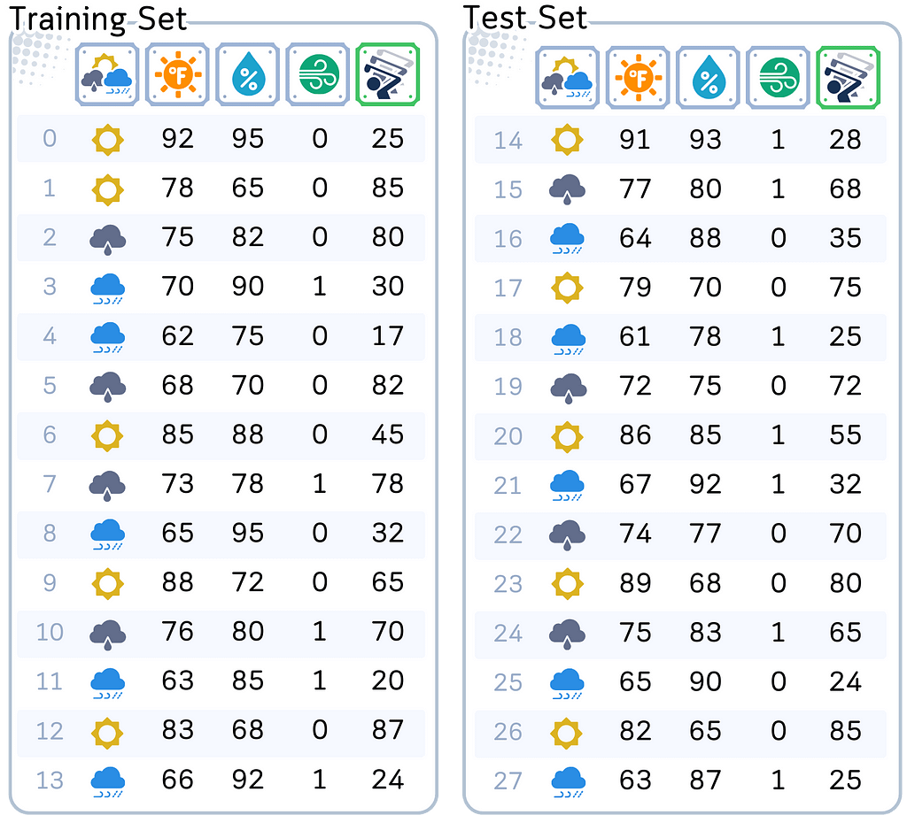
This might sound simple, but there’s a catch. We only have information from 28 different days — that’s not a lot! And to make things even trickier, we need to split this data into two parts: 14 days to help our model learn (we call this training data), and 14 days to test if our model actually works (test data).

# Split features and target
X, y = df.drop('Num_Players', axis=1), df['Num_Players']
X_train, X_test, y_train, y_test = train_test_split(X, y, train_size=0.5, shuffle=False)

Think about how hard this is. There are so many possible combination of weather conditions. It can be sunny & humid, sunny & cool, rainy & windy, overcast & cool, or other combinations. With only 14 days of training data, we definitely won’t see every possible weather combination. But our model still needs to make good predictions for any weather condition it might encounter.

This is where our challenge begins. If we make our model too simple — like only looking at temperature — it will miss important details like wind and rain. That’s not good enough. But if we make it too complex — trying to account for every tiny weather change — it might think that one random quiet day during a rainy week means rain actually brings more players. With only 14 training examples, it’s easy for our model to get confused.

And here’s the thing: unlike many examples you see online, our data isn’t perfect. Some days might have similar weather but different player counts. Maybe there was a local event that day, or maybe it was a holiday — but our weather data can’t tell us that. This is exactly what makes real-world prediction problems tricky.

So before we get into building models, take a moment to appreciate what we’re trying to do:

Using just 14 examples to create a model that can predict player counts for ANY weather condition, even ones it hasn’t seen before.

This is the kind of real challenge that makes the bias-variance trade-off so important to understand.

Model Complexity

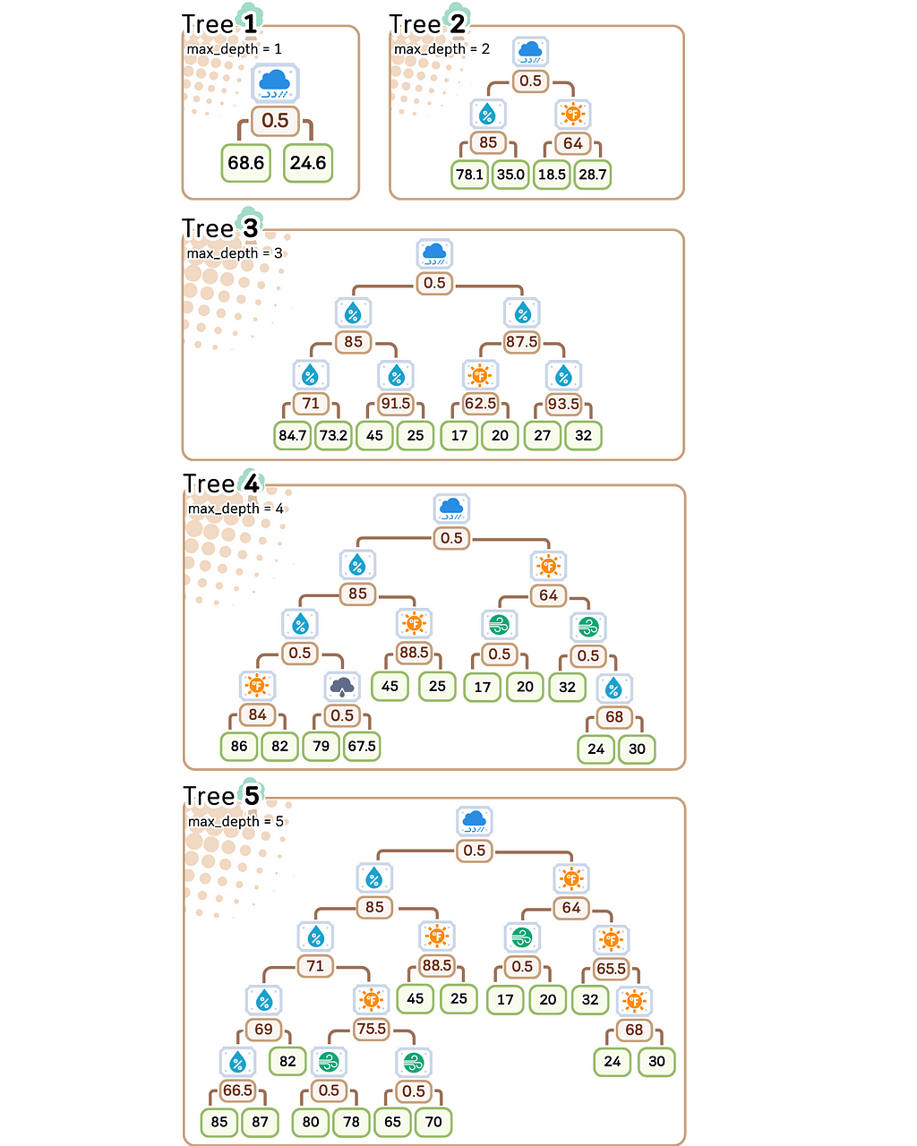
For our predictions, we’ll use decision tree regressors with varying depth (if you want to learn how this works, check out my article on decision tree basics). What matters for our discussion is how complex we let this model become.

from sklearn.tree import DecisionTreeRegressor

# Define constants
RANDOM_STATE = 3 # As regression tree can be sensitive, setting this parameter assures that we always get the same tree
MAX_DEPTH = 5

# Initialize models
trees = {depth: DecisionTreeRegressor(max_depth=depth, random_state=RANDOM_STATE).fit(X_train, y_train) 
         for depth in range(1, MAX_DEPTH + 1)}

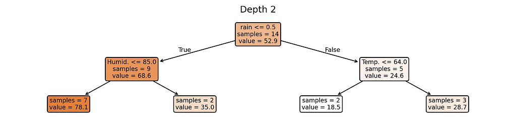
We’ll control the model’s complexity using its depth — from depth 1 (simplest) to depth 5 (most complex).

import matplotlib.pyplot as plt
from sklearn.tree import plot_tree

# Plot trees
for depth in range(1, MAX_DEPTH + 1):
    plt.figure(figsize=(12, 0.5*depth+1.5), dpi=300)
    plot_tree(trees[depth], feature_names=X_train.columns.tolist(), 
              filled=True, rounded=True, impurity=False, precision=1, fontsize=8)
    plt.title(f'Depth {depth}')
    plt.show()

Why these complexity levels matter:

• Depth 1: Extremely simple — creates just a few different predictions
• Depth 2: Slightly more flexible — can create more varied predictions
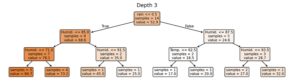
• Depth 3: Moderate complexity — getting close to too many rules
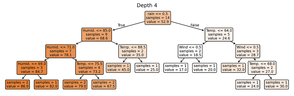
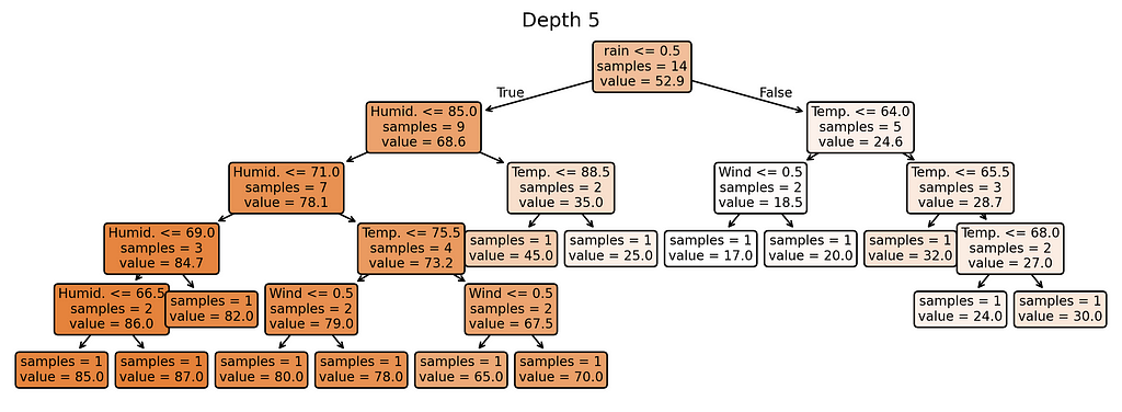
• Depth 4–5: Highest complexity — nearly one rule per training example

Notice something interesting? Our most complex model (depth 5) creates almost as many different prediction rules as we have training examples. When a model starts making unique rules for almost every training example, it’s a clear sign we’ve made it too complex for our small dataset.

Throughout the next sections, we’ll see how these different complexity levels perform on our golf course data, and why finding the right complexity is crucial for making reliable predictions.

What Makes a Model “Good”?

Prediction Errors

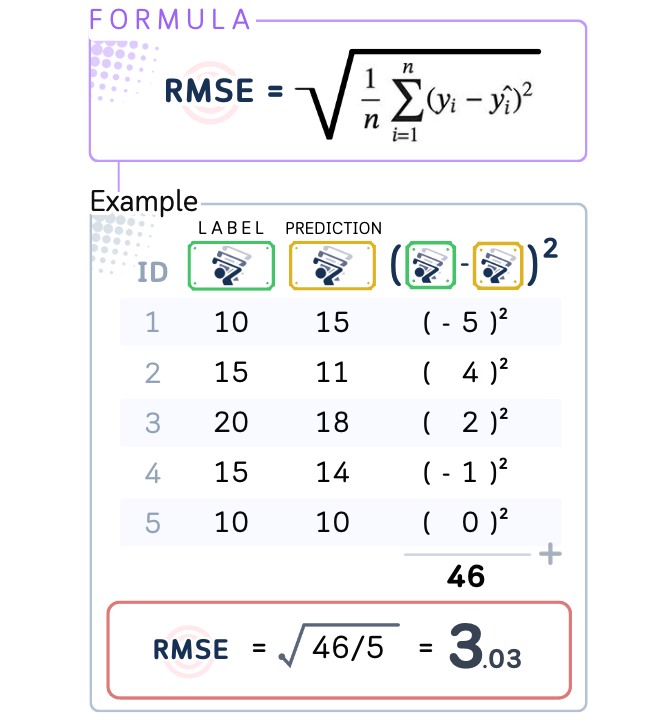
The main goal in prediction is to make guesses as close to the truth as possible. We need a way to measure errors that sees guessing too high or too low as equally bad. A prediction 10 units above the real answer is just as wrong as one 10 units below it.

This is why we use Root Mean Square Error (RMSE) as our measurement. RMSE gives us the typical size of our prediction errors. If RMSE is 7, our predictions are usually off by about 7 units. If it’s 3, we’re usually off by about 3 units. A lower RMSE means better predictions.

When measuring model performance, we always calculate two different errors. First is the training error — how well the model performs on the data it learned from. Second is the test error — how well it performs on new data it has never seen. This test error is crucial because it tells us how well our model will work in real-world situations where it faces new data.

⛳️ Looking at Our Golf Course Predictions

In our golf course case, we’re trying to predict daily player counts based on weather conditions. We have data from 28 different days, which we split into two equal parts:

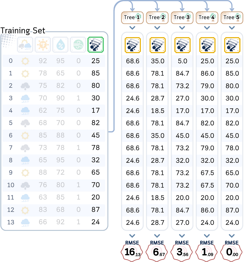
• Training data: Records from 14 days that our model uses to learn patterns
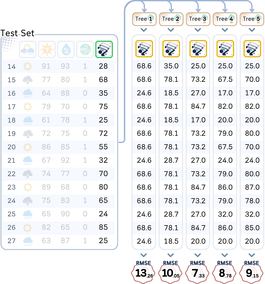
• Test data: Records from 14 different days that we keep hidden from our model

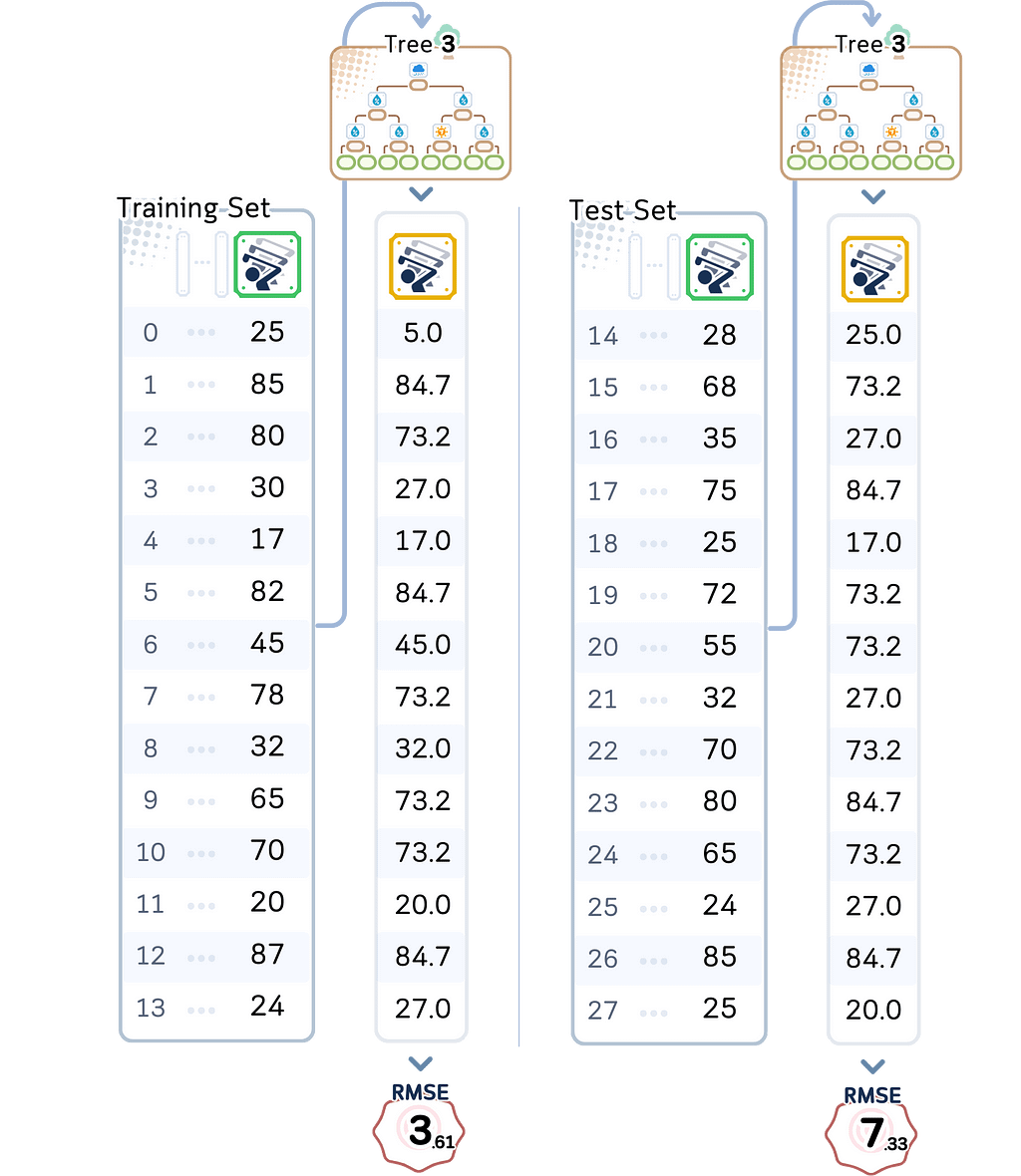
Using the models we made, let’s test both the training data and the test data, and also calculating their RMSE.

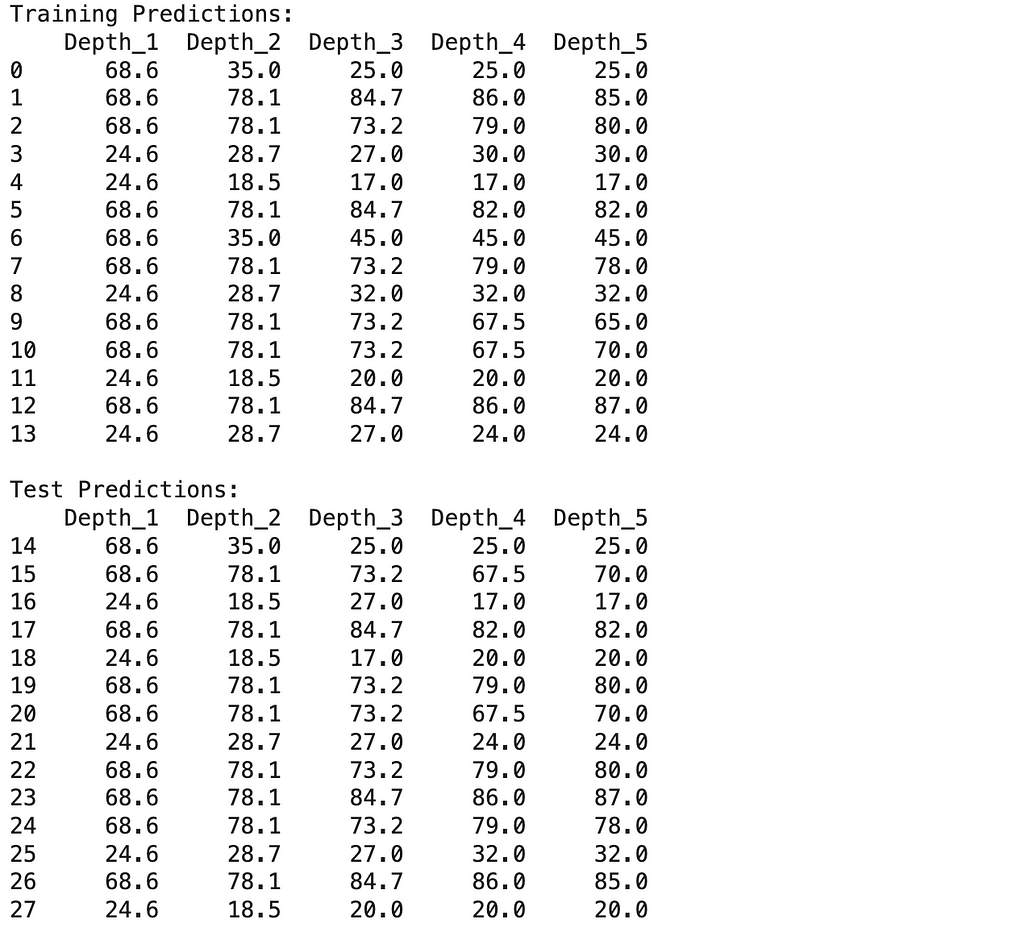
# Create training predictions DataFrame
train_predictions = pd.DataFrame({
    f'Depth_{i}': trees[i].predict(X_train) for i in range(1, MAX_DEPTH + 1)
})
#train_predictions['Actual'] = y_train.values
train_predictions.index = X_train.index

# Create test predictions DataFrame
test_predictions = pd.DataFrame({
    f'Depth_{i}': trees[i].predict(X_test) for i in range(1, MAX_DEPTH + 1)
})
#test_predictions['Actual'] = y_test.values
test_predictions.index = X_test.index

print("nTraining Predictions:")
print(train_predictions.round(1))
print("nTest Predictions:")
print(test_predictions.round(1))

from sklearn.metrics import root_mean_squared_error

# Calculate RMSE values
train_rmse = {depth: root_mean_squared_error(y_train, tree.predict(X_train))
              for depth, tree in trees.items()}
test_rmse = {depth: root_mean_squared_error(y_test, tree.predict(X_test))
             for depth, tree in trees.items()}

# Print RMSE summary as DataFrame
summary_df = pd.DataFrame({
    'Train RMSE': train_rmse.values(),
    'Test RMSE': test_rmse.values()
}, index=range(1, MAX_DEPTH + 1))
summary_df.index.name = 'max_depth'

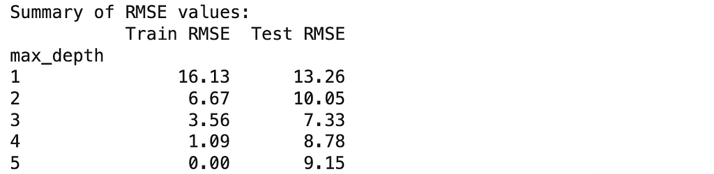
print("nSummary of RMSE values:")
print(summary_df.round(2))

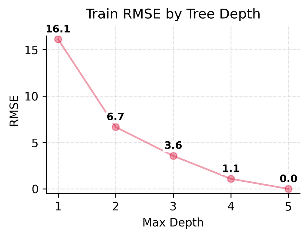
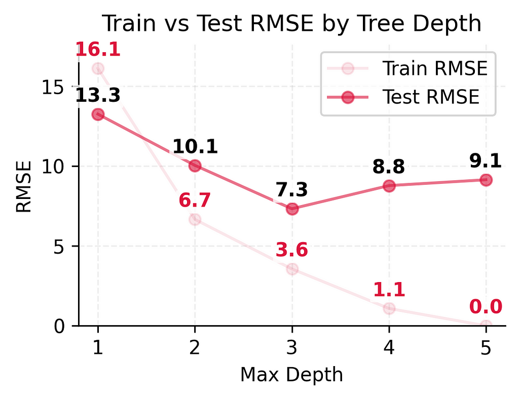
Looking at these numbers, we can already see some interesting patterns: As we make our models more complex, they get better and better at predicting player counts for days they’ve seen before — to the point where our most complex model makes perfect predictions on training data.

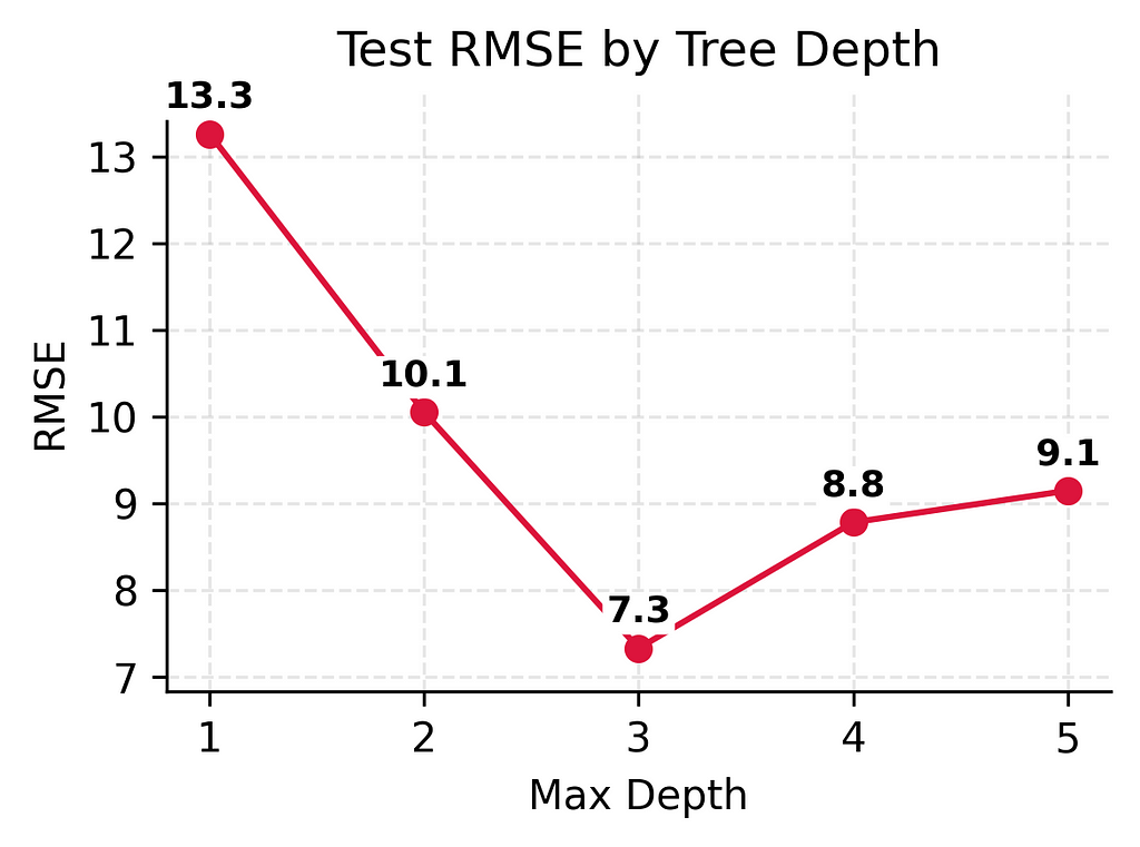
But the real test is how well they predict player counts for new days. Here, we see something different. While adding some complexity helps (the test error keeps getting better from depth 1 to depth 3), making the model too complex (depth 4–5) actually starts making things worse again.

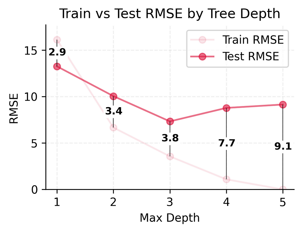
This difference between training and test performance (from being off by 3–4 players to being off by 9 players) shows a fundamental challenge in prediction: performing well on new, unseen situations is much harder than performing well on familiar ones. Even with our best performing model, we see this gap between training and test performance.

# Create figure
plt.figure(figsize=(4, 3), dpi=300)
ax = plt.gca()

# Plot main lines
plt.plot(summary_df.index, summary_df['Train RMSE'], marker='o', label='Train RMSE', 
         linestyle='-', color='crimson', alpha=0.1)
plt.plot(summary_df.index, summary_df['Test RMSE'], marker='o', label='Test RMSE', 
         linestyle='-', color='crimson', alpha=0.6)

# Add vertical lines and difference labels
for depth in summary_df.index:
    train_val = summary_df.loc[depth, 'Train RMSE']
    test_val = summary_df.loc[depth, 'Test RMSE']
    diff = abs(test_val - train_val)
    
    # Draw vertical line
    plt.vlines(x=depth, ymin=min(train_val, test_val), ymax=max(train_val, test_val), 
               colors='black', linestyles='-', lw=0.5)
    
    # Add white box behind text
    bbox_props = dict(boxstyle="round,pad=0.1", fc="white", ec="white")
    plt.text(depth - 0.15, (train_val + test_val) / 2, f'{diff:.1f}', 
             verticalalignment='center', fontsize=9, fontweight='bold',
             bbox=bbox_props)

# Customize plot
plt.xlabel('Max Depth')
plt.ylabel('RMSE')
plt.title('Train vs Test RMSE by Tree Depth')
plt.grid(True, linestyle='--', alpha=0.2)
plt.legend()

# Remove spines
ax.spines['top'].set_visible(False)
ax.spines['right'].set_visible(False)

# Set limits
plt.xlim(0.8, 5.2)
plt.ylim(0, summary_df['Train RMSE'].max() * 1.1)

plt.tight_layout()
plt.show()

Next, we’ll explore the two main ways models can fail: through consistently inaccurate predictions (bias) or through wildly inconsistent predictions (variance).

Understanding Bias (When Models Underfit)

What is Bias?

Bias happens when a model underfits the data by being too simple to capture important patterns. A model with high bias consistently makes large errors because it’s missing key relationships. Think of it as being consistently wrong in a predictable way.

When a model underfits, it shows specific behaviors:

• Similar sized errors across different predictions
• Training error is high
• Test error is also high
• Training and test errors are close to each other

High bias and underfitting are signs that our model needs to be more complex — it needs to pay attention to more patterns in the data. But how do we spot this problem? We look at both training and test errors. If both errors are high and similar to each other, we likely have a bias problem.

⛳️ Looking at Our Simple Golf Course Model

Let’s examine our simplest model’s performance (depth 1):

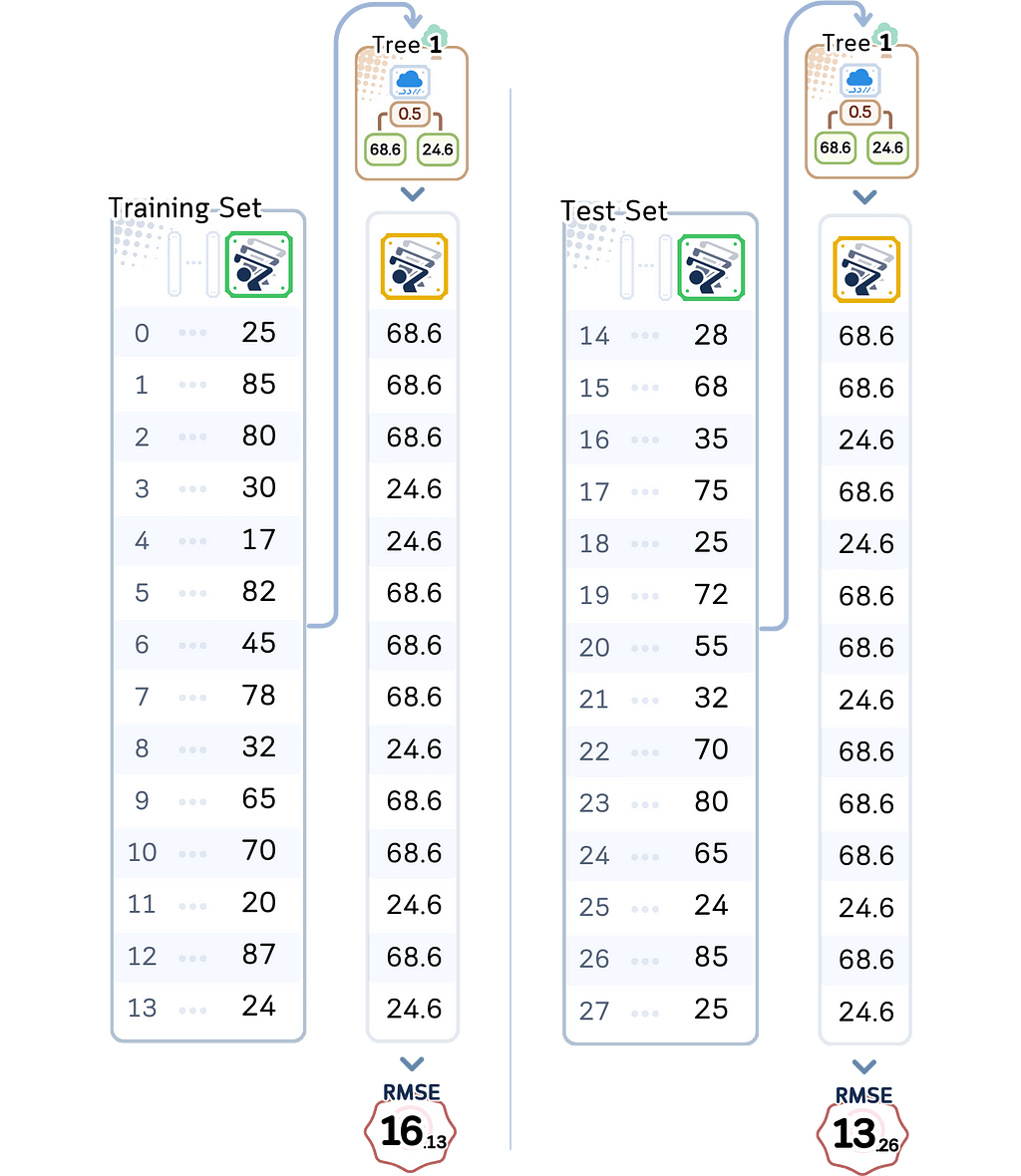
• Training RMSE: 16.13
  On average, it’s off by about 16 players even for days it trained on
• Test RMSE: 13.26
  For new days, it’s off by about 13 players

These numbers tell an important story. First, notice how high both errors are. Being off by 13–16 players is a lot when many days see between 20–80 players. Second, while the test error is higher (as we’d expect), both errors are notably large.

Looking deeper at what’s happening:

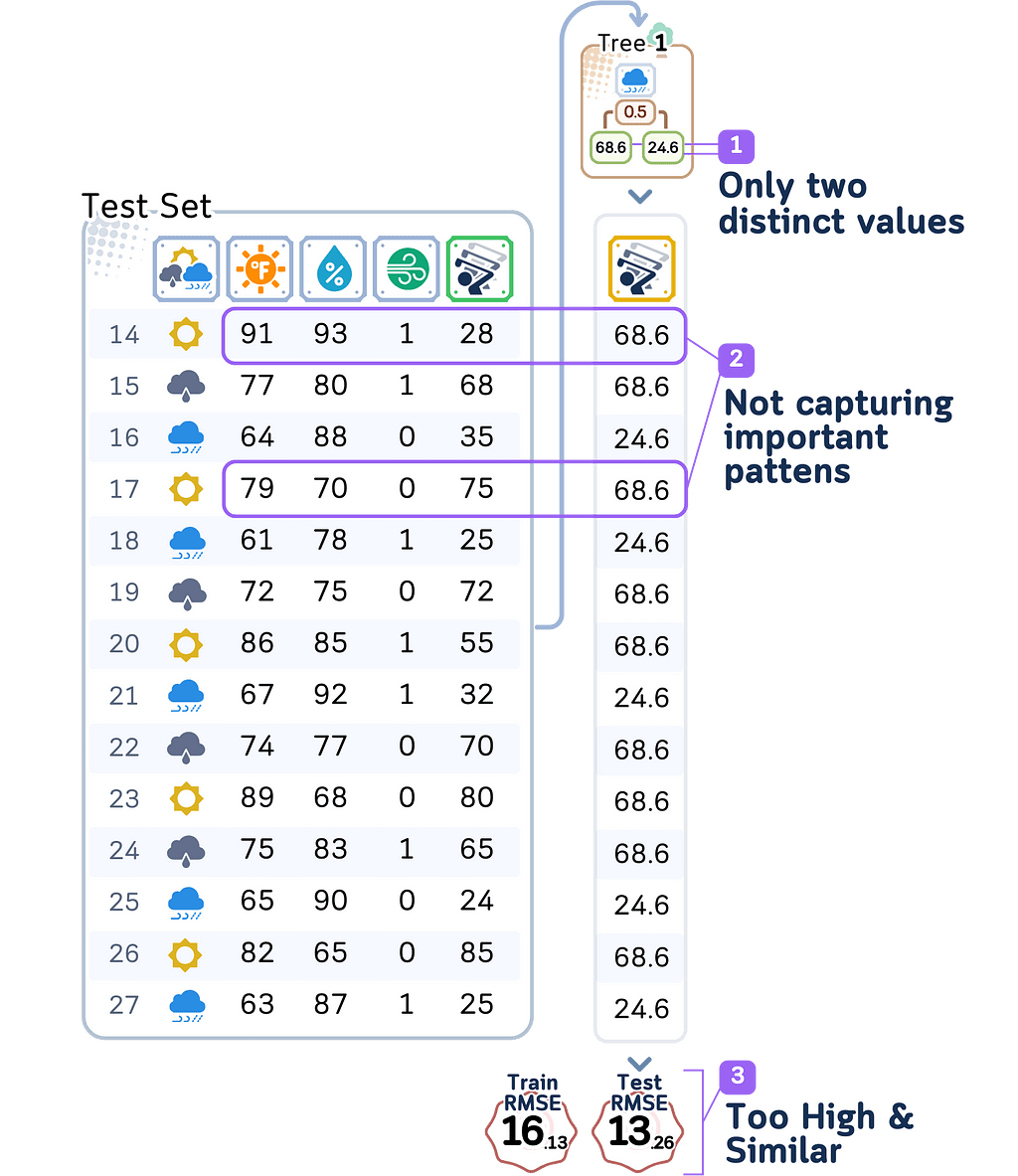
1. With depth 1, our model can only make one split decision. It might just split days based on whether it is raining or not, creating only two possible predictions for player counts. This means many different weather conditions get lumped together with the same prediction.
2. The errors follow clear patterns:
   – On hot, humid days: The model predicts too many players because it only sees whether it is raining or not
   – On cool, perfect days: The model predicts too few players because it ignores great playing conditions
3. Most telling is how similar the training and test errors are. Both are high, which means even when predicting days it trained on, the model does poorly. This is the clearest sign of high bias — the model is too simple to even capture the patterns in its training data.

This is the key problem with underfitting: the model lacks the complexity needed to capture important combinations of weather conditions that affect player turnout. Each prediction is wrong in predictable ways because the model simply can’t account for more than one weather factor at a time.

The solution seems obvious: make the model more complex so it can look at multiple weather conditions together. But as we’ll see in the next section, this creates its own problems.

Understanding Variance (When Models Overfit)

What is Variance?

Variance occurs when a model overfits by becoming too complex and overly sensitive to small changes in the data. While an underfit model ignores important patterns, an overfit model does the opposite — it treats every tiny detail as if it were an important pattern.

A model that’s overfitting shows these behaviors:

• Very small errors on training data
• Much larger errors on test data
• A big gap between training and test errors
• Predictions that change dramatically with small data changes

This problem is especially dangerous with small datasets. When we only have a few examples to learn from, an overfit model might perfectly memorize all of them without learning the true patterns that matter.

⛳️ Looking at Our Complex Golf Course Model

Let’s examine our most complex model’s performance (depth 5):

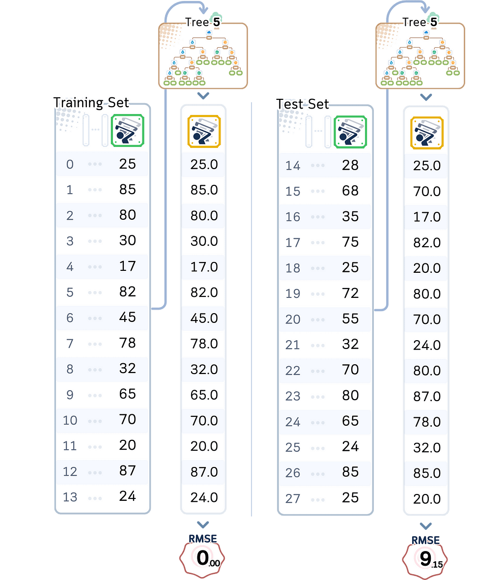
• Training RMSE: 0.00
  Perfect predictions! Not a single error on training data
• Test RMSE: 9.14
  But on new days, it’s off by about 9–10 players

These numbers reveal a classic case of overfitting. The training error of zero means our model learned to predict the exact number of players for every single day it trained on. Sounds great, right? But look at the test error — it’s much higher. This huge gap between training and test performance (from 0 to 9–10 players) is a red flag.

Looking deeper at what’s happening:

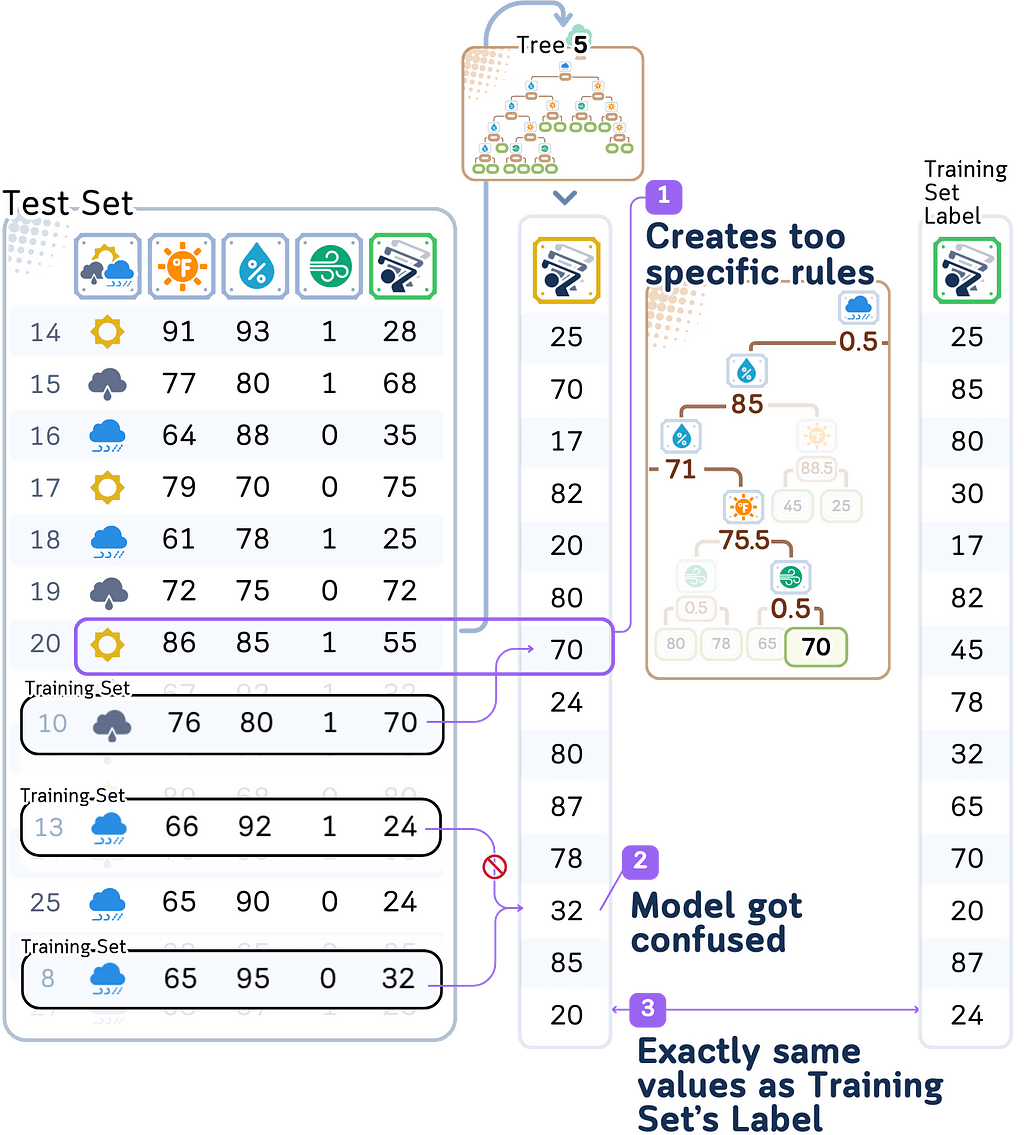
1. With depth 5, our model creates extremely specific rules. For example:
   – If it’s not rainy AND temperature is 76°F AND humidity is 80% AND it’s windy → predict exactly 70 players
   Each rule is based on just one or two days from our training data.
2. When the model sees slightly different conditions in the test data, it gets confused.
   This is very similar to our first rule above, but the model might predict a completely different number
3. With only 14 training examples, each training day gets its own highly specific set of rules. The model isn’t learning general patterns about how weather affects player counts — it’s just memorizing what happened on each specific day.

What’s particularly interesting is that while this overfit model does much better than our underfit model (test error 9.15), it’s actually worse than our moderately complex model. This shows how adding too much complexity can start hurting our predictions, even if the training performance looks perfect.

This is the fundamental challenge of overfitting: the model becomes so focused on making perfect predictions for the training data that it fails to learn the general patterns that would help it predict new situations well. It’s especially problematic when working with small datasets like ours, where creating a unique rule for each training example leaves us with no way to handle new situations reliably.

Finding the Balance

The Core Problem

Now we’ve seen both problems — underfitting and overfitting — let’s look at what happens when we try to fix them. This is where the real challenge of the bias-variance trade-off becomes clear.

Looking at our models’ performance as we made them more complex:

These numbers tell an important story. As we made our model more complex:

1. Training error kept getting better (16.3 → 6.7 → 3.6 → 1.1 → 0.0)
2. Test error improved significantly at first (13.3 → 10.1 → 7.3)
3. But then test error got slightly worse (7.3 → 8.8 → 9.1)

Why This Happens

This pattern isn’t a coincidence — it’s the fundamental nature of the bias-variance trade-off.

When we make a model more complex:

• It becomes less likely to underfit the training data (bias decreases)
• But it becomes more likely to overfit to small changes (variance increases)

Our golf course data shows this clearly:

1. The depth 1 model underfit badly — it could only split days into two groups, leading to large errors everywhere
2. Adding complexity helped — depth 2 could consider more weather combinations, and depth 3 found even better patterns
3. But depth 4 started to overfit — creating unique rules for nearly every training day

The sweet spot came with our depth 3 model:

This model is complex enough to avoid underfitting while simple enough to avoid overfitting. It has the best test performance (RMSE 7.13) of all our models.

The Real-World Impact

With our golf course predictions, this trade-off has real consequences:

• Depth 1: Underfits by only looking at temperature, missing crucial information about rain or wind
• Depth 2: Can combine two factors, like temperature AND rain
• Depth 3: Can find patterns like “warm, low humidity, and not rainy means high turnout”
• Depth 4–5: Overfits with unreliable rules like “exactly 76°F with 80% humidity on a windy day means exactly 70 players”

This is why finding the right balance matters. With just 14 training examples, every decision about model complexity has big impacts. Our depth 3 model isn’t perfect — being off by 7 players on average isn’t ideal. But it’s much better than underfitting with depth 1 (off by 13 players) or overfitting with depth 4 (giving wildly different predictions for very similar weather conditions).

How to Choose the Right Balance

The Basic Approach

When picking the best model, looking at training and test errors isn’t enough. Why? Because our test data is limited — with only 14 test examples, we might get lucky or unlucky with how well our model performs on those specific days.

A better way to test our models is called cross-validation. Instead of using just one split of training and test data, we try different splits. Each time we:

1. Pick different samples as training data
2. Train our model
3. Test on the samples we didn’t use for training
4. Record the errors

By doing this multiple times, we can understand better how well our model really works.

⛳️ What We Found With Our Golf Course Data

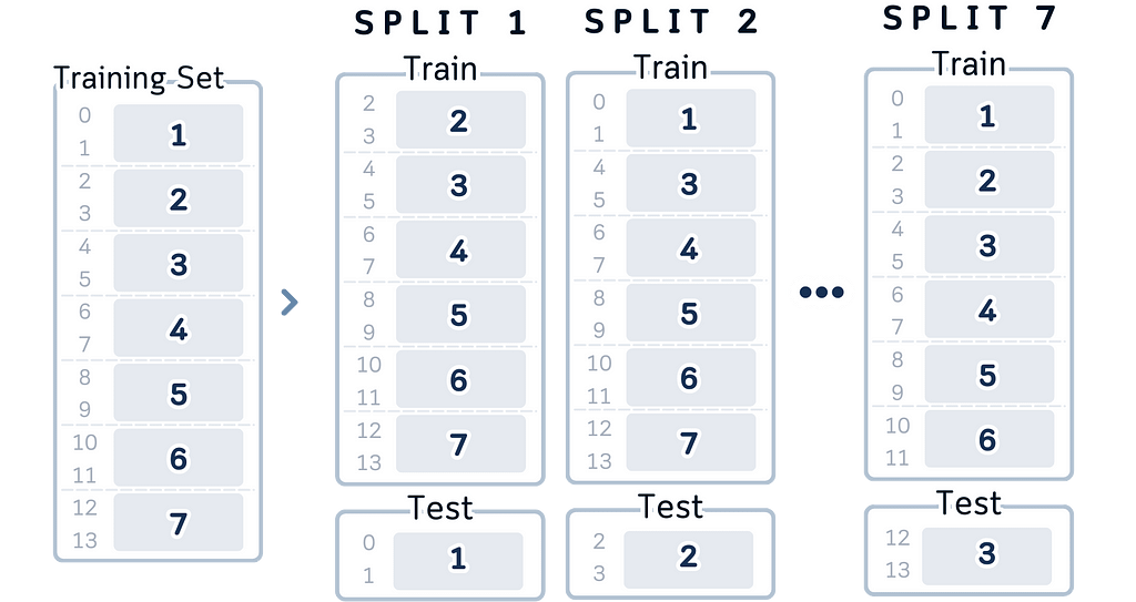
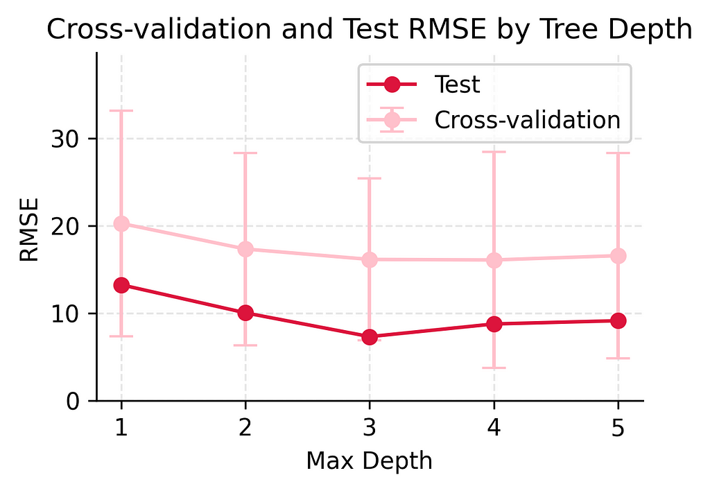
Let’s look at how our different models performed across multiple training splits using cross-validation. Given our small dataset of just 14 training examples, we used K-fold cross-validation with k=7, meaning each validation fold had 2 samples.

While this is a small validation size, it allows us to maximize our training data while still getting meaningful cross-validation estimates:

from sklearn.model_selection import KFold

def evaluate_model(X_train, y_train, X_test, y_test, n_splits=7, random_state=42):
   kf = KFold(n_splits=n_splits, shuffle=True, random_state=random_state)
   depths = range(1, 6)
   results = []
   
   for depth in depths:
       # Cross-validation scores
       cv_scores = []
       for train_idx, val_idx in kf.split(X_train):
           # Split data
           X_tr, X_val = X_train.iloc[train_idx], X_train.iloc[val_idx]
           y_tr, y_val = y_train.iloc[train_idx], y_train.iloc[val_idx]
           
           # Train and evaluate
           model = DecisionTreeRegressor(max_depth=depth, random_state=RANDOM_STATE)
           model.fit(X_tr, y_tr)
           val_pred = model.predict(X_val)
           cv_scores.append(np.sqrt(mean_squared_error(y_val, val_pred)))
       
       # Test set performance
       model = DecisionTreeRegressor(max_depth=depth, random_state=RANDOM_STATE)
       model.fit(X_train, y_train)
       test_pred = model.predict(X_test)
       test_rmse = np.sqrt(mean_squared_error(y_test, test_pred))
       
       # Store results
       results.append({
           'CV Mean RMSE': np.mean(cv_scores),
           'CV Std': np.std(cv_scores),
           'Test RMSE': test_rmse
       })
   
   return pd.DataFrame(results, index=pd.Index(depths, name='Depth')).round(2)

# Usage:
cv_df = evaluate_model(X_train, y_train, X_test, y_test)
print(cv_df)

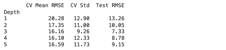
Simple Model (depth 1):
– CV Mean RMSE: 20.28 (±12.90)
– Shows high variation in cross-validation (±12.90)
– Consistently poor performance across different data splits

Slightly Flexible Model (depth 2):
– CV Mean RMSE: 17.35 (±11.00)
– Lower average error than depth 1
– Still shows considerable variation in cross-validation
– Some improvement in predictive power

Moderate Complexity Model (depth 3):
– CV Mean RMSE: 16.16 (±9.26)
– More stable cross-validation performance
– Shows good improvement over simpler models
– Best balance of stability and accuracy

Complex Model (depth 4):
– CV Mean RMSE: 16.10 (±12.33)
– Very similar mean to depth 3
– Larger variation in CV suggests less stable predictions
– Starting to show signs of overfitting

Very Complex Model (depth 5):
– CV Mean RMSE: 16.59 (±11.73)
– CV performance starts to worsen
– High variation continues
– Clear sign of overfitting beginning to occur

This cross-validation shows us something important: while our depth 3 model achieved the best test performance in our earlier analysis, the cross-validation results reveal that model performance can vary significantly. The high standard deviations (ranging from ±9.26 to ±12.90 players) across all models show that with such a small dataset, any single split of the data might give us misleading results. This is why cross-validation is so important — it helps us see the true performance of our models beyond just one lucky or unlucky split.

How to Make This Decision in Practice

Based on our results, here’s how we can find the right model balance:

1. Start Simple
   Start with the most basic model you can build. Check how well it works on both your training data and test data. If it performs poorly on both, that’s okay! It just means your model needs to be a bit more complex to capture the important patterns.
2. Gradually Add Complexity
   Now slowly make your model more sophisticated, one step at a time. Watch how the performance changes with each adjustment. When you see it starting to do worse on new data, that’s your signal to stop — you’ve found the right balance of complexity.
3. Watch for Warning Signs
   Keep an eye out for problems: If your model does extremely well on training data but poorly on new data, it’s too complex. If it does badly on all data, it’s too simple. If its performance changes a lot between different data splits, you’ve probably made it too complex.
4. Consider Your Data Size
   When you don’t have much data (like our 14 examples), keep your model simple. You can’t expect a model to make perfect predictions with very few examples to learn from. With small datasets, it’s better to have a simple model that works consistently than a complex one that’s unreliable.

Whenever we make prediction model, our goal isn’t to get perfect predictions — it’s to get reliable, useful predictions that will work well on new data. With our golf course dataset, being off by 6–7 players on average isn’t perfect, but it’s much better than being off by 11–12 players (too simple) or having wildly unreliable predictions (too complex).

Key Takeaways

Quick Ways to Spot Problems

Let’s wrap up what we’ve learned about building prediction models that actually work. Here are the key signs that tell you if your model is underfitting or overfitting:

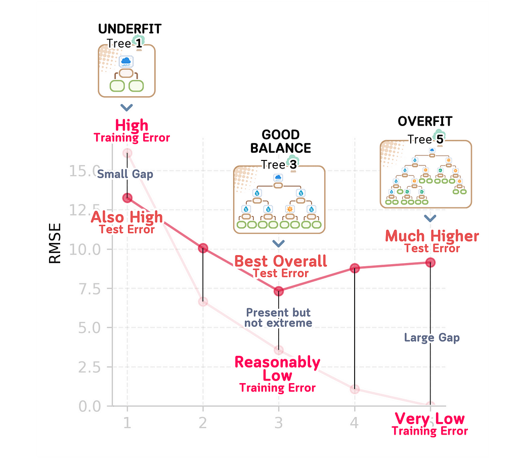
Signs of Underfitting (Too Simple):
When a model underfits, the training error will be high (like our depth 1 model’s 16.13 RMSE). Similarly, the test error will be high (13.26 RMSE). The gap between these errors is small (16.13 vs 13.26), which tells us that the model is always performing poorly. This kind of model is too simple to capture existing real relationships.

Signs of Overfitting (Too Complex):
An overfit model shows a very different pattern. You’ll see very low training error (like our depth 5 model’s 0.00 RMSE) but much higher test error (9.15 RMSE). This large gap between training and test performance (0.00 vs 9.15) is a sign that the model is easily distracted by noise in the training data and it is just memorizing the specific examples it was trained on.

Signs of a Good Balance (Like our depth 3 model):
A well-balanced model shows more promising characteristics. The training error is reasonably low (3.16 RMSE) and while the test error is higher (7.33 RMSE), it’s our best overall performance. The gap between training and test error exists but isn’t extreme (3.16 vs 7.33). This tells us the model has found the sweet spot: it’s complex enough to capture real patterns in the data while being simple enough to avoid getting distracted by noise. This balance between underfitting and overfitting is exactly what we’re looking for in a reliable model.

Final Remarks

The bias-variance trade-off isn’t just theory. It has real impacts on real predictions including in our golf course example before. The goal here isn’t to eliminate either underfitting or overfitting completely, because that’s impossible. What we want is to find the sweet spot where your model is complex enough to avoid underfitting and catch real patterns while being simple enough to avoid overfitting to random noise.

At the end, a model that’s consistently off by a little is often more useful than one that overfits — occasionally perfect but usually way off.

In the real world, reliability matters more than perfection.

---

Bias-Variance Tradeoff, Explained: A Visual Guide with Code Examples for Beginners was originally published in Towards Data Science on Medium, where people are continuing the conversation by highlighting and responding to this story.

Identify relevant subspaces: subsets of features that allow you to most effectively perform outlier detection on tabular data

This article is part of a series related to the challenges, and the techniques that may be used, to best identify outliers in data, including articles related to using PCA, Distance Metric Learning, Shared Nearest Neighbors, Frequent Patterns Outlier Factor, Counts Outlier Detector (a multi-dimensional histogram-based method), and doping. This article also contains an excerpt from my book, Outlier Detection in Python.

We look here at techniques to create, instead of a single outlier detector examining all features within a dataset, a series of smaller outlier detectors, each working with a subset of the features (referred to as subspaces).

Challenges with outlier detection

When performing outlier detection on tabular data, we’re looking for the records in the data that are the most unusual — either relative to the other records in the same dataset, or relative to previous data.

There are a number of challenges associated with finding the most meaningful outliers, particularly that there is no definition of statistically unusual that definitively specifies which anomalies in the data should be considered the strongest. As well, the outliers that are most relevant (and not necessarily the most statistically unusual) for your purposes will be specific to your project, and may evolve over time.

There are also a number of technical challenges that appear in outlier detection. Among these are the difficulties that occur where data has many features. As covered in previous articles related to Counts Outlier Detector and Shared Nearest Neighbors, where we have many features, we often face an issue known as the curse of dimensionality.

This has a number of implications for outlier detection, including that it makes distance metrics unreliable. Many outlier detection algorithms rely on calculating the distances between records — in order to identify as outliers the records that are similar to unusually few other records, and that are unusually different from most other records — that is, records that are close to few other records and far from most other records.

For example, if we have a table with 40 features, each record in the data may be viewed as a point in 40-dimensional space, and its outlierness can be evaluated by the distances from it to the other points in this space. This, then, requires a way to measure the distance between records. A variety of measures are used, with Euclidean distances being quite common (assuming the data is numeric, or is converted to numeric values). So, the outlierness of each record is often measured based on the Euclidean distance between it and the other records in the dataset.

These distance calculations can, though, break down where we are working with many features and, in fact, issues with distance metrics may appear even with only ten or twenty features, and very often with about thirty or forty or more.

We should note though, issues dealing with large numbers of features do not appear with all outlier detectors. For example, they do not tend to be significant when working with univariate tests (tests such as z-score or interquartile range tests, that consider each feature one at a time, independently of the other features — described in more detail in A Simple Example Using PCA for Outlier Detection) or when using categorical outlier detectors such as FPOF.

However, the majority of outlier detectors commonly used are numeric multi-variate outlier detectors — detectors that assume all features are numeric, and that generally work on all features at once. For example, LOF (Local Outlier Factor) and KNN (k-Nearest Neighbors) are two the the most widely-used detectors and these both evaluate the outlierness of each record based on their distances (in the high-dimensional spaces the data points live in) to the other records.

An example of outliers based on their distances to other datapoints

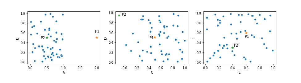
Consider the plots below. This presents a dataset with six features, shown in three 2d scatter plots. This includes two points that can reasonably be considered outliers, P1 and P2.

Looking, for now, at P1, it is far from the other points, at least in feature A. That is, considering just feature A, P1 can easily be flagged as an outlier. However, most detectors will consider the distance of each point to the other points using all six dimensions, which, unfortunately, means P1 may not necessarily stand out as an outlier, due to the nature of distance calculations in high-dimensional spaces. P1 is fairly typical in the other five features, and so it’s distance to the other points, in 6d space, may be fairly normal.

Nevertheless, we can see that this general approach to outlier detection — where we examine the distances from each record to the other records — is quite reasonable: P1 and P2 are outliers because they are far (at least in some dimensions) from the other points.

KNN and LOF algorithms

As KNN and LOF are very commonly used detectors, we’ll look at them a little closer here, and then look specifically at using subspaces with these algorithms.

With the KNN outlier detector, we pick a value for k, which determines how many neighbors each record is compared to. Let’s say we pick 10 (in practice, this would be a fairly typical value).

For each record, we then measure the distance to its 10 nearest neighbors, which provides a good sense of how isolated and remote each point is. We then need to create a single outlier score (i.e., a single number) for each record based on these 10 distances. For this, we generally then take either the mean or the maximum of these distances.

Let’s assume we take the maximum (using the mean, median, or other function works similarly, though each have their nuances). If a record has an unusually large distance to its 10th nearest neighbor, this means there are at most 9 records that are reasonably close to it (and possibly less), and that it is otherwise unusually far from most other points, so can be considered an outlier.

With the LOF outlier detector, we use a similar approach, though it works a bit differently. We also look at the distance of each point to its k nearest neighbors, but then compare this to the distances of these k neighbors to their k nearest neighbors. So LOF measures the outlierness of each point relative to the other points in their neighborhoods.

That is, while KNN uses a global standard to determine what are unusually large distances to their neighbors, LOF uses a local standard to determine what are unusually large distances.

The details of the LOF algorithm are actually a bit more involved, and the implications of the specific differences in these two algorithms (and the many variations of these algorithms) are covered in more detail in Outlier Detection in Python.

These are interesting considerations in themselves, but the main point for here is that KNN and LOF both evaluate records based on their distances to their closest neighbors. And that these distance metrics can work sub-optimally (or even completely breakdown) if using many features at once, which is reduced greatly by working with small numbers of features (subspaces) at a time.

The idea of using subspaces is useful even where the detector used does not use distance metrics, but where detectors based on distance calculations are used, some of the benefits of using subspaces can be a bit more clear. And, using distances in ways similar to KNN and LOF is quite common among detectors. As well as KNN and LOF, for example, Radius, ODIN, INFLO, and LoOP detectors, as well as detectors based on sampling, and detectors based on clustering, all use distances.

However, issues with the curse of dimensionality can occur with other detectors as well. For example, ABOD (Angle-based Outlier Detector) uses the angles between records to evaluate the outlierness of each record, as opposed to the distances. But, the idea is similar, and using subspaces can also be helpful when working with ABOD.

As well, other benefits of subspaces I’ll go through below apply equally to many detectors, whether using distance calculations or not. Still, the curse of dimensionality is a serious concern in outlier detection: where detectors use distance calculations (or similar measures, such as angle calculations), and there are many features, these distance calculations can break down. In the plots above, P1 and P2 may be detected well considering only six dimensions, and quite possibly if using 10 or 20 features, but if there were, say, 100 dimensions, the distances between all points would actually end up about the same, and P1 and P2 would not stand out at all as unusual.

Issues with moderate numbers of features

Outside of the issues related to working with very large numbers of features, our attempts to identify the most unusual records in a dataset can be undermined even when working with fairly small numbers of features.

While very large numbers of features can make the distances calculated between records meaningless, even moderate numbers of features can make records that are unusual in just one or two features more difficult to identify.

Consider again the scatter plot shown earlier, repeated here. Point P1 is an outlier in feature A (thought not in the other five features). Point P2 is unusual in features C and D, but not in the other four features). However, when considering the Euclidean distances of these points to the other points in 6-dimensional space, they may not reliably stand out as outliers. The same would be true using Manhattan, and most other distance metrics as well.

P1, for example, even in the 2d space shown in the left-most plot, is not unusually far from most other points. It’s unusual that there are no other points near it (which KNN and LOF will detect), but the distance from P1 to the other points in this 2d space is not unusual: it’s similar to the distances between most other pairs of points.

Using a KNN algorithm, we would likely be able to detect this, at least if k is set fairly low, for example, to 5 or 10 — most records have their 5th (and their 10th) nearest neighbors much closer than P1 does. Though, when including all six features in the calculations, this is much less clear than when viewing just feature A, or just the left-most plot, with just features A and B.

Point P2 stands out well as an outlier when considering just features C and D. Using a KNN detector with a k value of, say, 5, we can identify its 5 nearest neighbors, and the distances to these would be larger than is typical for points in this dataset.

Using an LOF detector, again with a k value of, say, 5, we can compare the distances to P1’s or P2’s 5 nearest neighbors to the distances to their 5 nearest neighbors and here as well, the distance from P1 or P2 to their 5 nearest neighbors would be found to be unusually large.

At least this is straightforward when considering only Features A and B, or Features C and D, but again, when considering the full 6-d space, they become more difficult to identify as outliers.

While many outlier detectors may still be able to identify P1 and P2 even with six, or a small number more, dimensions, it is clearly easier and more reliable to use fewer features. To detect P1, we really only need to consider feature A; and to identify P2, we really only need to consider features C and D. Including other features in the process simply makes this more difficult.

This is actually a common theme with outlier detection. We often have many features in the datasets we work with, and each can be useful. For example, if we have a table with 50 features, it may be that all 50 features are relevant: either a rare value in any of these features would be interesting, or a rare combination of values in two or more features, for each of these 50 features, would be interesting. It would be, then, worth keeping all 50 features for analysis.

But, to identify any one anomaly, we generally need only a small number of features. In fact, it’s very rare for a record to be unusual in all features. And it’s very rare for a record to have a anomaly based on a rare combination of many features (see Counts Outlier Detector for more explanation of this).

Any given outlier will likely have a rare value in one or two features, or a rare combination of values in a pair, or a set of perhaps three or four features. Only these features are necessary to identify the anomalies in that row, even though the other features may be necessary to detect the anomalies in other rows.

Subspaces

To address these issues, an important technique in outlier detection is using subspaces. The term subspaces simply refers to subsets of the features. In the example above, if we use the subspaces: A-B, C-D, E-F, A-E, B-C, B-D-F, and A-B-E, then we have seven subspaces (five 2d subspaces and two 3d subspaces). Creating these, we would run one (or more) detectors on each subspace, so would run at least seven detectors on each record.

Realistically, subspaces become more useful where we have many more features that six, and generally even the the subspaces themselves will have more than six features, and not just two or three, but viewing this simple case, for now, with a small number of small subspaces is fairly easy to understand.

Using these subspaces, we can more reliably find P1 and P2 as outliers. P1 would likely be scored high by the detector running on features A-B, the detector running on features A-E, and the detector running on features A-B-E. P2 would likely be detected by the detector running on features C-D, and possibly the detector running on B-C.

However, we have to be careful: using only these seven subspaces, as opposed to a single 6d space covering all features, would miss any rare combinations of, for example, A and D, or C and E. These may or may not be detected using a detector covering all six features, but definitely could not be detected using a suite of detectors that simply never examine these combinations of features.

Using subspaces does have some large benefits, but does have some risk of missing relevant outliers. We’ll cover some techniques to generate subspaces below that mitigate this issue, but it can be useful to still run one or more outlier detectors on the full dataspace as well. In general, with outlier detection, we’re rarely able to find the full set of outliers we’re interested in unless we apply many techniques. As important as the use of subspaces can be, it is still often useful to use a variety of techniques, which may include running some detectors on the full data.

Similarly, with each subspace, we may execute multiple detectors. For example, we may use both a KNN and LOF detector, as well as Radius, ABOD, and possibly a number of other detectors — again, using multiple techniques allows us to better cover the range of outliers we wish to detect.

Further Motivations for Subspaces

We’ve seen, then, a couple motivations for working with subspaces: we can mitigate the curse of dimensionality, and we can reduce where anomalies are not identified reliably where they are based on small numbers of features that are lost among many features.

As well as handling situations like this, there are a number of other advantages to using subspaces with outlier detection. These include:

• Accuracy due to the effects of using ensembles — Using multiple subspaces allows us to create ensembles (collections of outlier detectors), which allows us to combine the results of many detectors. In general, using ensembles of detectors provides greater accuracy than using a single detector. This is similar (though with some real differences too) to the way ensembles of predictors tend to be stronger for classification and regression problems than a single predictor. Here, using subspaces, each record is examined multiple times, which provides a more stable evaluation of each record than any single detector would.
• Interpretability — The results can be more interpretable, and interpretability is often a key concern in outlier detection. Very often in outlier detection, we’re flagging unusual records with the idea that they may be a concern, or a point of interest, in some way, and often they will be manually examined. Knowing why they are unusual is necessary to be able to do this efficiently and effectively. Manually assessing outliers that are flagged by detectors that examined many features can be especially difficult; on the other hand, outliers flagged by detectors using only a small number of features can be much more manageable to asses.
• Faster systems — Using fewer features allows us to create faster (and less memory-intensive) detectors. This can speed up both fitting and inference, particularly when working with detectors whose execution time is non-linear in the number of features (many detectors are, for example, quadratic in execution time based on the number of features). Depending on the detectors, using, say, 20 detectors, each covering 8 features, may actually execute faster than a single detector covering 100 features.
• Execution in parallel — Given that we use many small detectors instead of one large detector, it’s possible to execute both the fitting and the predicting steps in parallel, allowing for faster execution where there are the hardware resources to support this.
• Ease of tuning over time — Using many simple detectors creates a system that’s easier to tune over time. Very often with outlier detection, we’re simply evaluating a single dataset and wish just to identify the outliers in this. But it’s also very common to execute outlier detection systems on a long-running basis, for example, monitoring industrial processes, website activity, financial transactions, the data being input to machine learning systems or other software applications, the output of these systems, and so on. In these cases, we generally wish to improve the outlier detection system over time, allowing us to focus better on the more relevant outliers. Having a suite of simple detectors, each based on a small number of features, makes this much more manageable. It allows us to, over time, increase the weight of the more useful detectors and decrease the weight of the less useful detectors.

Choosing the subspaces

As indicated, we will need, for each dataset evaluated, to determine the appropriate subspaces. It can, though, be difficult to find the relevant set of subspaces, or at least to find the optimal set of subspaces. That is, assuming we are interested in finding any unusual combinations of values, it can be difficult to know which sets of features will contain the most relevant of the unusual combinations.

As an example, if a dataset has 100 features, we may train 10 models, each covering 10 features. We may use, say, the first 10 features for the first detector, the second set of 10 features for the second, and so on, If the first two features have some rows with anomalous combinations of values, we will detect this. But if there are anomalous combinations related to the first feature and any of the 90 features not covered by the same model, we will miss these.

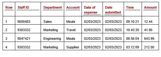
We can improve the odds of putting relevant features together by using many more subspaces, but it can be difficult to ensure all sets of features that should be together are actually together at least once, particularly where there are relevant outliers in the data that are based on three, four, or more features — which must appear together in at least one subspace to be detected. For example, in a table of staff expenses, you may wish to identify expenses for rare combinations of Department, Expense Type, and Amount. If so, these three features must appear together in at least one subspace.

So, we have the questions of how many features should be in each subspace, which features should go together, and how many subspaces to create.

There are a very large number of combinations to consider. If there are 20 features, there are ²²⁰ possible subspaces, which is just over a million. If there are 30 features, there over a billion. If we decide ahead of time how many features will be in each subspace, the numbers of combinations decreases, but is still very large. If there are 20 features and we wish to use subspaces with 8 features each, there are 20 chose 8, or 125,970 combinations. If there are 30 features and we wish for subspaces with 7 features each, there are 30 chose 7, or 2,035,800 combinations.

One approach we may wish to take is to keep the subspaces small, which allows for greater interpretability. The most interpretable option, using two features per subspace, also allows for simple visualization. However, if we have d features, we will need d*(d-1)/2 models to cover all combinations, which can be intractable. With 100 features, we would require 4,950 detectors. We usually need to use at least several features per detector, though not necessarily a large number.

We wish to use enough detectors, and enough features per detector, that each pair of features appears together ideally at least once, and few enough features per detector that the detectors have largely different features from each other. For example, if each detector used 90 out of the 100 features, we’d cover all combinations of features well, but the subspaces would still be quite large (undoing much of the benefit of using subspaces), and all the subspaces will be quite similar to each other (undoing much of the benefit of creating ensembles).

While the number of features per subspace requires balancing these concerns, the number of subspaces created is a bit more straightforward: in terms of accuracy, using more subspaces is strictly better, but is computationally more expensive.

There are a few broad approaches to finding useful subspaces. I list these here quickly, then look at some in more detail below.

• Based on domain knowledge — Here we consider which sets of features could potentially have combinations of values we would consider noteworthy.
• Based on associations — Unusual combinations of values are only possible if a set of features are associated in some way. In prediction problems, we often wish to minimize the correlations between features, but with outlier detection, these are the features that are most useful to consider together. The features with the strongest associations will have the most meaningful outliers if there are exceptions to the normal patterns.
• Based on finding very sparse regions — Records are typically considered as outliers if they are unlike most other records in the data, which implies they are located in sparse regions of the data. Therefore, useful subspaces can be found as those that contain large, nearly-empty regions.
• Randomly — This is the method used by a technique shown later called FeatureBagging and, while it can be suboptimal, it avoids the expensive searches for associations and sparse regions, and can work reasonably well where many subspaces are used.
• Exhaustive searches — This is the method employed by Counts Outlier Detector. This is limited to subspaces with small numbers of features, but the results are highly interpretable. It also avoids any computation, or biases, associated with selecting only a subset of the possible subspaces.
• Using the features related to any known outliers — If we have a set of known outliers, can identify why they are outliers (the relevant features), and are in a situation where we do not wish to identify unknown outliers (only these specific outliers), then we can take advantage of this and identify the sets of features relevant for each known outlier, and construct models for the various sets of features required.

We’ll look at a few of these next in a little more detail.

Domain knowledge

Let’s take the example of a dataset, specifically an expenses table, shown below. If examining this table, we may be able to determine the types of outliers we would and would not be interested in. Unusual combinations of Account and Amount, as well as unusual combinations of Department and Account, may be of interest; whereas Date of Expense and Time would likely not be a useful combination. We can continue in this way, creating a small number of subspaces, each with likely two, three, or four features, which can allow for very efficient and interpretable outlier detection, flagging the most relevant outliers.

This can miss cases where we have an association in the data, though the association is not obvious. So, as well as taking advantage of domain knowledge, it may be worth searching the data for associations. We can discover relationships among the features, for example, testing where features can be predicted accurately from the other features using simple predictive models. Where we find such associations, these can be worth investigating.

Discovering these associations, though, may be useful for some purposes, but may or may not be useful for the outlier detection process. If there is, for example, a relationship between accounts and the time of the day, this may simply be due to the process people happen to typically use to submit their expenses, and it may be that deviations from this are of interest, but more likely they are not.

Random feature subspaces

Creating subspaces randomly can be effective if there is no domain knowledge to draw on. This is fast and can create a set of subspaces that will tend to catch the strongest outliers, though it can miss some important outliers too.

The code below provides an example of one method to create a set of random subspaces. This example uses a set of eight features, named A through H, and creates a set of subspaces of these.

Each subspace starts by selecting the feature that is so far the least-used (if there is a tie, one is selected randomly). It uses a variable called ft_used_counts to track this. It then adds features to this subspace one at a time, each step selecting the feature that has appeared in other subspaces the least often with the features so far in the subspace. It uses a feature called ft_pair_mtx to track how many subspaces each pair of features have appeared in together so far. Doing this, we create a set of subspaces that matches each pair of features roughly equally often.

import pandas as pd
import numpy as np

def get_random_subspaces(features_arr, num_base_detectors,
                         num_feats_per_detector):
    num_feats = len(features_arr)
    feat_sets_arr = []
    ft_used_counts = np.zeros(num_feats) 
    ft_pair_mtx = np.zeros((num_feats, num_feats))  

    # Each loop generates one subspace, which is one set of features
    for _ in range(num_base_detectors):  
        # Get the set of features with the minimum count      
        min_count = ft_used_counts.min() 
        idxs = np.where(ft_used_counts == min_count)[0]    

        # Pick one of these randomly and add to the current set
        feat_set = [np.random.choice(idxs)]   

        # Find the remaining set of features
        while len(feat_set) < num_feats_per_detector: 
            mtx_with_set = ft_pair_mtx[:, feat_set]
            sums = mtx_with_set.sum(axis=1)
            min_sum = sums.min()
            min_idxs = np.where(sums==min_sum)[0]
            new_feat = np.random.choice(min_idxs)
            feat_set.append(new_feat)
            feat_set = list(set(feat_set))
            
            # Updates ft_pair_mtx
            for c in feat_set: 
                ft_pair_mtx[c][new_feat] += 1
                ft_pair_mtx[new_feat][c] += 1
            
        # Updates ft_used_counts
        for c in feat_set: 
            ft_used_counts[c] += 1

        feat_sets_arr.append(feat_set)

    return feat_sets_arr

np.random.seed(0)
features_arr = ['A', 'B', 'C', 'D', 'E', 'F', 'G', 'H'] 
num_base_detectors = 4
num_feats_per_detector = 5

feat_sets_arr = get_random_subspaces(features_arr, 
                                     num_base_detectors, 
                                     num_feats_per_detector)
for feat_set in feat_sets_arr:    
    print([features_arr[x] for x in feat_set])

Normally we would create many more base detectors (each subspace often corresponds to one base detector, though we can also run multiple base detectors on each subspace) than we do in this example, but this uses just four to keep things simple. This will output the following subspaces:

['A', 'E', 'F', 'G', 'H']
['B', 'C', 'D', 'F', 'H']
['A', 'B', 'C', 'D', 'E']
['B', 'D', 'E', 'F', 'G']

The code here will create the subspaces such that all have the same number of features. There is also an advantage in having the subspaces cover different numbers of features, as this can introduce some more diversity (which is important when creating ensembles), but there is strong diversity in any case from using different features (so long as each uses a relatively small number of features, such that the subspaces are largely different features).

Having the same number of features has a couple benefits. It simplifies tuning the models, as many parameters used by outlier detectors depend on the number of features. If all subspaces have the same number of features, they can also use the same parameters.

It also simplifies combining the scores, as the detectors will be more comparable to each other. If using different numbers of features, this can produce scores that are on different scales, and not easily comparable. For example, with k-Nearest Neighbors (KNN), we expect greater distances between neighbors if there are more features.

Feature subspaces based on correlations

Everything else equal, in creating the subspaces, it’s useful to keep associated features together as much as possible. In the code below, we provide an example of code to select subspaces based on correlations.

There are several ways to test for associations. We can create predictive models to attempt to predict each feature from each other single feature (this will capture even relatively complex relationships between features). With numeric features, the simplest method is likely to check for Spearman correlations, which will miss nonmonotonic relationships, but will detect most strong relationships. This is what is used in the code example below.

To execute the code, we first specify the number of subspaces desired and the number of features in each.

This executes by first finding all pairwise correlations between the features and storing this in a matrix. We then create the first subspace, starting by finding the largest correlation in the correlation matrix (this adds two features to this subspace) and then looping over the number of other features to be added to this subspace. For each, we take the largest correlation in the correlation matrix for any pair of features, such that one feature is currently in the subspace and one is not. Once this subspace has a sufficient number of features, we create the next subspace, taking the largest correlation remaining in the correlation matrix, and so on.

For this example, we use a real dataset, the baseball dataset from OpenML (available with a public license). The dataset turns out to contain some large correlations. The correlation, for example, between At bats and Runs is 0.94, indicating that any values that deviate significantly from this pattern would likely be outliers.

import pandas as pd
import numpy as np
from sklearn.datasets import fetch_openml

# Function to find the pair of features remaining in the matrix with the 
# highest correlation
def get_highest_corr(): 
    return np.unravel_index(
        np.argmax(corr_matrix.values, axis=None), 
        corr_matrix.shape)

def get_correlated_subspaces(corr_matrix, num_base_detectors, 
                                num_feats_per_detector):
    sets = []

    # Loop through each subspace to be created
    for _ in range(num_base_detectors): 
        m1, m2 = get_highest_corr()

        # Start each subspace as the two remaining features with 
        # the highest correlation
        curr_set = [m1, m2] 
        for _ in range(2, num_feats_per_detector):
            # Get the other remaining correlations
            m = np.unravel_index(np.argsort(corr_matrix.values, axis=None), 
                                 corr_matrix.shape) 
            m0 = m[0][::-1]
            m1 = m[1][::-1]
            for i in range(len(m0)):
                d0 = m0[i]
                d1 = m1[i]
                # Add the pair if either feature is already in the subset
                if (d0 in curr_set) or (d1 in curr_set): 
                    curr_set.append(d0)
                    curr_set = list(set(curr_set))
                    if len(curr_set) < num_feats_per_detector:
                        curr_set.append(d1)
                        # Remove duplicates
                        curr_set = list(set(curr_set)) 
                if len(curr_set) >= num_feats_per_detector:
                    break

            # Update the correlation matrix, removing the features now used 
            # in the current subspace
            for i in curr_set: 
                i_idx = corr_matrix.index[i]
                for j in curr_set:
                    j_idx = corr_matrix.columns[j]
                    corr_matrix.loc[i_idx, j_idx] = 0
            if len(curr_set) >= num_feats_per_detector:
                break

        sets.append(curr_set)
    return sets

data = fetch_openml('baseball', version=1)
df = pd.DataFrame(data.data, columns=data.feature_names)

corr_matrix = abs(df.corr(method='spearman'))
corr_matrix = corr_matrix.where(
    np.triu(np.ones(corr_matrix.shape), k=1).astype(np.bool))
corr_matrix = corr_matrix.fillna(0)

feat_sets_arr = get_correlated_subspaces(corr_matrix, num_base_detectors=5, 
                                         num_feats_per_detector=4)
for feat_set in feat_sets_arr:    
    print([df.columns[x] for x in feat_set])

This produces:

['Games_played', 'At_bats', 'Runs', 'Hits']
['RBIs', 'At_bats', 'Hits', 'Doubles']
['RBIs', 'Games_played', 'Runs', 'Doubles']
['Walks', 'Runs', 'Games_played', 'Triples']
['RBIs', 'Strikeouts', 'Slugging_pct', 'Home_runs']

PyOD

PyOD is likely the most comprehensive and well-used tool for outlier detection on numeric tabular data available in Python today. It includes a large number of detectors, ranging from very simple to very complex — including several deep learning-based methods.

Now that we have an idea of how subspaces work with outlier detection, we’ll look at two tools provided by PyOD that work with subspaces, called SOD and FeatureBagging. Both of these tools identify a set of subspaces, execute a detector on each subspace, and combine the results for a single score for each record.

Whether using subspaces or not, it’s necessary to determine what base detectors to use. If not using subspaces, we would select one or more detectors and run these on the full dataset. And, if we are using subspaces, we again select one or more detectors, here running these on each subspace. As indicated above, LOF and KNN can be reasonable choices, but PyOD provides a number of others as well that can work well if executed on each subspace, including, for example, Angle-based Outlier Detector (ABOD), models based on Gaussian Mixture Models (GMMs), Kernel Density Estimations (KDE), and several others. Other detectors, provided outside PyOD can work very effectively as well.

SOD (Subspace Outlier Detection)

SOD was designed specifically to handle situations such as shown in the scatter plots above. SOD works, similar to KNN and LOF, by identifying a neighborhood of k neighbors for each point, known as the reference set. The reference set is found in a different way, though, using a method called shared nearest neighbors (SNN).

Shared nearest neighbors are described thoroughly in this article, but the general idea is that if two points are generated by the same mechanism, they will tend to not only be close, but also to have many of the same neighbors. And so, the similarity of any two records can be measured by the number of shared neighbors they have. Given this, neighborhoods can be identified by using not only the sets of points with the smallest Euclidean distances between them (as KNN and LOF do), but the points with the most shared neighbors. This tends to be robust even in high dimensions and even where there are many irrelevant features: the rank order of neighbors tends to remain meaningful even in these cases, and so the set of nearest neighbors can be reliably found even where specific distances cannot.

Once we have the reference set, we use this to determine the subspace, which here is the set of features that explain the greatest amount of variance for the reference set. Once we identify these subspaces, SOD examines the distances of each point to the data center.

I provide a quick example using SOD below. This assumes pyod has been installed, which requires running:

pip install pyod

We’ll use, as an example, a synthetic dataset, which allows us to experiment with the data and model hyperparameters to get a better sense of the strengths and limitations of each detector. The code here provides an example of working with 35 features, where two features (features 8 and 9) are correlated and the other features are irrelevant. A single outlier is created as an unusual combination of the two correlated features.

SOD is able to identify the one known outlier as the top outlier. I set the contamination rate to 0.01 to specify to return (given there are 100 records) only a single outlier. Testing this beyond 35 features, though, SOD scores this point much lower. This example specifies the size of the reference set to be 3; different results may be seen with different values.

import pandas as pd
import numpy as np
from pyod.models.sod import SOD

np.random.seed(0)
d = np.random.randn(100, 35)
d = pd.DataFrame(d)

#A Ensure features 8 and 9 are correlated, while all others are irrelevant
d[9] = d[9] + d[8] 

# Insert a single outlier
d.loc[99, 8] = 3.5 
d.loc[99, 9] = -3.8

#C Execute SOD, flagging only 1 outlier
clf = SOD(ref_set=3, contamination=0.01) 
d['SOD Scores'] = clf.fit (d)
d['SOD Scores'] = clf.labels_

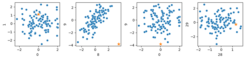
We display four scatterplots below, showing four pairs of the 35 features. The known outlier is shown as a star in each of these. We can see features 8 and 9 (the two relevant features) in the second pane, and we can see the point is a clear outlier, though it is typical in all other dimensions.

FeatureBagging

FeatureBagging was designed to solve the same problem as SOD, though takes a different approach to determining the subspaces. It creates the subspaces completely randomly (so slightly differently than the example above, which keeps a record of how often each pair of features are placed in a subspace together and attempts to balance this). It also subsamples the rows for each base detector, which provides a little more diversity between the detectors.

A specified number of base detectors are used (10 by default, though it is preferable to use more), each of which selects a random set of rows and features. For each, the maximum number of features that may be selected is specified as a parameter, defaulting to all. So, for each base detector, FeatureBagging:

• Determines the number of features to use, up to the specified maximum.
• Chooses this many features randomly.
• Chooses a set of rows randomly. This is a bootstrap sample of the same size as the number of rows.
• Creates an LOF detector (by default; other base detectors may be used) to evaluate the subspace.

Once this is complete, each row will have been scored by each base detector and the scores must then be combined into a single, final score for each row. PyOD’s FeatureBagging provides two options for this: using the maximum score and using the mean score.

As we saw in the scatter plots above, points can be strong outliers in some subspaces and not in others, and averaging in their scores from the subspaces where they are typical can water down their scores and defeat the benefit of using subspaces. In other forms of ensembling with outlier detection, using the mean can work well, but when working with multiple subspaces, using the maximum will typically be the better of the two options. Doing that, we give each record a score based on the subspace where it was most unusual. This isn’t perfect either, and there can be better options, but using the maximum is simple and is almost always preferable to the mean.

Any detector can be used within the subspaces. PyOD uses LOF by default, as did the original paper describing FeatureBagging. LOF is a strong detector and a sensible choice, though you may find better results with other base detectors.

In the original paper, subspaces are created randomly, each using between d/2 and d — 1 features, where d is the total number of features. Some researchers have pointed out that the number of features used in the original paper is likely much larger than is appropriate.

If the full number of features is large, using over half the features at once will allow the curse of dimensionality to take effect. And using many features in each detector will result in the detectors being correlated with each other (for example, if all base detectors use 90% of the features, they will use roughly the same features and tend to score each record roughly the same), which can also remove much of the benefit of creating ensembles.

PyOD allows setting the number of features used in each subspace, and it should be typically set fairly low, with a large number of base estimators created.

Using other detectors

In this article we’ve looked at subspaces as a way to improve outlier detection in a number of ways, including reducing the curse of dimensionality, increasing interpretability, allowing parallel execution, allowing easier tuning over time, and so on. Each of these are important considerations, and using subspaces is often very helpful.

There are, though, often other approaches as well that can be used for these purposes, sometimes as alternatives, and sometimes in combination of with the use of subspaces. For example, to improve interpretability, its important to, as much as possible, select model types that are inherently interpretable (for example univariate tests such as z-score tests, Counts Outlier Detector, or a detector provided by PyOD called ECOD).

Where the main interest is in reducing the curse of dimensionality, here again, it can be useful to look at model types that scale to many features well, for instance Isolation Forest or Counts Outlier Detector. It can also be useful to look at executing univariate tests, or applying PCA.

Ongoing outlier detection projects

One thing to be aware of when constructing subspaces, if they are formed based on correlations, or on sparse regions, is that the relevant subspaces may change over time as the data changes. New associations may emerge between features and new sparse regions may form that will be useful for identifying outliers, though these will be missed if the subspaces are not recalculated from time to time. Finding the relevant subspaces in these ways can be quite effective, but they may need to to be updated on some schedule, or where the data is known to have changed.

Conclusions

It’s common with outlier detection projects on tabular data for it to be worth looking at using subspaces, particularly where we have many features. Using subspaces is a relatively straightforward technique with a number of noteworthy advantages.

Where you face issues related to large data volumes, execution times, or memory limits, using PCA may also be a useful technique, and may work better in some cases than creating sub-spaces, though working with sub-spaces (and so, working with the original features, and not the components created by PCA) can be substantially more interpretable, and interpretability is often quite important with outlier detection.

Subspaces can be used in combination with other techniques to improve outlier detection. As an example, using subspaces can be combined with other ways to create ensembles: it’s possible to create larger ensembles using both subspaces (where different detectors in the ensemble use different features) as well as different model types, different training rows, different pre-processing, and so on. This can provide some further benefits, though with some increase in computation as well.

All images by author

---

Perform outlier detection more effectively using subsets of features was originally published in Towards Data Science on Medium, where people are continuing the conversation by highlighting and responding to this story.