Sometimes a Shallow Abstraction is more Valuable than Performance
Originally appeared here:
Use Tablib to Handle Simple Tabular Data in Python
Go Here to Read this Fast! Use Tablib to Handle Simple Tabular Data in Python
Sometimes a Shallow Abstraction is more Valuable than Performance
Originally appeared here:
Use Tablib to Handle Simple Tabular Data in Python
Go Here to Read this Fast! Use Tablib to Handle Simple Tabular Data in Python
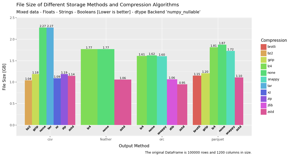

Speed, RAM, size and convenience. Which storage method is best?
Originally appeared here:
Saving Pandas DataFrames Efficiently and Quickly — Parquet vs Feather vs ORC vs CSV


There are periodic proclamations of the coming neuromorphic computing revolution, which uses inspiration from the brain to rethink neural networks and the hardware they run on. While there remain challenges in the field, there have been solid successes and continues to be steady progress in spiking neural network algorithms and neuromorphic hardware. This progress is paving the way for disruption in at least some sectors of artificial intelligence and will reduce the energy consumption per computation at inference and allow artificial intelligence to be pushed further out to the edge. In this article, I will cover some neuromorphic computing and engineering basics, training, the advantages of neuromorphic systems, and the remaining challenges.
The classical use case of neuromorphic systems is for edge devices that need to perform the computation locally and are energy-limited, for example, battery-powered devices. However, one of the recent interests in using neuromorphic systems is to reduce energy usage at data centers, such as the energy needed by large language models (LLMs). For example, OpenAI signed a letter of intent to purchase $51 million of neuromorphic chips from Rain AI in December 2023. This makes sense since OpenAI spends a lot on inference, with one estimate of around $4 billion on running inference in 2024. It also appears that both Intel’s Loihi 2 and IBM’s NorthPole (successor to TrueNorth) neuromorphic systems are designed for use in servers.
The promises of neuromorphic computing can broadly be divided into 1) pragmatic, near-term successes that have already found successes and 2) more aspirational, wacky neuroscientist fever-dream ideas of how spiking dynamics might endow neural networks with something closer to real intelligence. Of course, it’s group 2 that really excites me, but I’m going to focus on group 1 for this post. And there is no more exciting way to start than to dive into terminology.
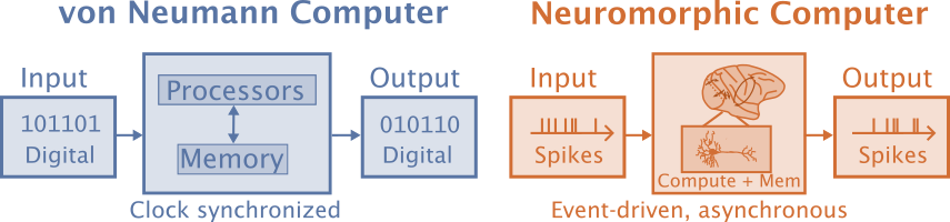
Neuromorphic computation is often defined as computation that is brain-inspired, but that definition leaves a lot to the imagination. Neural networks are more neuromorphic than classical computation, but these days neuromorphic computation is specifically interested in using event-based spiking neural networks (SNNs) for their energy efficiency. Even though SNNs are a type of artificial neural network, the term “artificial neural networks” (ANNs) is reserved for the more standard non-spiking artificial neural networks in the neuromorphic literature. Schuman and colleagues (2022) define neuromorphic computers as non-von Neuman computers where both processing and memory are collocated in artificial neurons and synapses, as opposed to von Neuman computers that separate processing and memory.
Neuromorphic engineering means designing the hardware while “neuromorphic computation” is focused on what is being simulated rather than what it is being simulated on. These are tightly intertwined since the computation is dependent on the properties of the hardware and what is implemented in hardware depends on what is empirically found to work best.
Another related term is NeuroAI, the goal of which is to use AI to gain a mechanistic understanding of the brain and is more interested in biological realism. Neuromorphic computation is interested in neuroscience as a means to an end. It views the brain as a source of ideas that can be used to achieve objectives such as energy efficiency and low latency in neural architectures. A decent amount of the NeuroAI research relies on spike averages rather than spiking neural networks, which allows closer comparison of the majority of modern ANNs that are applied to discrete tasks.
Neuromorphic systems are event-based, which is a paradigm shift from how modern ANN systems work. Even real-time ANN systems typically process one frame at a time, with activity synchronously propagated from one layer to the next. This means that in ANNs, neurons that carry no information require the same processing as neurons that carry critical information. Event-driven is a different paradigm that often starts at the sensor and applies the most work where information needs to be processed. ANNs rely on matrix operations that take the same amount of time and energy regardless of the values in the matrices. Neuromorphic systems use SNNs where the amount of work depends on the number of spikes.
A traditional deployed ANN would often be connected to a camera that synchronously records a frame in a single exposure. The ANN then processes the frame. The results of the frame might then be fed into a tracking algorithm and further processed.
Event-driven systems may start at the sensor with an event camera. Each pixel sends updates asynchronously whenever a change crosses a threshold. So when there is movement in a scene that is otherwise stationary, the pixels that correspond to the movement send events or spikes immediately without waiting for a synchronization signal. The event signals can be sent within tens of microseconds, while a traditional camera might collect at 24 Hz and could introduce a latency that’s in the range of tens of milliseconds. In addition to receiving the information sooner, the information in the event-based system would be sparser and would focus on the movement. The traditional system would have to process the entire scene through each network layer successively.

One of the major challenges of SNNs is training them. Backpropagation algorithms and stochastic gradient descent are the go-to solutions for training ANNs, however, these methods run into difficulty with SNNs. The best way to train SNNs is not yet established and the following methods are some of the more common approaches that are used:
One method of creating SNNs is to bypass training the SNNs directly and instead train ANNs. This approach limits the types of SNNs and hardware that can be used. For example, Sengupta et al. (2019) converted VGG and ResNets to ANNs using an integrate-and-fire (IF) neuron that does not have a leaking or refractory period. They introduce a novel weight-normalization technique to perform the conversion, which involves setting the firing threshold of each neuron based on its pre-synaptic weights. Dr. Priyadarshini Panda goes into more detail in her ESWEEK 2021 SNN Talk.
Advantages:
Disadvantages:
The most common methods currently used to train SNNs are backpropagation-like approaches. Standard backpropagation does not work to train SNNs because 1) the spiking threshold function’s gradient is nonzero except at the threshold where it is undefined and 2) the credit assignment problem needs to be solved in the temporal dimension in addition spatial (or color etc).
In ANNs, the most common activation function is the ReLU. For SNNs, the neuron will fire if the membrane potential is above some threshold, otherwise, it will not fire. This is called a Heaviside function. You could use a sigmoid function instead, but then it would not be a spiking neural network. The solution of using surrogate gradients is to use the standard threshold function in the forward pass, but then use the derivative from a “smoothed” version of the Heaviside function, such as the sigmoid function, in the backward pass (Neftci et al. 2019, Bohte 2011).
Advantages:
Disadvantages:
Spike-timing-dependent plasticity (STDP) is the most well-known form of synaptic plasticity. In most cases, STDP increases the strength of a synapse when a presynaptic (input) spike comes immediately before the postsynaptic spike. Early models have shown promise with STDP on simple unsupervised tasks, although getting it to work well for more complex models and tasks has proven more difficult.
Other biological learning mechanisms include the pruning and creation of both neurons and synapses, homeostatic plasticity, neuromodulators, astrocytes, and evolution. There is even some recent evidence that some primitive types of knowledge can be passed down by epigenetics.
Advantages:
Disadvantages:
Evolutionary optimization is another approach that has some cool applications that works well with small networks. Dr. Catherine Schuman is a leading expert and she gave a fascinating talk on neuromorphic computing to the ICS lab that is available on YouTube.
Advantages:
Disadvantages:
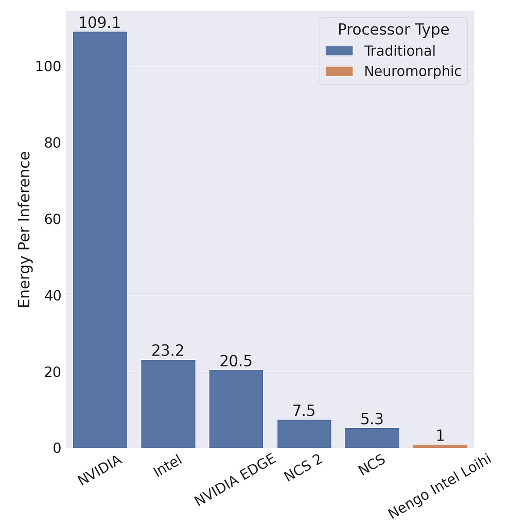
Neuromorphic systems have two main advantages: 1) energy efficiency and 2) low latency. There are a lot of reasons to be excited about the energy efficiency. For example, Intel claimed that their Loihi 2 Neural Processing Unit (NPU) can use 100 times less energy while being as much as 50 times faster than conventional ANNs. Chris Eliasmith compared the energy efficiency of an SNN on neuromorphic hardware with an ANN with the same architecture on standard hardware in a presentation available on YouTube. He found that the SNN is 100 times more energy efficient on Loihi compared to the ANN on a standard NVIDIA GPU and 20 times more efficient than the ANN on an NVIDIA Jetson GPU. It is 5–7 times more energy efficient than the Intel Neural Compute Stick (NCS) and NCS 2. At the same time the SNN achieves a 93.8% accuracy compared to the 92.7% accuracy of the ANN.
Neuromorphic chips are more energy efficient and allow complex deep learning models to be deployed on low-energy edge devices. In October 2024, BrainChip introduced the Akida Pico NPU which uses less than 1 mW of power, and Intel Loihi 2 NPU uses 1 W. That’s a lot less power than NVIDIA Jetson modules that use between 10–50 watts which is often used for embedded ANNs and server GPUs can use around 100 watts.
Comparing the energy efficiency between ANNs and SNNs are difficult because: 1. energy efficiency is dependent on hardware, 2. SNNs and ANNs can use different architectures, and 3. they are suited to different problems. Additionally, the energy used by SNNs scales with the number of spikes and the number of time steps, so the number of spikes and time steps needs to be minimized to achieve the best energy efficiency.
Theoretical analysis is often used to estimate the energy needed by SNNs and ANNs, however, this doesn’t take into account all of the differences between the CPUs and GPUs used for ANNs and the neuromorphic chips for SNNs.
Looking into nature can give us an idea of what might be possible in the future and Mike Davies provided a great anecdote in an Intel Architecture All Access YouTube video:
Consider the capabilities of a tiny cockatiel parrot brain, a two-gram brain running on about 50 mW of power. This brain enables the cockatiel to fly at speeds up to 20 mph, to navigate unknown environments while foraging for food, and even to learn to manipulate objects as tools and utter human words.
In current neural networks, there is a lot of wasted computation. For example, an image encoder takes the same amount of time encoding a blank page as a cluttered page in a “Where’s Waldo?” book. In spiking neural networks, very few units would activate on a blank page and very little computation would be used, while a page containing a lot of features would fire a lot more units and use a lot more computation. In real life, there are often regions in the visual field that contain more features and require more processing than other regions that contain fewer features, like a clear sky. In either case, SNNs only perform work when work needs to be performed, whereas ANNs depend on matrix multiplications that are difficult to use sparsely.
This in itself is exciting. A lot of deep learning currently involves uploading massive amounts of audio or video to the cloud, where the data is processed in massive data centers, spending a lot of energy on the computation and cooling the computational devices, and then the results are returned. With edge computing, you can have more secure and more responsive voice recognition or video recognition, that you can keep on your local device, with orders of magnitude less energy consumption.
When a pixel receptor of an event camera changes by some threshold, it can send an event or spike within microseconds. It doesn’t need to wait for a shutter or synchronization signal to be sent. This benefit is seen throughout the event-based architecture of SNNs. Units can send events immediately, rather than waiting for a synchronization signal. This makes neuromorphic computers much faster, in terms of latency, than ANNs. Hence, neuromorphic processing is better than ANNs for real-time applications that can benefit from low latency. This benefit is reduced if the problem allows for batching and you are measuring speed by throughput since ANNs can take advantage of batching more easily. However, in real-time processing, such as robotics or user interfacing, latency is more important.
One of the challenges is that neuromorphic computing and engineering are progressing at multiple levels at the same time. The details of the models depend on the hardware implementation and empirical results with actualized models guide the development of the hardware. Intel discovered this with their Loihi 1 chips and built more flexibility into their Loihi 2 chips, however, there will always be tradeoffs and there are still many advances to be made on both the hardware and software side.
Hopefully, this will change soon, but commercial hardware isn’t very available. BrainChip’s Akida was the first neuromorphic chip to be commercially available, although apparently, it does not even support the standard leaky-integrate and fire (LIF) neuron. SpiNNaker boards used to be for sale, which was part of the EU Human Brain Project but are no longer available. Intel makes Loihi 2 chips available to some academic researchers via the Intel Neuromorphic Research Community (INRC) program.
The number of neuromorphic datasets is much less than traditional datasets and can be much larger. Some of the common smaller computer vision datasets, such as MNIST (NMNIST, Li et al. 2017) and CIFAR-10 (CIFAR10-DVS, Orchard et al. 2015), have been converted to event streams by displaying the images and recording them using event-based cameras. The images are collected with movement (or “saccades”) to increase the number of spikes for processing. With larger datasets, such as ES-ImageNet (Lin et al. 2021), simulation of event cameras has been used.
The dataset derived from static images might be useful in comparing SNNs with conventional ANNs and might be useful as part of the training or evaluation pipeline, however, SNNs are naturally temporal, and using them for static inputs does not make a lot of sense if you want to take advantage of SNNs temporal properties. Some of the datasets that take advantage of these properties of SNNs include:
Synthetic data can be generated from standard visible camera data without the use of expensive event camera data collections, however these won’t exhibit the high dynamic range and frame rate that event cameras would capture.
Tonic is an example python library that makes it easy to access at least some of these event-based datasets. The datasets themselves can take up a lot more space than traditional datasets. For example, the training images for MNIST is around 10 MB, while in N-MNIST, it is almost 1 GB.
Another thing to take into account is that visualizing the datasets can be difficult. Even the datasets derived from static images can be difficult to match with the original input images. Also, the benefit of using real data is typically to avoid a gap between training and inference, so it would seem that the benefit of using these datasets would depend on their similarity to the cameras used during deployment or testing.

We are in an exciting time with neuromorphic computation, with both the investment in the hardware and the advancements in spiking neural networks. There are still challenges for adoption, but there are proven cases where they are more energy efficient, especially standard server GPUs while having lower latency and similar accuracy as traditional ANNs. A lot of companies, including Intel, IBM, Qualcomm, Analog Devices, Rain AI, and BrainChip have been investing in neuromorphic systems. BrainChip is the first company to make their neuromorphic chips commercially available while both Intel and IBM are on the second generations of their research chips (Loihi 2 and NorthPole respectively). There also seems to have been a particular spike of successful spiking transformers and other deep spiking neural networks in the last couple of years, following the Spikformer paper (Zhou et al. 2022) and the SEW-ResNet paper (Fang et al. 2021).
Originally published at https://neural.vision on November 22, 2024.
Neuromorphic Computing — an Edgier, Greener AI was originally published in Towards Data Science on Medium, where people are continuing the conversation by highlighting and responding to this story.
Originally appeared here:
Neuromorphic Computing — an Edgier, Greener AI
Go Here to Read this Fast! Neuromorphic Computing — an Edgier, Greener AI


Originally appeared here:
Unleash your Salesforce data using the Amazon Q Salesforce Online connector

Originally appeared here:
Reducing hallucinations in large language models with custom intervention using Amazon Bedrock Agents


Originally appeared here:
Deploy Meta Llama 3.1-8B on AWS Inferentia using Amazon EKS and vLLM
Go Here to Read this Fast! Deploy Meta Llama 3.1-8B on AWS Inferentia using Amazon EKS and vLLM


Originally appeared here:
Serving LLMs using vLLM and Amazon EC2 instances with AWS AI chips
Go Here to Read this Fast! Serving LLMs using vLLM and Amazon EC2 instances with AWS AI chips
Understand missing data patterns (MCAR, MNAR, MAR) for better model performance with Missingno
Originally appeared here:
Addressing Missing Data

As generative AI (genAI) models grow in both popularity and scale, so do the computational demands and costs associated with their training and deployment. Optimizing these models is crucial for enhancing their runtime performance and reducing their operational expenses. At the heart of modern genAI systems is the Transformer architecture and its attention mechanism, which is notably compute-intensive.
In a previous post, we demonstrated how using optimized attention kernels can significantly accelerate the performance of Transformer models. In this post, we continue our exploration by addressing the challenge of variable-length input sequences — an inherent property of real-world data, including documents, code, time-series, and more.
In a typical deep learning workload, individual samples are grouped into batches before being copied to the GPU and fed to the AI model. Batching improves computational efficiency and often aids model convergence during training. Usually, batching involves stacking all of the sample tensors along a new dimension — the batch dimension. However, torch.stack requires that all tensors to have the same shape, which is not the case with variable-length sequences.
The traditional way to address this challenge is to pad the input sequences to a fixed length and then perform stacking. This solution requires appropriate masking within the model so that the output is not affected by the irrelevant tensor elements. In the case of attention layers, a padding mask indicates which tokens are padding and should not be attended to (e.g., see PyTorch MultiheadAttention). However, padding can waste considerable GPU resources, increasing costs and slowing development. This is especially true for large-scale AI models.
One way to avoid padding is to concatenate sequences along an existing dimension instead of stacking them along a new dimension. Contrary to torch.stack, torch.cat allows inputs of different shapes. The output of concatenation is single sequence whose length equals the sum of the lengths of the individual sequences. For this solution to work, our single sequence would need to be supplemented by an attention mask that would ensure that each token only attends to other tokens in the same original sequence, in a process sometimes referred to as document masking. Denoting the sum of the lengths of all of the individual by N and adopting ”big O” notation, the size of this mask would need to be O(N²), as would the compute complexity of a standard attention layer, making this solution highly inefficient.
The solution to this problem comes in the form of specialized attention layers. Contrary to the standard attention layer that performs the full set of O(N²) attention scores only to mask out the irrelevant ones, these optimized attention kernels are designed to calculate only the scores that matter. In this post we will explore several solutions, each with their own distinct characteristics. These include:
For teams working with pre-trained models, transitioning to these optimizations might seem challenging. We will demonstrate how HuggingFace’s APIs simplify this process, enabling developers to integrate these techniques with minimal code changes and effort.
Special thanks to Yitzhak Levi and Peleg Nahaliel for their contributions to this post.
To facilitate our discussion we will define a simple generative model (partially inspired by the GPT model defined here). For a more comprehensive guide on building language models, please see one of the many excellent tutorials available online (e.g., here).
We begin by constructing a basic Transformer block, specifically designed to facilitate experimentation with different attention mechanisms and optimizations. While our block performs the same computation as standard Transformer blocks, we make slight modifications to the usual choice of operators in order to support the possibility of PyTorch NestedTensor inputs (as described here).
# general imports
import time, functools

# torch imports
import torch
from torch.utils.data import Dataset, DataLoader
import torch.nn as nn

# Define Transformer settings
BATCH_SIZE = 32
NUM_HEADS = 16
HEAD_DIM = 64
DIM = NUM_HEADS * HEAD_DIM
DEPTH = 24
NUM_TOKENS = 1024
MAX_SEQ_LEN = 1024
PAD_ID = 0
DEVICE = 'cuda'

class MyAttentionBlock(nn.Module):
    def __init__(
            self,
            attn_fn,
            dim,
            num_heads,
            format=None,
            **kwargs
    ):
        super().__init__()
        self.attn_fn = attn_fn
        self.num_heads = num_heads
        self.dim = dim
        self.head_dim = dim // num_heads
        self.norm1 = nn.LayerNorm(dim, bias=False)
        self.norm2 = nn.LayerNorm(dim, bias=False)
        self.qkv = nn.Linear(dim, dim * 3)
        self.proj = nn.Linear(dim, dim)

        # mlp layers
        self.fc1 = nn.Linear(dim, dim * 4)
        self.act = nn.GELU()
        self.fc2 = nn.Linear(dim * 4, dim)

        self.permute = functools.partial(torch.transpose, dim0=1, dim1=2)
        if format == 'bshd':
            self.permute = nn.Identity()

    def mlp(self, x):
        x = self.fc1(x)
        x = self.act(x)
        x = self.fc2(x)
        return x

    def reshape_and_permute(self,x, batch_size):
        x = x.view(batch_size, -1, self.num_heads, self.head_dim)
        return self.permute(x)

    def forward(self, x_in, attn_mask=None):
        batch_size = x_in.size(0)
        x = self.norm1(x_in)
        qkv = self.qkv(x)

        # rather than first reformatting and then splitting the input
        # state, we first split and then reformat q, k, v in order to
        # support PyTorch Nested Tensors
        q, k, v = qkv.chunk(3, -1)
        q = self.reshape_and_permute(q, batch_size)
        k = self.reshape_and_permute(k, batch_size)
        v = self.reshape_and_permute(v, batch_size)

        # call the attn_fn with the input attn_mask
        x = self.attn_fn(q, k, v, attn_mask=attn_mask)

        # reformat output
        x = self.permute(x).reshape(batch_size, -1, self.dim)
        x = self.proj(x)
        x = x + x_in
        x = x + self.mlp(self.norm2(x))
        return x
Building on our programmable Transformer block, we construct a typical Transformer decoder model.
class MyDecoder(nn.Module):
    def __init__(
            self,
            block_fn,
            num_tokens,
            dim,
            num_heads,
            num_layers,
            max_seq_len,
            pad_idx=None
    ):
        super().__init__()
        self.num_heads = num_heads
        self.pad_idx = pad_idx
        self.embedding = nn.Embedding(num_tokens, dim, padding_idx=pad_idx)
        self.positional_embedding = nn.Embedding(max_seq_len, dim)
        self.blocks = nn.ModuleList([
            block_fn(
                dim=dim,
                num_heads=num_heads
            )
            for _ in range(num_layers)])
        self.output = nn.Linear(dim, num_tokens)

    def embed_tokens(self, input_ids, position_ids=None):
        x = self.embedding(input_ids)
        if position_ids is None:
            position_ids = torch.arange(input_ids.shape[1],
                                        device=x.device)
        x = x + self.positional_embedding(position_ids)
        return x

    def forward(self, input_ids, position_ids=None, attn_mask=None):
        # Embed tokens and add positional encoding
        x = self.embed_tokens(input_ids, position_ids)
        if self.pad_idx is not None:
            assert attn_mask is None
            # create a padding mask - we assume boolean masking
            attn_mask = (input_ids != self.pad_idx)
            attn_mask = attn_mask.view(BATCH_SIZE, 1, 1, -1)
                .expand(-1, self.num_heads, -1, -1)

        for b in self.blocks:
            x = b(x, attn_mask)

        logits = self.output(x)
        return logits
Next, we create a dataset containing sequences of variable lengths, where each sequence is made up of randomly generated tokens. For simplicity, we (arbitrarily) select a fixed distribution for the sequence lengths. In real-world scenarios, the distribution of sequence lengths typically reflects the nature of the data, such as the length of documents or audio segments. Note, that the distribution of lengths directly affects the computational inefficiencies caused by padding.
# Use random data
class FakeDataset(Dataset):
    def __len__(self):
        return 1000000

    def __getitem__(self, index):
        length = torch.randint(1, MAX_SEQ_LEN, (1,))
        sequence = torch.randint(1, NUM_TOKENS, (length + 1,))
        input = sequence[:-1]
        target = sequence[1:]
        return input, target

def pad_sequence(sequence, length, pad_val):
    return torch.nn.functional.pad(
        sequence,
        (0, length - sequence.shape[0]),
        value=pad_val
    )

def collate_with_padding(batch):
    padded_inputs = []
    padded_targets = []
    for b in batch:
        padded_inputs.append(pad_sequence(b[0], MAX_SEQ_LEN, PAD_ID))
        padded_targets.append(pad_sequence(b[1], MAX_SEQ_LEN, PAD_ID))
    padded_inputs = torch.stack(padded_inputs, dim=0)
    padded_targets = torch.stack(padded_targets, dim=0)
    return {
        'inputs': padded_inputs,
        'targets': padded_targets
    }

def data_to_device(data, device):
    if isinstance(data, dict):
        return {
            key: data_to_device(val,device)
            for key, val in data.items()
        }
    elif isinstance(data, (list, tuple)):
        return type(data)(
            data_to_device(val, device) for val in data
        )
    elif isinstance(data, torch.Tensor):
        return data.to(device=device, non_blocking=True)
    else:
        return data.to(device=device)
Lastly, we implement a main function that performs training/evaluation on input sequences of varying length.
def main(
    block_fn,
    data_collate_fn=collate_with_padding,
    pad_idx=None,
    train=True,
    compile=False
):
    torch.random.manual_seed(0)
    device = torch.device(DEVICE)
    torch.set_float32_matmul_precision("high")

    # Create dataset and dataloader
    data_set = FakeDataset()
    data_loader = DataLoader(
        data_set,
        batch_size=BATCH_SIZE,
        collate_fn=data_collate_fn,
        num_workers=12,
        pin_memory=True,
        drop_last=True
    )

    model = MyDecoder(
        block_fn=block_fn,
        num_tokens=NUM_TOKENS,
        dim=DIM,
        num_heads=NUM_HEADS,
        num_layers=DEPTH,
        max_seq_len=MAX_SEQ_LEN,
        pad_idx=pad_idx
    ).to(device)

    if compile:
        model = torch.compile(model)

    # Define loss and optimizer
    criterion = torch.nn.CrossEntropyLoss(ignore_index=PAD_ID)
    optimizer = torch.optim.SGD(model.parameters())

    def train_step(model, inputs, targets,
                   position_ids=None, attn_mask=None):
        with torch.amp.autocast(DEVICE, dtype=torch.bfloat16):
            outputs = model(inputs, position_ids, attn_mask)
            outputs = outputs.view(-1, NUM_TOKENS)
            targets = targets.flatten()
            loss = criterion(outputs, targets)
        optimizer.zero_grad(set_to_none=True)
        loss.backward()
        optimizer.step()

    @torch.no_grad()
    def eval_step(model, inputs, targets,
                  position_ids=None, attn_mask=None):
        with torch.amp.autocast(DEVICE, dtype=torch.bfloat16):
            outputs = model(inputs, position_ids, attn_mask)
            if outputs.is_nested:
                outputs = outputs.data._values
                targets = targets.data._values
            else:
                outputs = outputs.view(-1, NUM_TOKENS)
                targets = targets.flatten()
            loss = criterion(outputs, targets)
        return loss

    if train:
        model.train()
        step_fn = train_step
    else:
        model.eval()
        step_fn = eval_step

    t0 = time.perf_counter()
    summ = 0
    count = 0

    for step, data in enumerate(data_loader):
        # Copy data to GPU
        data = data_to_device(data, device=device)
        step_fn(model, data['inputs'], data['targets'],
                       position_ids=data.get('indices'),
                       attn_mask=data.get('attn_mask'))

        # Capture step time
        batch_time = time.perf_counter() - t0
        if step > 20:  # Skip first steps
            summ += batch_time
            count += 1
        t0 = time.perf_counter()
        if step >= 100:
            break
    print(f'average step time: {summ / count}')
For our baseline experiments, we configure our Transformer block to utilize PyTorch’s SDPA mechanism. In our experiments, we run both training and evaluation, both with and without torch.compile. These were run on an NVIDIA H100 with CUDA 12.4 and PyTorch 2.5.1
from torch.nn.functional import scaled_dot_product_attention as sdpa
block_fn = functools.partial(MyAttentionBlock, attn_fn=sdpa)
causal_block_fn = functools.partial(
    MyAttentionBlock,
    attn_fn=functools.partial(sdpa, is_causal=True)
)

for mode in ['eval', 'train']:
    for compile in [False, True]:
        block_func = causal_block_fn
            if mode == 'train' else block_fn
        print(f'{mode} with {collate}, '
              f'{"compiled" if compile else "uncompiled"}')
        main(block_fn=block_func,
             pad_idx=PAD_ID,
             train=mode=='train',
             compile=compile)
Performance Results:
In this section, we will explore several optimization techniques for handling variable-length input sequences in Transformer models.
Our first optimization relates not to the attention kernel but to our padding mechanism. Rather than padding the sequences in each batch to a constant length, we pad to the length of the longest sequence in the batch. The following block of code consists of our revised collation function and updated experiments.
def collate_pad_to_longest(batch):
    padded_inputs = []
    padded_targets = []
    max_length = max([b[0].shape[0] for b in batch])
    for b in batch:
        padded_inputs.append(pad_sequence(b[0], max_length, PAD_ID))
        padded_targets.append(pad_sequence(b[1], max_length, PAD_ID))
    padded_inputs = torch.stack(padded_inputs, dim=0)
    padded_targets = torch.stack(padded_targets, dim=0)
    return {
        'inputs': padded_inputs,
        'targets': padded_targets
    }

for mode in ['eval', 'train']:
    for compile in [False, True]:
        block_func = causal_block_fn
            if mode == 'train' else block_fn
        print(f'{mode} with {collate}, '
              f'{"compiled" if compile else "uncompiled"}')
        main(block_fn=block_func,
             data_collate_fn=collate_pad_to_longest,
             pad_idx=PAD_ID,
             train=mode=='train',
             compile=compile)
Padding to the longest sequence in each batch results in a slight performance acceleration:
Next, we take advantage of the built-in support for PyTorch NestedTensors in SDPA in evaluation mode. Currently a prototype feature, PyTorch NestedTensors allows for grouping together tensors of varying length. These are sometimes referred to as jagged or ragged tensors. In the code block below, we define a collation function for grouping our sequences into NestedTensors. We also define an indices entry so that we can properly calculate the positional embeddings.
PyTorch NestedTensors are supported by a limited number of PyTorch ops. Working around these limitations can require some creativity. For example, addition between NestedTensors is only supported when they share precisely the same “jagged” shape. In the code below we use a workaround to ensure that the indices entry shares the same shape as the model inputs.
def nested_tensor_collate(batch):
    inputs = torch.nested.as_nested_tensor([b[0] for b in batch],
                                           layout=torch.jagged)
    targets = torch.nested.as_nested_tensor([b[1] for b in batch],
                                            layout=torch.jagged)
    indices = torch.concat([torch.arange(b[0].shape[0]) for b in batch])

    # workaround for creating a NestedTensor with identical "jagged" shape
    xx = torch.empty_like(inputs)
    xx.data._values[:] = indices

    return {
        'inputs': inputs,
        'targets': targets,
        'indices': xx
    }

for compile in [False, True]:
    print(f'eval with nested tensors, '
          f'{"compiled" if compile else "uncompiled"}')
    main(
        block_fn=block_fn,
        data_collate_fn=nested_tensor_collate,
        train=False,
        compile=compile
    )
Although, with torch.compile, the NestedTensor optimization results in a step time of 131 ms, similar to our baseline result, in compiled mode the step time drops to 42 ms for an impressive ~3x improvement.
In our previous post we demonstrated the use of FlashAttention and its impact on the performance of a transformer model. In this post we demonstrate the use of flash_attn_varlen_func from flash-attn (2.7.0), an API designed for use with variable-sized inputs. To use this function, we concatenate all of the sequences in the batch into a single sequence. We also create a cu_seqlens tensor that points to the indices within the concatenated tensor where each of the individual sequences start. The code block below includes our collation function followed by evaluation and training experiments. Note, that flash_attn_varlen_func does not support torch.compile (at the time of this writing).
def collate_concat(batch):
    inputs = torch.concat([b[0] for b in batch]).unsqueeze(0)
    targets = torch.concat([b[1] for b in batch]).unsqueeze(0)
    indices = torch.concat([torch.arange(b[0].shape[0]) for b in batch])
    seqlens = torch.tensor([b[0].shape[0] for b in batch])
    seqlens = torch.cumsum(seqlens, dim=0, dtype=torch.int32)
    cu_seqlens = torch.nn.functional.pad(seqlens, (1, 0))

    return {
        'inputs': inputs,
        'targets': targets,
        'indices': indices,
        'attn_mask': cu_seqlens
    }

from flash_attn import flash_attn_varlen_func
fa_varlen = lambda q, k, v, attn_mask: flash_attn_varlen_func(
    q.squeeze(0),
    k.squeeze(0),
    v.squeeze(0),
    cu_seqlens_q=attn_mask,
    cu_seqlens_k=attn_mask,
    max_seqlen_q=MAX_SEQ_LEN,
    max_seqlen_k=MAX_SEQ_LEN
).unsqueeze(0)

fa_varlen_causal = lambda q, k, v, attn_mask: flash_attn_varlen_func(
    q.squeeze(0),
    k.squeeze(0),
    v.squeeze(0),
    cu_seqlens_q=attn_mask,
    cu_seqlens_k=attn_mask,
    max_seqlen_q=MAX_SEQ_LEN,
    max_seqlen_k=MAX_SEQ_LEN,
    causal=True
).unsqueeze(0)

block_fn = functools.partial(MyAttentionBlock,
                             attn_fn=fa_varlen,
                             format='bshd')

causal_block_fn = functools.partial(MyAttentionBlock,
                                    attn_fn=fa_varlen_causal,
                                    format='bshd')

print('flash-attn eval')
main(
    block_fn=block_fn,
    data_collate_fn=collate_concat,
    train=False
)

print('flash-attn train')
main(
    block_fn=causal_block_fn,
    data_collate_fn=collate_concat,
    train=True,
)
The impact of this optimization is dramatic, 51 ms for evaluation and 160 ms for training, amounting to 2.6x and 2.1x performance boosts compared to our baseline experiment.
In our previous post we demonstrated the use of the memory_efficient_attention operator from xFormers (0.0.28). Here we demonstrate the use of BlockDiagonalMask, specifically designed for input sequences of arbitrary length. The required collation function appears in the code block below followed by the evaluation and training experiments. Note, that torch.compile failed in training mode.
from xformers.ops import fmha
from xformers.ops import memory_efficient_attention as mea

def collate_xformer(batch):
    inputs = torch.concat([b[0] for b in batch]).unsqueeze(0)
    targets = torch.concat([b[1] for b in batch]).unsqueeze(0)
    indices = torch.concat([torch.arange(b[0].shape[0]) for b in batch])
    seqlens = [b[0].shape[0] for b in batch]
    batch_sizes = [1 for b in batch]
    block_diag = fmha.BlockDiagonalMask.from_seqlens(seqlens, device='cpu')
    block_diag._batch_sizes = batch_sizes

    return {
        'inputs': inputs,
        'targets': targets,
        'indices': indices,
        'attn_mask': block_diag
    }

mea_eval = lambda q, k, v, attn_mask: mea(
    q,k,v, attn_bias=attn_mask)

mea_train = lambda q, k, v, attn_mask: mea(
    q,k,v, attn_bias=attn_mask.make_causal())

block_fn = functools.partial(MyAttentionBlock,
                             attn_fn=mea_eval,
                             format='bshd')

causal_block_fn = functools.partial(MyAttentionBlock,
                             attn_fn=mea_train,
                             format='bshd')

print(f'xFormer Attention ')
for compile in [False, True]:
    print(f'eval with xFormer Attention, '
          f'{"compiled" if compile else "uncompiled"}')
    main(block_fn=block_fn,
         train=False,
         data_collate_fn=collate_xformer,
         compile=compile)

print(f'train with xFormer Attention')
main(block_fn=causal_block_fn,
     train=True,
     data_collate_fn=collate_xformer)
The resultant step time were 50 ms and 159 ms for evaluation and training without torch.compile. Evaluation with torch.compile resulted in a step time of 42 ms.
The table below summarizes the results of our optimization methods.

The best performer for our toy model is xFormer’s memory_efficient_attention which delivered a ~3x performance for evaluation and ~2x performance for training. We caution against deriving any conclusions from these results as the performance impact of different attention functions can vary significantly depending on the specific model and use case.
The tools and techniques described above are easy to implement when creating a model from scratch. However, these days it is not uncommon for ML developers to adopt existing (pretrained) models and finetune them for their use case. While the optimizations we have described can be integrated without changing the set of model weights and without altering the model behavior, it is not entirely clear what the best way to do this is. In an ideal world, our ML framework would allow us to program the use of an attention mechanism that is optimized for variable-length inputs. In this section we demonstrate how to optimize HuggingFace models for variable-length inputs.
To facilitate the discussion, we create a toy example in which we train a HuggingFace GPT2LMHead model on variable-length sequences. This requires adapting our random dataset and data-padding collation function according to HuggingFace’s input specifications.
from transformers import GPT2Config, GPT2LMHeadModel

# Use random data
class HuggingFaceFakeDataset(Dataset):
    def __len__(self):
        return 1000000

    def __getitem__(self, index):
        length = torch.randint(1, MAX_SEQ_LEN, (1,))
        input_ids = torch.randint(1, NUM_TOKENS, (length,))
        labels = input_ids.clone()
        labels[0] = PAD_ID # ignore first token
        return {
            'input_ids': input_ids,
            'labels': labels
        }
        return input_ids, labels

def hf_collate_with_padding(batch):
    padded_inputs = []
    padded_labels = []
    for b in batch:
        input_ids = b['input_ids']
        labels = b['labels']
        padded_inputs.append(pad_sequence(input_ids, MAX_SEQ_LEN, PAD_ID))
        padded_labels.append(pad_sequence(labels, MAX_SEQ_LEN, PAD_ID))
    padded_inputs = torch.stack(padded_inputs, dim=0)
    padded_labels = torch.stack(padded_labels, dim=0)
    return {
        'input_ids': padded_inputs,
        'labels': padded_labels,
        'attention_mask': (padded_inputs != PAD_ID)
    }
Our training function instantiates a GPT2LMHeadModel based on the requested GPT2Config and proceeds to train it on our variable-length sequences.
def hf_main(
    config,
    collate_fn=hf_collate_with_padding,
    compile=False
):
    torch.random.manual_seed(0)
    device = torch.device(DEVICE)
    torch.set_float32_matmul_precision("high")

    # Create dataset and dataloader
    data_set = HuggingFaceFakeDataset()
    data_loader = DataLoader(
        data_set,
        batch_size=BATCH_SIZE,
        collate_fn=collate_fn,
        num_workers=12 if DEVICE == "CUDA" else 0,
        pin_memory=True,
        drop_last=True
    )

    model = GPT2LMHeadModel(config).to(device)

    if compile:
        model = torch.compile(model)

    # Define loss and optimizer
    criterion = torch.nn.CrossEntropyLoss(ignore_index=PAD_ID)
    optimizer = torch.optim.SGD(model.parameters())

    model.train()

    t0 = time.perf_counter()
    summ = 0
    count = 0

    for step, data in enumerate(data_loader):
        # Copy data to GPU
        data = data_to_device(data, device=device)
        input_ids = data['input_ids']
        labels = data['labels']
        position_ids = data.get('position_ids')
        attn_mask = data.get('attention_mask')
        with torch.amp.autocast(DEVICE, dtype=torch.bfloat16):
            outputs = model(input_ids=input_ids,
                            position_ids=position_ids,
                            attention_mask=attn_mask)
            logits = outputs.logits[..., :-1, :].contiguous()
            labels = labels[..., 1:].contiguous()
            loss = criterion(logits.view(-1, NUM_TOKENS), labels.flatten())

        optimizer.zero_grad(set_to_none=True)
        loss.backward()
        optimizer.step()

        # Capture step time
        batch_time = time.perf_counter() - t0
        if step > 20:  # Skip first steps
            summ += batch_time
            count += 1
        t0 = time.perf_counter()
        if step >= 100:
            break
    print(f'average step time: {summ / count}')
In the callback below we call our training function with the default sequence-padding collator.
config = GPT2Config(
        n_layer=DEPTH,
        n_embd=DIM,
        n_head=NUM_HEADS,
        vocab_size=NUM_TOKENS,
    )

for compile in [False, True]:
    print(f"HF GPT2 train with SDPA, compile={compile}")
    hf_main(config=config, compile=compile)
The resultant step times are 815 ms without torch.compile and 440 ms with torch.compile.
We now take advantage of HuggingFace’s built-in support for FlashAttention2, by setting the attn_implementation parameter to “flash_attention_2”. Behind the scenes, HuggingFace will unpad the padded data input and then pass them to the optimized flash_attn_varlen_func function we saw above:
flash_config = GPT2Config(
        n_layer=DEPTH,
        n_embd=DIM,
        n_head=NUM_HEADS,
        vocab_size=NUM_TOKENS,
        attn_implementation='flash_attention_2'
    )

print(f"HF GPT2 train with flash")
hf_main(config=flash_config)
The resultant time step is 620 ms, amounting to a 30% boost (in uncompiled mode) with just a simple flick of a switch.
Of course, padding the sequences in the collation function only to have them unpadded, hardly seems sensible. In a recent update to HuggingFace, support was added for passing in concatenated (unpadded) sequences to a select number of models. Unfortunately, (as of the time of this writing) our GPT2 model did not make the cut. However, adding support requires just five small line additions changes to modeling_gpt2.py in order to propagate the sequence position_ids to the flash-attention kernel. The full patch appears in the block below:
@@ -370,0 +371 @@
+        position_ids = None
@@ -444,0 +446 @@
+            position_ids=position_ids
@@ -611,0 +614 @@
+        position_ids=None
@@ -621,0 +625 @@
+            position_ids=position_ids
@@ -1140,0 +1145 @@
+                    position_ids=position_ids
We define a collate function that concatenates our sequences and train our hugging face model on unpadded sequences. (Also see the built-in DataCollatorWithFlattening utility.)
def collate_flatten(batch):
    input_ids = torch.concat([b['input_ids'] for b in batch]).unsqueeze(0)
    labels = torch.concat([b['labels'] for b in batch]).unsqueeze(0)
    position_ids = [torch.arange(b['input_ids'].shape[0]) for b in batch]
    position_ids = torch.concat(position_ids)

    return {
        'input_ids': input_ids,
        'labels': labels,
        'position_ids': position_ids
    }

print(f"HF GPT2 train with flash, no padding")
hf_main(config=flash_config, collate_fn=collate_flatten)
The resulting step time is 323 ms, 90% faster than running flash-attention on the padded input.
The results of our HuggingFace experiments are summarized below.
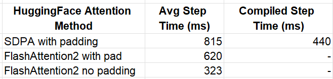
With little effort, we were able to boost our runtime performance by 2.5x when compared to the uncompiled baseline experiment, and by 36% when compared to the compiled version.
In this section, we demonstrated how the HuggingFace APIs allow us to leverage the optimized kernels in FlashAttention2, significantly boosting the training performance of existing models on sequences of varying length.
As AI models continue to grow in both popularity and complexity, optimizing their performance has become essential for reducing runtime and costs. This is especially true for compute-intensive components like attention layers. In this post, we have continued our exploration of attention layer optimization, and demonstrated new tools and techniques for enhancing Transformer model performance. For more insights on AI model optimization, be sure to check out the first post in this series as well as our many other posts on this topic.
Optimizing Transformer Models for Variable-Length Input Sequences was originally published in Towards Data Science on Medium, where people are continuing the conversation by highlighting and responding to this story.
Originally appeared here:
Optimizing Transformer Models for Variable-Length Input Sequences
Go Here to Read this Fast! Optimizing Transformer Models for Variable-Length Input Sequences