Simple Random Sampling (SRS) works, but if you do not know Probability Proportional to Size Sampling (PPS), you are risking yourself some critical statistical mistakes. Learn why, when, and how you can use PPS Sampling here!
Rahul decides to measure the “pulse” of customers buying from his online store. He wanted to know how they are feeling, what is going well, and what can be improved for user experience. Because he has learnt about mathematics and he knows the numbers game, he decides to have a survey with 200 of his 2500 customers. Rahul uses Simple Random Sampling and gets 200 unique customer IDs. He sends them an online survey, and receives the results. According to the survey, the biggest impediment with the customers was lack of payment options while checking out. Rahul contacts a few vendors, and invests in rolling out a few more payment options. Unfortunately, the results after six months showed that there was no significant increase in the revenue. His analysis fails, and he wonders if the resources were spent in the right place.
Rahul ignored the biggest truth of all. All the customers are not homogenous. Some spend more, some spend less, and some spend a lot. Don’t be like Rahul. Be like Sheila, and learn how you can use PPS Sampling — an approach that ensures that your most important (profitable) customers never get overlooked — for reasonable and robust statistical analysis.
What is Sampling?
Before I discuss PPS Sampling, I will briefly mention what sampling is. Sampling is a statistical technique which allows us to take a portion of our population, and use this portion of our population to measure some characteristics of the population. For example, taking a sample of blood to measure if we have an infectious disease, taking a sample of rice pudding to check if sugar is enough, and taking a sample of customers to measure the general pulse of customers. Because we cannot afford measuring each and every single unit of the entire population, it is best to take a sample and then infer the population characteristics. This suffices for a definition here. If you need more information about sampling, the Internet has a lot of resources.
What is PPS Sampling?
Probability Proportional to Size (PPS) Sampling is a sampling technique, where the probability of selection of a unit in the sample is dependent upon the size of a defined variable or an auxiliary variable.
WHAT???
Let me explain with the help of an example. Suppose you have an online store, and there are 1000 people who are your customers. Some customers spend a lot of money and bring a lot of revenue to your organization. These are very important customers. You need to ensure that your organization serve the interests of these customers in the best way possible.
If you want to understand the mood of these customers, you would prefer a situation where your sample has a higher representation of these customers. This is exactly what PPS allows you to do. If you use PPS Sampling, the probability of selecting the highest revenue generating customers is also high. This makes sense. The revenue in this case is the auxiliary or dependency variable.
PPS Sampling vs SRS Sampling
Simple Random Sampling is great. No denial of that fact, but it’s not the only tool that you have in your arsenal. SRS works best for the situations where your population is homogenous. Unfortunately for many practical business applications, the audience or population is not homogenous. If you do an analysis with wrong assumption, you will get the wrong inferences. SRS Sampling gives the same probability of selection to each unit of the population which is different from PPS Sampling.
Why should I use PPS Sampling?
As the title of this article says, you cannot afford not knowing PPS Sampling. Here are five reasons why.
Better Representativeness — By prioritizing the units that have a higher impact on your variable of interest (revenue), you are ensuring that the sample has a better representativeness. This contrasts with SRS which assumes that a customer spending 100 USD a month is equal to the customer spending 1000 USD a month. Nein, no, nahin, that is not the case.
Focus on High-Impact Units — According to the Pareto principle, 80% of your revenue is generated by 20% of the customers. You need to ensure you do not mess up with these 20% of the customers. By ensuring a sample having a higher say for these 20% customers, you will avoid yourself and them any unseen surprises.
Resource Efficiency — There is a thumb’s rule in statistics which says that on an average if you have a sample of 30, you can get close to the estimated population parameters. Note that this is only a thumb rule. PPS Sampling allows you to use the resources you have in designing, distributing, and analyzing interventions are used judiciously.
Improved Accuracy — Because we are putting more weight on the units that have a larger impact on our variable of interest, we are more accurate with our analysis. This may not be possible with just SRS. The sample estimates which you get from PPS Sampling are weighted for the units that have a higher impact. In simple words, you are working for those who pay the most.
Better Decision-Making — When you use PPS sampling, you’re making decisions based on data that actually matters. If you only sample customers randomly, you might end up with feedback or insights from people whose opinions have little influence on your revenue. With PPS, you’re zeroing in on the important customers. It’s like asking the right people the right questions instead of just anyone in the crowd.
PPS Implementation in Python
Slightly more than six years ago, I wrote this article on Medium which is one of my most-read articles, and is shown on the first page when you search for Probability Proportional to Size Sampling (PPS Sampling, from now onwards). The article shows how one can use PPS Sampling for representative sampling using Python. A lot of water has flown under the bridge since then, and I now I have much more experience in causal inference, and my Python skills have improved considerably too. The code linked above used systematic PPS Sampling, whereas the new code uses random PPS Sampling.
Here is the new code that can do the same in a more efficient way.
import numpy as np import pandas as pd
# Simulate customer data np.random.seed(42) # For reproducibility num_customers = 1000 customers = [f"C{i}" for i in range(1, num_customers + 1)]
# Simulate revenue data (e.g., revenue between $100 and $10,000) revenues = np.random.randint(100, 10001, size=num_customers)
# Perform PPS Sampling sample_size = 60 # decide for your analysis
# the actual PPS algorithm sample_indices = np.random.choice( customer_data.index, size=sample_size, replace=False, # No replacement, we are not replacing the units p=customer_data["Selection_Prob"] )
I am sure if you have read until here, you may be wondering that how is it possible that there will be no cons of PPS Sampling. Well, it has some. Here are they.
PPS Sampling is complex to understand so it may not always have a buy-in from the management of an organization. In that case, it is the data scientist’s job to ensure that the benefits are explained in the right manner.
PPS Sampling requires that there is a dependency variable. For example, in our case we chose revenue as a variable upon which we select our units. If you are in agriculture industry, this could be the land size for measuring yield of a cropping season.
PPS Sampling is perceived to be biased against the units having a lower impact. Well, it is not biased and the smaller units also have a chance of getting selected, but the probability is lower for them.
Conclusion
In this article, I explained to you what PPS Sampling is, why it’s better and more resource-efficient than SRS Sampling, and how you can implement it using Python. I am curious to hear more examples from your work to see how you implement PPS at your work.
Welcome to the penultimate monthly recap of 2024 — could we really be this close to the end of the year?! We’re sure that you, like us, are hard at work tying up loose ends and making a final push on your various projects. We have quite a few of those on our end, and one exciting update we’re thrilled to share with our community already is that TDS is now active on Bluesky. If you’re one of the many recent arrivals to the platform (or have been thinking about taking the plunge), we encourage you to follow our account.
What else is on our mind? All the fantastic articles our authors have published in recent weeks, inspiring our readers to learn new skills and explore emerging topics in data science and AI. Our monthly highlights cover a lot of ground—as they usually do—and provide multiple accessible entryways into timely technical topics, from knowledge graphs to RAG evaluation. Let’s dive in.
Monthly Highlights
Agentic Mesh: The Future of Generative AI-Enabled Autonomous Agent Ecosystems What will it take for autonomous agents to find each other, collaborate, interact, and transact in a safe, efficient, and trusted fashion? Eric Broda presents his exciting vision for the agentic mesh, a framework that will act as the seamless connecting tissue for AI agents.
Why ETL-Zero? Understanding the shift in Data Integration “Instead of requiring the explicit extraction, transformation and loading of data in separate steps, as is traditionally the case, data should flow seamlessly between different systems.” Sarah Lea introduces a novel approach for creating a simplified ETL process with Python.
Economics of Hosting Open Source LLMs As LLM usage has skyrocketed in the past year or so, practitioners have increasingly asked themselves what the most efficient way to deploy these models might be. Ida Silfverskiöld offers a detailed breakdown of the various factors to consider and how different providers stack up when it comes to processing time, cold start delays, and CPU, memory, and GPU costs.
How to Reduce Python Runtime for Demanding Tasks Everyone wants their code to run faster, but hitting a plateau is all but inevitable when dealing with particularly heavy workloads. Still, as Jiayan Yin shows in her highly actionable post, there might still be GPU optimization options you haven’t taken advantage of to speed up your Python code.
How to Create a RAG Evaluation Dataset From Documents As Dr. Leon Eversberg explains in his recent tutorial, “by uploading PDF files and storing them in a vector database, we can retrieve this knowledge via a vector similarity search and then insert the retrieved text into the LLM prompt as additional context.” The result? A robust approach for evaluating RAG workflows and a reduced chance for hallucinations.
Thank you for supporting the work of our authors! We love publishing articles from new authors, so if you’ve recently written an interesting project walkthrough, tutorial, or theoretical reflection on any of our core topics, don’t hesitate to share it with us.
Do dogs poop facing North and South? Turns out they do! Want to learn how to measure this at home using a compass app, Bayesian statistics, and one dog (dog not included)? Jump in!
Introduction
This is my dog. His name is Auri and he is a 5 year old Cavalier King Charles Spaniel.
Auri (image by author)
As many other dog owners, during our walks I noticed that Auri has a very particular ritual when he needs to go to the bathroom. When he finds a perfect spot he starts circling around something like a compass.
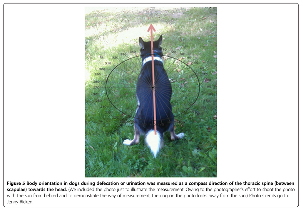
At first I was simply amused by this behaviour. After all, who knows what goes through a dog’s mind? But after a while I remembered reading a research paper from 2013 titled “Dogs are sensitive to small variations of the Earth’s magnetic field”. The research was conducted on a relatively large sample of dogs and confirmed that “dogs preferred to excrete with the body being aligned along the north-south axis”.
Now that could be an interesting research to try out! I thought to myself. And how lucky that I have a perfect test subject, a lovely canine of my own. I decided to replicate the findings and confirm (or debunk!) the hypothesis with Auri, my N=1 unsuspecting research participant.
And so began my long journey of data collection spanning multiple months and capturing over 150 of “alignment sessions” if you catch my drift.
Data Collection
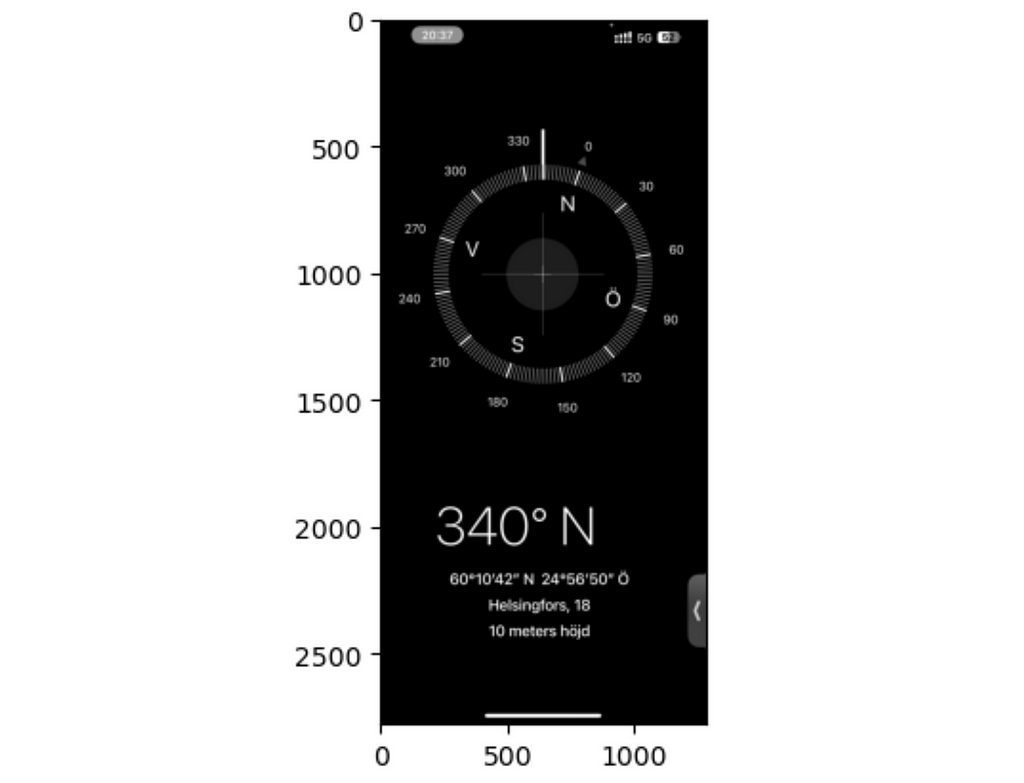
For my study, I needed to have a compass measurement for every time Auri pooped. Thank to modern technological advancements we not only have a calculator app for iPad but also a fairly accurate compass on a phone. And that’s what I decided to use.
The approach was very simple. Every time my dog settled to have some private time I opened the compass app, aligned my phone along Auri’s body and took a screenshot. In the original paper the authors eloquently called the alignment as a compass direction of the thoracic spine (between scapulae) towards the head. Very scientific. All it means is that the compass arrow is supposed to point at the same direction as dog’s head.
Anyways, that’s what I did in total 150 something times over the course of a few months. I could almost sense the passer bys’ confusion mixed with curiosity as I was seemingly taking pictures of all my dog’s relief acts. But was it worth it? Let’s find out!
Analysis
I’ll briefly discuss the data extraction and preprocessing here and then jump straight to working with circular distributions and hypothesis testing.
As always, all the code can be found on my GitHub here: Data Wondering.
How to process app screenshots?
After data collection I had a series of screenshots of the compass app:
Compass app screenshot (image by author)
Being lazy as I am I didn’t feel like scrolling through all of them patiently writing down the compass degrees. So I decided to send all those images to my notebook and automate the process.
The task was simple — all I needed from the images was the big numbers at the bottom of the screen. Fortunately, there are a lot of small pretrained networks out there that can do basic OCR (stands for Optical character recognition). I opted for an easyocr package which was a bit on a slower end but free and easy to work with.
I’ll walk you through a quick example of using easyocr alongside with opencv to extract the numbers from a single screenshot.
Finally, I use easyocr to extract the numbers from the image. It does extract both the number and the confidence score but I am only interested in the number.
import easyocr

reader = easyocr.Reader(['en'])
result = reader.readtext(gray[1850:2100, 200:580])
for bbox, text, prob in result:
    print(f"Detected text: {text} with confidence {prob}")
>> Detected text: 340 with confidence 0.999995182215476
And that’s it! I wrote a simple for loop to iterate through all the screenshots and saved the results to a CSV file.
I don’t usually work with circular distributions so I had to do some reading. Unlike regular data that we are used to, circular data has a peculiar property: the “ends” of the distribution are connected.
For example, if you take the distribution of hours in a day, you would find that the distance between 23:00 and 00:00 is the same as between 00:00 and 01:00. Or, in the case of compass degrees, the distance between 359° and 0° is the same as between 0° and 1°.
Even calculating a sample mean is not straightforward. A standard arithmetic mean between 360° and 0° would give 180° although both 360° and 0° point to the exact same direction.
Similarly in my case, I got almost perfectly opposite estimates when calculating the mean in an arithmetic and in correct way. I converted the degrees to radians using a helper function from this nice library: pingouin and calculated the mean using the circ_mean function.
Next, I wanted to visualize the compass distribution. I used the Von Mises distribution to model the circular data and drew the polar plot using matplotlib.
The Von Mises distribution is the circular analogue of the normal distribution. It is defined by two parameters: the mean location μ and the concentration κ. The concentration parameter controls the spread and is analogous to the inverse of the variance. When κ is 0 the distribution is uniform, as κ increases the distribution contracts around the mean.
Let’s import the necessary libraries and define the helper functions:
import pandas as pd import numpy as np import matplotlib.pyplot as plt import seaborn as sns
from scipy.stats import vonmises from pingouin import convert_angles from typing import Tuple, List
def vonmises_kde(series: np.ndarray, kappa: float, n_bins: int = 100) -> Tuple[np.ndarray, np.ndarray]: """ Estimate a von Mises kernel density estimate (KDE) over circular data using scipy.
Parameters: series: np.ndarray The input data in radians, expected to be a 1D array. kappa: float The concentration parameter for the von Mises distribution. n_bins: int The number of bins for the KDE estimate (default is 100).
Returns: bins: np.ndarray The bin edges (x-values) used for the KDE. kde: np.ndarray The estimated density values (y-values) for each bin. """ bins = np.linspace(-np.pi, np.pi, n_bins) kde = np.zeros(n_bins)
for angle in series: kde += vonmises.pdf(bins, kappa, loc=angle)
kde = kde / len(series) return bins, kde
def plot_circular_distribution( data: pd.DataFrame, plot_type: str = 'kde', bins: int = 30, figsize: tuple = (4, 4), **kwargs ) -> None: """ Plot a compass rose with either KDE or histogram for circular data.
Parameters: ----------- data: pd.DataFrame DataFrame containing 'degrees'and 'radians' columns with circular data plot_type: str Type of plot to create: 'kde' or 'histogram' bins: int Number of bins for histogram or smoothing parameter for KDE figsize: tuple Figure size as (width, height) **kwargs: dict Additional styling arguments for histogram (color, edgecolor, etc.) """ plt.figure(figsize=figsize) ax = plt.subplot(111, projection='polar')
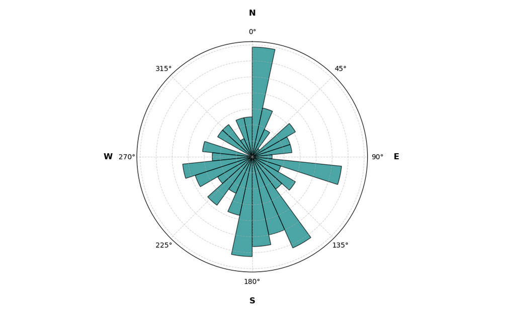
Circular histogram of doggy business (image by author)
From the histogram it’s clear that Auri has his preferences when choosing the relief direction. There’s a clear spike towards the North and a dip towards the South. Nice!
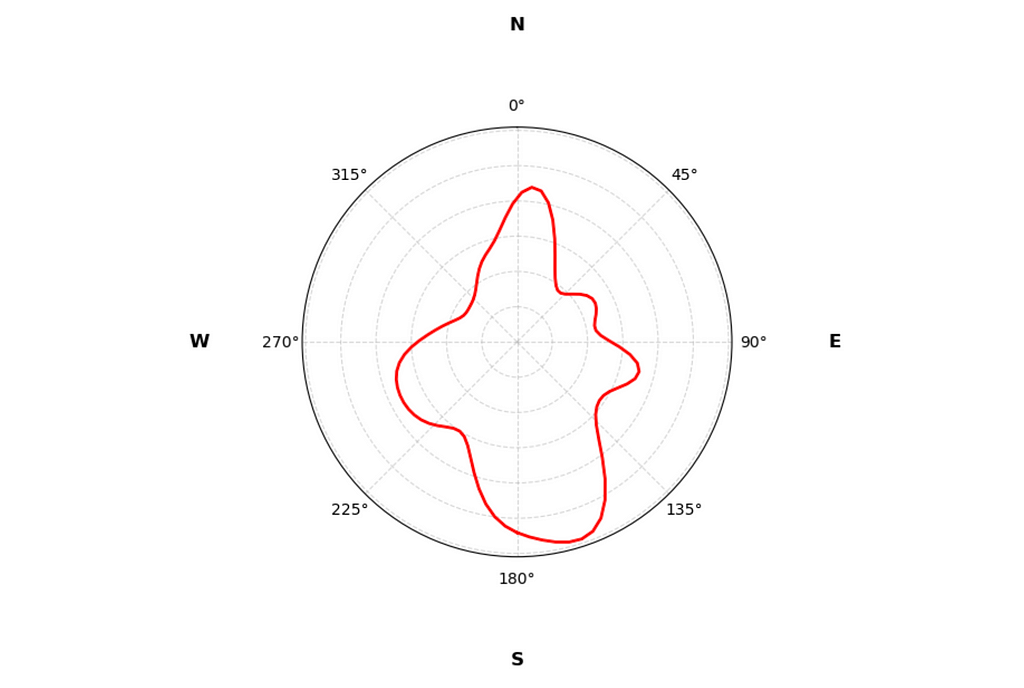
Circular KDE of doggy business (image by author)
With the KDE plot we get a smoother representation of the distribution. And the good news is that it is very far from being a uniform circle.
It’s time to validate it statistically!
Statistically Significant Poops
Just as circular data requires special treatment for visualizations and distributions, it also requires special statistical tests.
I’ll be using a few tests from the pingouin library I already mentioned earlier. The first test I’ll use is the Rayleigh test which is a test for uniformity of circular data. The null hypothesis claims that the data is uniformly distributed around the circle and the alternative is that it is not.
Good news, everyone! The p-value is less than 0.05 and we reject the null hypothesis. Auri’s strategic poop positioning is not random!
The only downside is that the test assumes that the distribution has only one mode and the data is sampled from a von Mises distribution. Oh well, let’s try something else then. Auri’s data clearly has multiple modes.
The next on the list is the V-test. This test checks if the data is non-uniform with a specified mean direction. From the documentation we get that:
The V test has more power than the Rayleigh test and is preferred if there is reason to believe in a specific mean direction.
Perfect! Let’s try it.
From the distribution it’s clear that Auri prefers the South direction above all. I’ll set the mean direction to π radians (South) and run the test.
Now we’re getting somewhere! The p-value is close to zero and we reject the null hypothesis. Auri is a statistically significant South-facing pooper!
Bayesian Poops: Math Part
And now for something completely different. Let’s try a Bayesian approach.
To start, I decided to see how estimate of the mean direction changes as the sample size increased. The idea is simple: I’ll start with a circular uniform prior distribution and update it with every new data point.
We’ll need to define a few things, so let’s get down to math. If you’re not a fan of equations, feel free to skip to the next section with cool visualizations!
1. The von Mises Distribution
The von Mises distribution p(θ∣μ,κ) has a probability density function given by:
where:
μ is the mean direction
κ is the concentration parameter (analogous to the inverse of the variance in a normal distribution)
I₀(κ) is the modified Bessel function of the first kind, ensuring the distribution is normalized
2. Prior and Likelihood
Suppose we have:
Prior distribution:
Likelihood for a new observation θₙ:
We want to update our prior using Bayes’ theorem:
where
3. Multiply the Prior and Likelihood in the von Mises Form
The product of two von Mises distributions with parameters (μ1, κ1) and (μ2, κ2) leads to another von Mises distribution with updated parameters. Let’s go through the steps:
Given:
and
the posterior is proportional to the product:
Using the trigonometric identity for the sum of cosines:
This becomes:
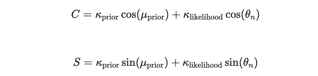
4. Convert to Polar Form for the Posterior
Final stretch! The expression above is a von Mises distribution in disguise. We can rewrite it in the polar form to estimate the updated mean direction and concentration parameter.
Let:
Now the expression for posterior simplifies to:
Let’s pause here and take a closer look at the simplified expression.
Notice that C cos(θ)+S sin(θ) is the dot product of two vectors (C,S) and (cos(θ),sin(θ)) which we can represent as:
where ϕ is the angle between the vectors (C,S) and (cos(θ),sin(θ)).
2. The magnitudes of the vectors are:
3. The angle between the vector (cos(θ),sin(θ)) and a positive x-axis is just θ and between (C,S) and a positive x-axis is, by definition:
4. So the angle between the two vectors is:
Substitute our findings back into the simplified expression for the posterior:
or
where
kappa_post is the posterior concentration parameter:
mu_post is the posterior mean direction
Yay, we made it! The posterior is also a von Mises distribution with updated parameters (mu_post, kappa_post). Now we can update the prior with every new observation and see how the mean direction changes.
Bayesian Poops: Fun Part
Welcome back to those of you who skipped the math and congratulations to those who made it through! Let’s code the Bayesian update and vizualize the results.
First, let’s define the helper functions for visualizing the posterior distribution. We’ll need to it to create a nice animation later on.
import imageio from io import BytesIO
def get_posterior_distribution_image_array( mu_grid: np.ndarray, posterior_pdf: np.ndarray, current_samples: List[float], idx: int, fig_size: Tuple[int, int], dpi: int, r_max_posterior: float ) -> np.ndarray: """ Creates the posterior distribution and observed samples histogram on a polar plot, converts it to an image array, and returns it for GIF processing.
Parameters: -----------
mu_grid (np.ndarray): Grid of mean direction values for plotting the posterior PDF. posterior_pdf (np.ndarray): Posterior probability density function values for the given `mu_grid`. current_samples (List[float]): List of observed angle samples in radians. idx (int): The current step index, used for labeling the plot. fig_size (Tuple[int, int]): Size of the plot figure (width, height). dpi (int): Dots per inch (resolution) for the plot. r_max_posterior (float): Maximum radius for the posterior PDF plot, used to set plot limits.
Returns: np.ndarray: Image array of the plot in RGB format, suitable for GIF processing. """ fig = plt.figure(figsize=fig_size, dpi=dpi) ax = plt.subplot(1, 1, 1, projection='polar') ax.set_theta_zero_location('N') ax.set_theta_direction(-1) ax.plot(mu_grid, posterior_pdf, color='red', linewidth=2, label='Posterior PDF')
# set the maximum radius to accommodate both the posterior pdf and histogram bars r_histogram_height = r_max_posterior * 0.9 r_max = r_max_posterior + r_histogram_height ax.set_ylim(0, r_max)
# plot the histogram bars outside the circle for i in range(len(hist_counts_normalized)): theta = bin_centers[i] width = bin_width hist_height = hist_counts_normalized[i] * r_histogram_height if hist_counts_normalized[i] > 0: ax.bar( theta, hist_height, width=width, bottom=r_max_posterior, color='teal', edgecolor='black', alpha=0.5 )
Now we’re ready to write the update loop. Remember that we need to set our prior distribution. I’ll start with a circular uniform distribution which is equivalent to a von Mises distribution with a concentration parameter of 0. For the kappa_likelihood I set a fixed moderate concentration parameter of 2. That’ll make the posterior update more visible.
# initial prior parameters mu_prior = 0.0 # initial mean direction (any value, since kappa_prior = 0) kappa_prior = 0.0 # uniform prior over the circle
# fixed concentration parameter for the likelihood kappa_likelihood = 2.0
# updating priors for next iteration mu_prior = mu_post kappa_prior = kappa_post
# Create GIF fps = 10 frames.extend([img_array]*fps*3) # repeat last frame a few times to make a "pause" at the end of the GIF imageio.mimsave('../images/posterior_updates.gif', frames, fps=fps)
And that’s it! The code will generate a GIF showing the posterior distribution update with every new observation. Here’s the glorious result:
Posterior Distribution Updates (image by author)
With every new observation the posterior distribution gets more and more concentrated around the true mean direction. If only I could replace the red line with Auri’s silhouette, it would be perfect!
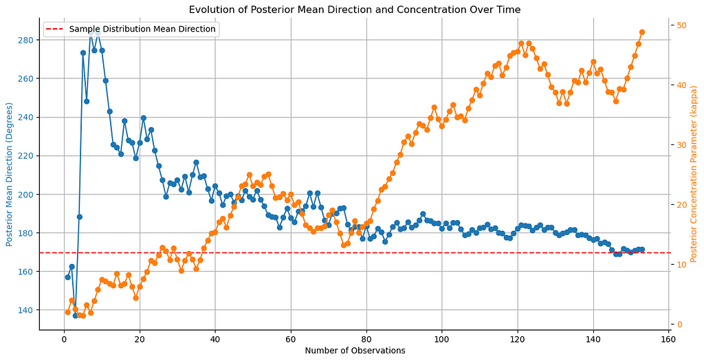
We can further visualize the history of the posterior mean direction and concentration parameter. Let’s plot them:
# Convert posterior_mus to degrees
posterior_mus_deg = np.rad2deg(posterior_mus) % 360
n_samples = data.shape[0]
true_mu = data['degrees'].mean()
# Plot evolution of posterior mean direction
fig, ax1 = plt.subplots(figsize=(12, 6))

color = 'tab:blue'
ax1.set_xlabel('Number of Observations')
ax1.set_ylabel('Posterior Mean Direction (Degrees)', color=color)
ax1.plot(range(1, n_samples + 1), posterior_mus_deg, marker='o', color=color)
ax1.tick_params(axis='y', labelcolor=color)
ax1.axhline(true_mu, color='red', linestyle='--', label='Sample Distribution Mean Direction')
ax1.legend(loc='upper left')
ax1.grid(True)

ax2 = ax1.twinx()  # instantiate a second axes that shares the same x-axis
color = 'tab:orange'
ax2.set_ylabel('Posterior Concentration Parameter (kappa)', color=color)  # we already handled the x-label with ax1
ax2.plot(range(1, n_samples + 1), posterior_kappas, marker='o', color=color)
ax2.tick_params(axis='y', labelcolor=color)

fig.tight_layout()  # otherwise the right y-label is slightly clipped
sns.despine()
plt.title('Evolution of Posterior Mean Direction and Concentration Over Time')
plt.show()
Posterior mu, kappa evolution (image by author)
The plot shows how the posterior mean direction and concentration parameter evolve with every new observation. The mean direction eventually converges to the sample value, while the concentration parameter increases, as the estimate becomes more certain.
Bayes Factor: PyMC for Doggy Compass
The last thing I wanted to try was to use the Bayes Factor approach for hypothesis testing. The idea behind the Bayes Factor is very simple: it’s the ratio of two marginal likelihoods for two competing hypotheses/models.
In general, the Bayes Factor is defined as:
where:
p(D∣Mi) and p(D∣Mj) are the marginal likelihoods of the data under the i and j hypothesis
p(Mi∣D) and p(Mj∣D) are the posterior probabilities of the models given the data
p(Mi) and p(Mj) are the prior probabilities of the models
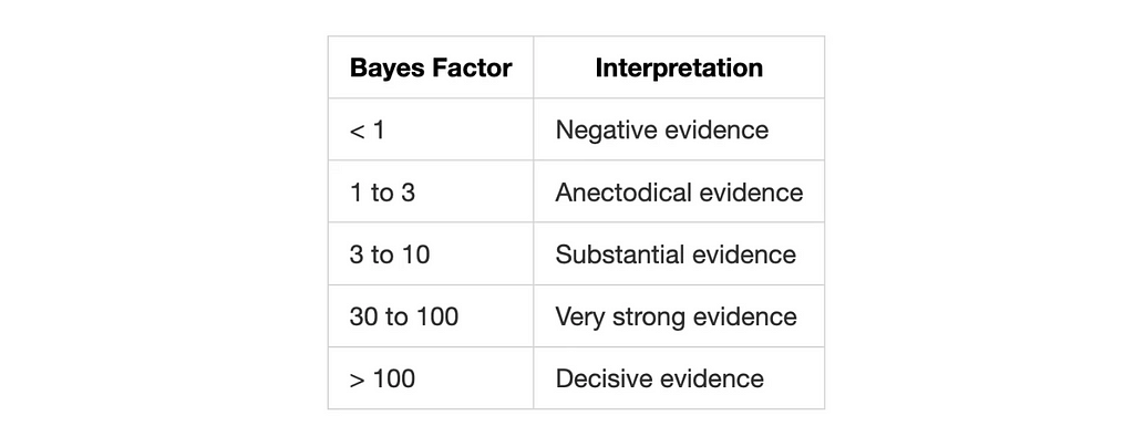
The result is a number that tells us how much more likely one hypothesis is compared to the other. There are different approaches to interpret the Bayes Factor, but a common one is to use the Jeffreys’ scale by Harold Jeffreys:
What are the models you might ask? Simple! They are distributions with different parameters. I’ll be using PyMC to define the models and sample posterior distributions from them.
First of all, let’s re-itroduce the null hypothesis. I still assume it’s a circular uniform Von Mises distribution with kappa=0 but this time we need to calculate the likelihood of the data under this hypothesis. To simplify further calculations, we’ll be calculating log-likelihoods.
Next, it’s time to build the alternative model. Starting with a simple scenario of a Unimodal South direction, where I assume that the distribution is concentrated around 180° or π in radians.
Unimodal South
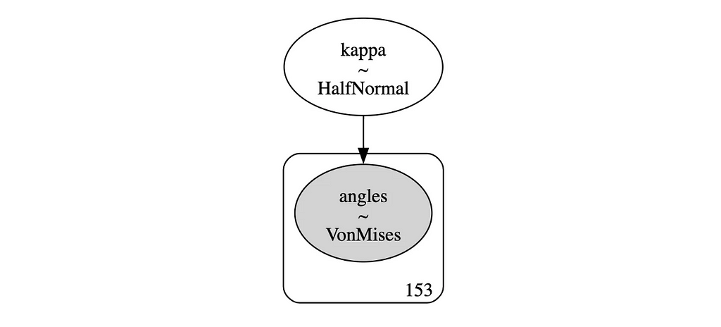
Let’s define the model in PyMC. We’ll use Von Mises distribution with a fixed location parameter μ=π and a Half-Normal prior for the non-negative concentration parameter κ. This allows the model to learn the concentration parameter from the data and check if the South direction is preferred.
import pymc as pm
import arviz as az
import arviz.data.inference_data as InferenceData
from scipy.stats import halfnorm, gaussian_kde

with pm.Model() as model_uni:
    # Prior for kappa
    kappa = pm.HalfNormal('kappa', sigma=10)
    # Likelihood
    likelihood_h1 = pm.VonMises('angles', mu=np.pi, kappa=kappa, observed=data['radians'])
    # Sample from posterior
    trace_uni = pm.sample(
        10000, tune=3000, chains=4,
        return_inferencedata=True,
        idata_kwargs={'log_likelihood': True})
This gives us a nice simple model which we can also visualize:
# Model graph
pm.model_to_graphviz(model_uni)
PyMC model graph (image by author)
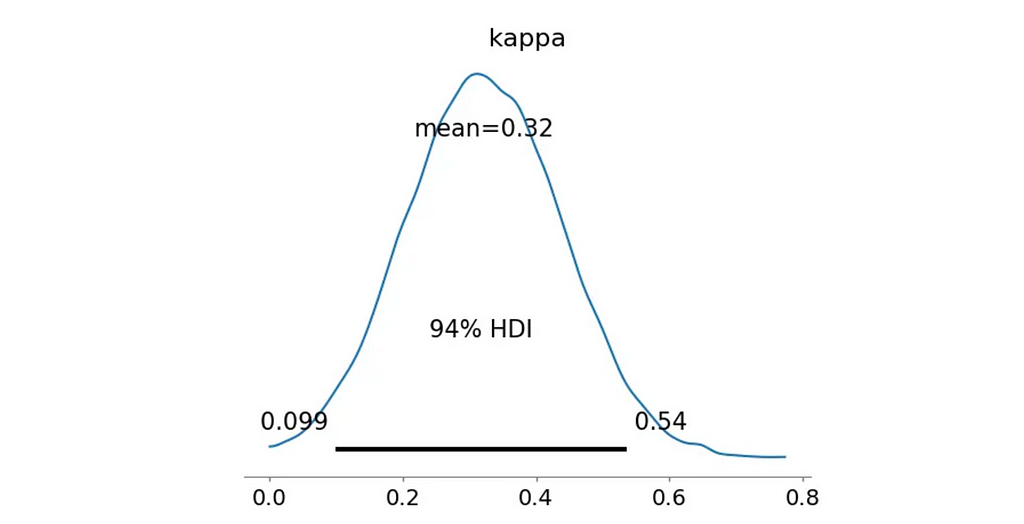
And here’s the posterior distribution for the concentration parameter κ:
All that’s left is to calculate the log-likelihood for the alternative model and the Bayes Factor.
# Posterior samples for kappa
kappa_samples = trace_uni.posterior.kappa.values.flatten()
# Log likelihood for each sample
log_likes = []
for k in kappa_samples:
    # Von Mises log likelihood
    log_like = vonmises.logpdf(data['radians'], k, loc=np.pi).sum()
    log_likes.append(log_like)
# Log-mean-exp trick for numerical stability
log_likelihood_h1 = np.max(log_likes) +
       np.log(np.mean(np.exp(log_likes - np.max(log_likes))))
BF = np.exp(log_likelihood_h1 - log_likelihood_h0)
print(f"Bayes Factor: {BF:.4f}")
print(f"Probability kappa > 0.5: {np.mean(kappa_samples > 0.5):.4f}")
>> Bayes Factor: 32.4645
>> Probability kappa > 0.5: 0.0649
Since we’re dividing the likelihood of the alternative model by the likelihood of the null model, the Bayes Factor indicates how much more likely the data is under the alternative hypothesis. In this case, we get 32.46, a very strong evidence, suggesting that the data is not uniformly distributed around the circle and there is a preference for the South direction.
However, we additionally calculate the probability that the concentration parameter kappa is greater than 0.5. This is a simple way to check if the distribution is significantly different from the uniform one. With the Unimodal South model, this probabiliy is only 0.0649, meaning that the distribution is still quite spread out.
Let’s try another model: Bimodal North-South Mixture.
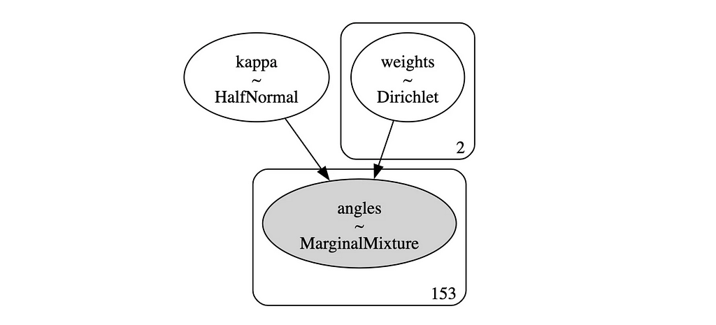
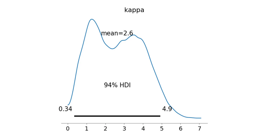
Bimodal North-South Mixture
This time I’ll assume that the distribution is bimodal with peaks around 0° and 180°, just as we’ve seen in the compass rose.
To achieve this, I’ll need a mixture of two Von Mises distributions with different fixed mean directions and a shared concentration parameter.
def compute_mixture_vonmises_logpdf( series: ArrayLike, kappa: float, weights: npt.NDArray[np.float64], mus: List[float] ) -> float: """ Compute log PDF for a mixture of von Mises distributions
Parameters: ----------- series: ArrayLike Array of observed angles in radians kappa: float Concentration parameter weights: npt.NDArray[np.float64], Array of mixture weights mus: List[float] Array of means for each component
Returns: -------- float: Sum of log probabilities for all data points """ mixture_pdf = np.zeros_like(series)
for w, mu in zip(weights, mus): mixture_pdf += w * vonmises.pdf(series, kappa, loc=mu)
""" Generate a report with Bayes Factor and probability kappa > threshold
Parameters: ----------- log_likelihood_h0: float Log likelihood for the null hypothesis log_likelihood_h1: float Log likelihood for the alternative hypothesis kappa_samples: ArrayLike Flattened posterior samples of the concentration parameter kappa_threshold: float Threshold for computing the probability that kappa > threshold
Returns: -------- summary: str A formatted string containing the summary statistics. """ BF = np.exp(log_likelihood_h1 - log_likelihood_h0)
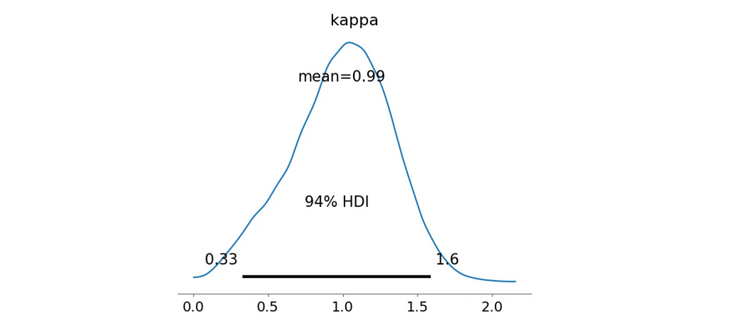
>> Bayes Factor: 214.2333
>> Probability kappa > 0.5: 0.9110
Fantastic! Both our metrics indicate that this model is a much better fit for the data. The Bayes Factor suggests a decisive evidence and most of the posterior κ samples are greater than 0.5 with the mean value of 0.99 as we’ve seen on the distribution plot.
Let’s try a couple more models before wrapping up.
Bimodal West-South Mixture
This model once again assumes a bimodal distribution but this time with peaks around 270° and 180°, which were common directions in the compass rose.
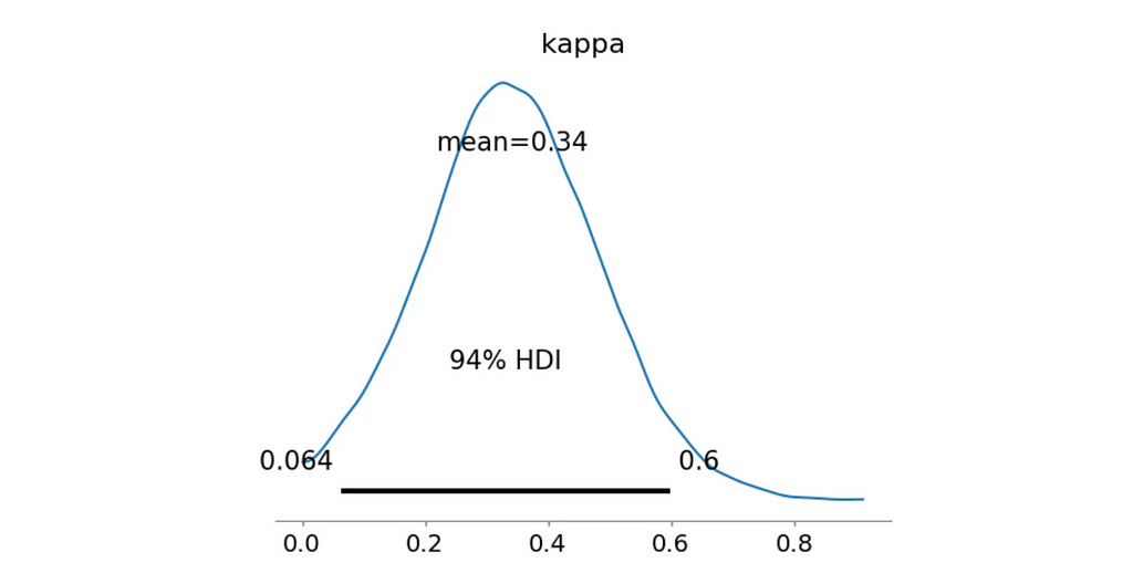
>> Bayes Factor: 20.2361
>> Probability kappa > 0.5: 0.1329
Posterior kappa distribution (image by author)
Nope, definitely not as good as the previous model. Next!
Quadrimodal Mixture
Final round. Maybe my dog really likes to align himself with the cardinal directions? Let’s try a quadrimodal distribution with peaks around 0°, 90°, 180°, and 270°.
>> Bayes Factor: 0.0000
>> Probability kappa > 0.5: 0.9644
Posterior kappa distribution (image by author)
Well… Not really. Although the probability that the concentration parameter κκ is greater than 0.5 is quite high, the Bayes Factor is 0.0.
The great thing about Bayes Factor is that it penalizes overly complex models effectively preventing overfitting.
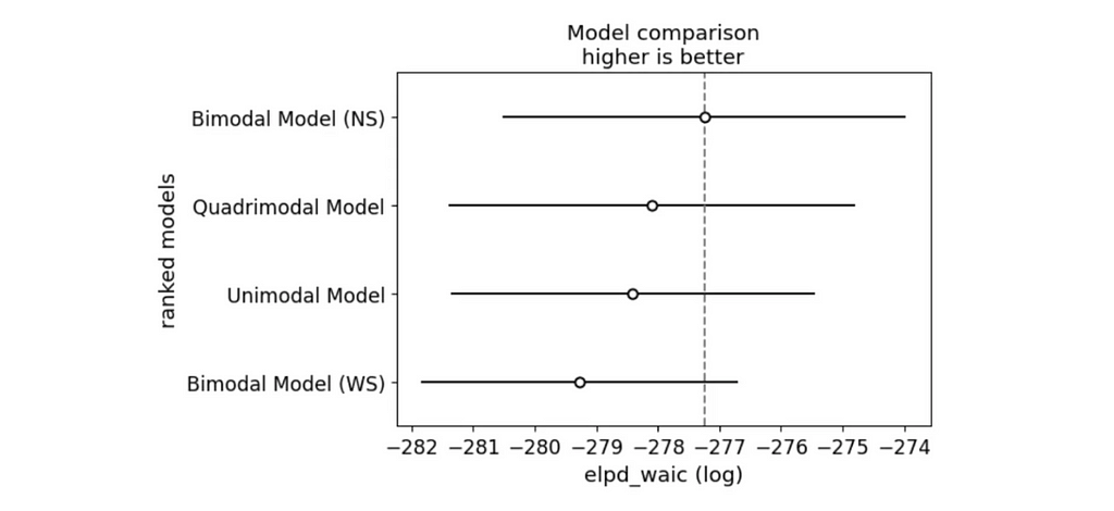
Model Comparison
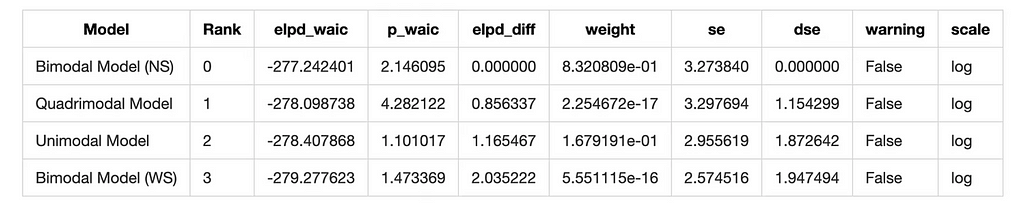
Let’s summarize the results of all models using information criteria. We’ll use the Widely Applicable Information Criterion (WAIC) and the Leave-One-Out Cross-Validation (LOO) to compare the models.
# Compute WAIC for each model
wail_uni = az.waic(trace_uni)
waic_quad = az.waic(trace_mixture_quad)
waic_bimodal_NS = az.waic(trace_mixture_bimodal_NS)
waic_bimodal_WS = az.waic(trace_mixture_bimodal_WS)

model_dict = {
    'Quadrimodal Model': trace_mixture_quad,
    'Bimodal Model (NS)': trace_mixture_bimodal_NS,
    'Bimodal Model (WS)': trace_mixture_bimodal_WS,
    'Unimodal Model': trace_uni
}
# Compare models using WAIC
waic_comparison = az.compare(model_dict, ic='waic')
waic_comparison
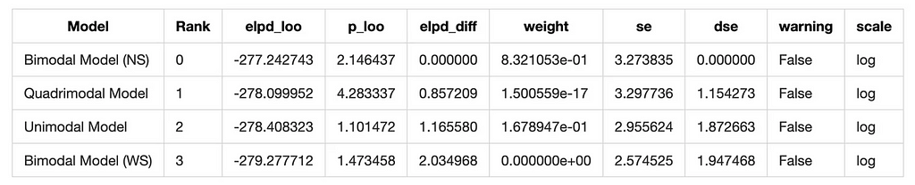
# Compare models using LOO
loo_comparison = az.compare(model_dict, ic='loo')
loo_comparison
# Visualize the comparison
az.plot_compare(waic_comparison)
plt.show()
WAIC comparison (image by author)
And we have a winner! The Bimodal North-South model is the best fit for the data according to both WAIC and LOO.
Conclusion
Christmas Auri (image by author)
What a journey! What started a few months ago as a simple observation of my dog’s pooping habits turned into a full-blown Bayesian analysis.
In this article, I’ve shown how to model circular data, estimate the mean direction and concentration parameter, and update the posterior distribution with new observations. We’ve also seen how to use the Bayes Factor for hypothesis testing and compare models using information criteria.
And the results were super interesting! Auri does indeed have preferences and somehow manages to align himself across the North-South axis. If I ever get lost in the woods with my dog, I know what direction to follow. Just need a big enough sample size to be sure!
I hope you enjoyed this journey as much as I did. If you have any questions or suggestions, feel free to reach out. And if you’d like to support my work, consider buying me a coffee ❤️
Your guide to the web’s new LLM-ready content standard
You might’ve seen various dev tools adding LLMs.txt support to their docs recently. This proposed web standard is quickly gaining adoption, but what is it exactly and why does it matter?
While robots.txt and sitemap.xml are designed for search engines, LLMs.txt is optimized for reasoning engines. It provides information about a website to LLMs in a format they can easily understand.
So, how did LLMs.txt go from proposal to industry trend practically overnight?
On November 14th, Mintlify added LLMs.txt support to their docs platform. In one move, they made thousands of dev tools’ docs LLM-friendly, like Anthropic and Cursor.
Anthropic and others quickly posted on X about their LLMs.txt support. More Mintlify-hosted docs joined in, creating a wave of visibility for the proposed standard.
The momentum sparked new community sites and tools. @ifox created directory.llmstxt.cloud to index LLM-friendly technical docs. @screenfluent followed shortly with llmstxt.directory.
Mot, who made dotenvx, built and shared an open-source generator tool for dotenvx’s docs site. Eric Ciarla of Firecrawl created a tool that scrapes your website and creates the file for you.
Who created LLMs.txt and why?
Jeremy Howard, co-founder of Answer.AI, proposed LLMs.txt to solve a specific technical challenge.
AI systems can only process limited context windows, making it difficult for them to understand large documentation sites. Traditional SEO techniques are optimized for search crawlers rather than reasoning engines, and so they can’t solve this limitation.
When AI systems try to process HTML pages directly, they get bogged down with navigation elements, JavaScript, CSS, and other non-essential info that reduces the space available for actual content.
LLMs.txt solves that by giving the AI the exact information it needs in a format it understands.
What exactly is an LLMs.txt file?
LLMs.txt is a markdown file with a specific structure. The specification defines two distinct files:
/llms.txt: A streamlined view of your documentation navigation to help AI systems quickly understand your site’s structure
/llms-full.txt: A comprehensive file containing all your documentation in one place
/llms.txt
The file must start with an H1 project name, followed by a blockquote summary. Subsequent sections use H2 headers to organize documentation links. The “Optional” section specifically marking less critical resources.
# Project Name
> Brief project summary

Additional context and important notes

## Core Documentation
- [Quick Start](url): Description of the resource
- [API Reference](url): API documentation details

## Optional
- [Additional Resources](url): Supplementary information
For a simple example, see llmtxt.org’s own LLM.txt. For an in-depth, multi-language example, see Anthropic’s.
/llms-full.txt
While /llms.txt provides navigation and structure, /llms-full.txt contains the complete documentation content in markdown.
# AI Review (Beta)
AI Review is a feature that allows you to review your recent changes in your codebase to catch any potential bugs.
You can click into individual review items to see the full context in the editor, and chat with the AI to get more information.
### Custom Review Instructions
In order for AI Review to work in your favor, you can provide custom instructions for the AI to focus on. For example, if you want the AI to focus on performance-related issues, you could put:
``` focus on the performance of my code ```
This way, AI Review will focus on the performance of your code when scanning through your changes.
### Review Options
Currently, you have a several options to choose from to review:
* `Review Working State` * This will review your uncommitted changes. * `Review Diff with Main Branch` * This will review the diff between your current working state and the main branch. * `Review Last Commit` * This will review the last commit you made.
The above snippet is from Cursor’s /llms-full.txt file. See the full file on Cursor’s docs.
LLMs.txt vs sitemap.xml vs robots.txt
It serves a fundamentally different purpose than existing web standards like sitemap.xml and robots.txt.
/sitemap.xml lists all indexable pages, but doesn’t help with content processing. AI systems would still need to parse complex HTML and handle extra info, cluttering up the context window.
/robots.txt suggests search engine crawler access, but doesn’t assist with content understanding either.
/llms.txt solves AI-related challenges. It helps overcome context window limitations, removes non-essential markup and scripts, and presents content in a structure optimized for AI processing.
How to use LLMs.txt with AI systems
Unlike search engines that actively crawl the web, current LLMs don’t automatically discover and index LLMs.txt files.
You must manually provide the file content to your AI system. This can be done by pasting the link, copying the file contents directly into your prompt, or using the AI tool’s file upload feature.
ChatGPT
First, go to that docs’ or /llms-full.txt URL. Copy the contents or URL into your chat. Ask specific questions about what you’d like to accomplish.
A screenshot of using an llms-full.txt file with ChatGPT (Image by author).
Claude
Claude can’t yet browse the web, so copy the contents of that docs’ /llms-full.txt file into your clipboard. Alternatively, you can save it as a .txt file and upload it. Now you can ask any questions you like confident that it has the full, most up-to-date context.
A screenshot of using an llms-full.txt file with Claude (Image by author).
Cursor
Cursor lets you add and index third party docs and use them as context in your chats. You can do this by typing @Docs > Add new doc. A modal will appear and it’s here where you can add a link to the /llms-full.txt file. You will be able to use it as context like any other doc.
To learn more about this feature see Cursor’s @Docs feature.
A screenshot of inputting a llms-full.txt file into Cursor to use as context (Image by author).
How to generate LLMs.txt files
There are several different tools you can use to create your own:
Mintlify: Automatically generates both /llms.txt and /llms-full.txt for hosted documentation
llmstxt by dotenv: A tool by dotenvx’s creator Mot that generates llms.txt using your site’s sitemap.xml.
llmstxt by Firecrawl: A different tool by Firecrawl’s founder, Eric Ciarla, that scrapes your website using Firecrawl to generate the llms.txt file.
What’s next for LLMs.txt?
LLMs.txt represents a shift toward AI-first documentation.
Just as SEO became essential for search visibility, having AI-readable content will become crucial for dev tools and docs.
As more sites adopt this file, we’ll likely see new tools and best practices emerge for making content accessible to both humans and AI assistants.
For now, LLMs.txt offers a practical solution to help AI systems better understand and utilize web content, particularly for technical documentation and APIs.
LLMs.txt Explained was originally published in Towards Data Science on Medium, where people are continuing the conversation by highlighting and responding to this story.
Imagine you are a hungry hiker, lost on a trail away from the city. After walking many miles, you find a road and spot a faint outline of a car coming towards you. You mentally prepare a sympathy pitch for the driver, but your hope turns to horror as you realize the car is driving itself. There is no human to showcase your trustworthiness, or seek sympathy from.
Deciding against jumping in front of the car, you try thumbing a ride, but the car’s software clocks you as a weird pedestrian and it whooses past you.
Sometimes having an emergency call button or a live helpline [to satisfy California law requirements] is not enough. Some edge cases require intervention, and they will happen more often as autonomous cars take up more of our roads. Edge cases like these are especially tricky, because they need to be taken on a case by case basis. Solving them isn’t as easy as coding a distressed face classifier, unless you want people posing distressed faces to get free rides. Maybe the cars can make use of human support, ‘tele-guidance’ as Zoox calls it, to vet genuine cases while also ensuring the system is not taken advantage of, a realistically boring solution that would work… for now. An interesting development in autonomous car research holds the key to a more sophisticated solution.
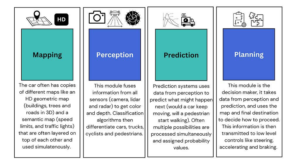
Typically an autonomous driving algorithm works by breaking down driving into modular components and getting good at them. This breakdown looks different in different companies but a popular one that Waymo and Zoox use, has modules for mapping, perception, prediction, and planning.
Figure 1: The base modules that are at the core of traditional self-driving cars. Source: Image by author.
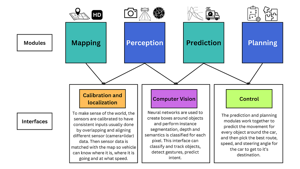
Each of these modules only focus on the one function which they are heavily trained on, this makes them easier to debug and optimize. Interfaces are then engineered on top of these modules to connect them and make them work together.
Figure 2: A simplification of how modules are connected through interfaces. Source: Image by author.
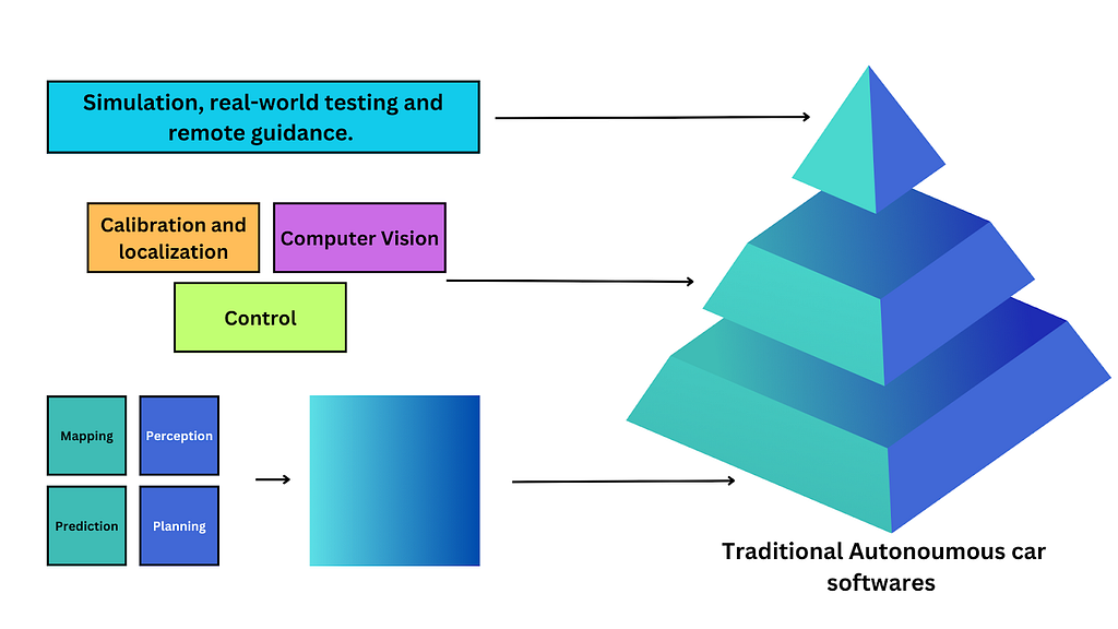
After connecting these modules using the interfaces, the pipeline is then further trained on simulations and tested in the real world.
Figure 3: How the different software pieces in self-driving cars come together. Source: Image by author.
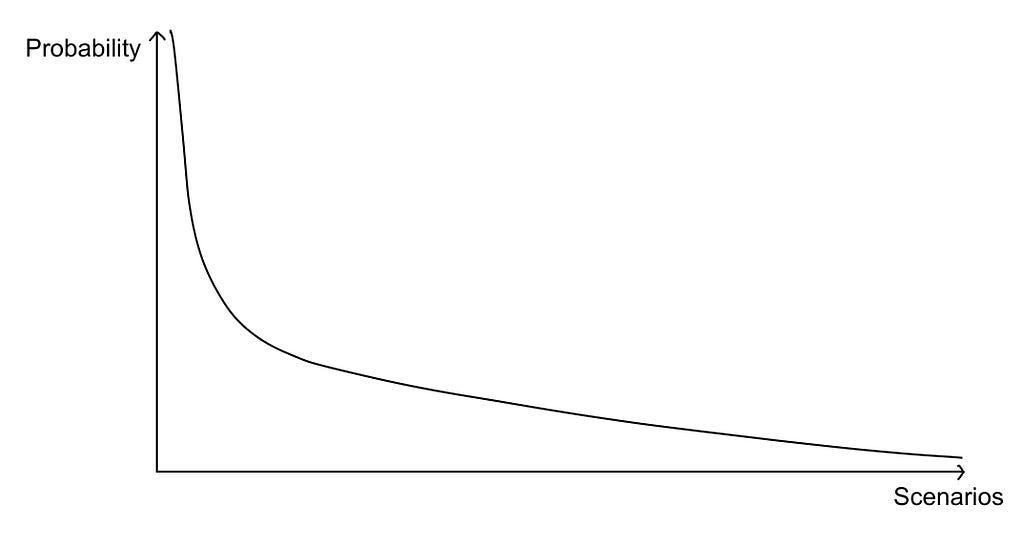
This approach works well, but it is inefficient. Since each module is trained separately, the interfaces often struggle to make them work well together. This means the cars adapt badly to novel environments. Often cumulative errors build up among modules, made worse by inflexible pre-set rules. The answer might seem to just train them on less likely scenarios, which seems plausible intuitively but is actually quite implausible. This is because driving scenarios fall under a long tailed distribution.
Figure 4: A long tail distribution, showcasing that training the car on less likely scenarios gets diminishing marginal returns the further you go. Source: Image by author.
This means we have the most likely scenarios that are easily trained, but there are so many unlikely scenarios that trying to train our model on them is exceptionally computationally expensive and time consuming only to get marginal returns. Scenarios like an eagle nose diving from the sky, a sudden sinkhole formation, a utility pole collapsing, or driving behind a car with a blown brake light fuse. With a car only trained on highly relevant data, with no worldly knowledge, which struggles to adapt to novel solutions, this means an endless catch-up game to account for all these implausible scenarios, or worse, being forced to add more training scenarios when something goes very wrong.
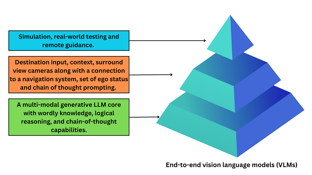
Two weeks ago, Waymo Research published a paper on EMMA, an end-to-end multimodal model which can turn the problem on its head. This end-to-end model instead of having modular components, would include an all knowing LLM with all its worldly knowledge at the core of the model, this LLM would then be further fine-tuned to drive. For example Waymo’s EMMA is built on top of Google’s Gemini while DriveGPT is built on top of OpenAI’s ChatGPT.
This core is then trained using elaborate prompts to provide context and ask questions to deduce its spatial reasoning, road graph estimation, and scene understanding capabilities. The LLMs are also asked to offer decoded visualizations, to analyze whether the textual explanation matches up with how the LLM would act in a simulation. This multimodal infusion with language input makes the training process much more simplified as you can have simultaneous training of multiple tasks with a single model, allowing for task-specific predictions through simple variations of the task prompt.
Figure 5: How an end-to-end Vision Language Model is trained to drive. Source: Image by author.
Another interesting input is often an ego variable, which has nothing to do with how superior the car feels but rather stores data like the car’s location, velocity, acceleration and orientation to help the car plan out a route for smooth and consistent driving. This improves performance through smoother behavior transitions and consistent interactions with surrounding agents in multiple consecutive steps.
These end-to-end models, when tested through simulations, give us a state-of-the-art performance on public benchmarks. How does GPT knowing how to file a 1040 help it drive better? Worldly knowledge and logical reasoning capabilities means better performance in novel situations. This model also lets us co-train on tasks, which outperforms single task models by more than 5.5%, an improvement despite much less input (no HD map, no interfaces, and no access to lidar or radar). They are also much better at understanding hand gestures, turn signals, or spoken commands from other drivers and are socially adept at evaluating driving behaviors and aggressiveness of surrounding cars and adjust their predictions accordingly. You can also ask them to justify their decisions which gets us around their “black box” nature, making validation and traceability of decisions much easier.
In addition to all this, LLMs can also help with creating simulations that they can then be tested on, since they can label images and can receive text input to create images. This can significantly simplify constructing an easily controllable setting for testing and validating the decision boundaries of autonomous driving systems and simulating a variety of driving situations.
This approach is still slower, can input limited image frames and is more computationally extensive but as our LLMs get better, faster, less computationally expensive and incorporate additional modalities like lidar and radar, we will see this multimodal approach surpass specialized expert models in 3D object detection quality exponentially, but that might be a few years down the road.
As end-to-end autonomous cars drive for longer it would be interesting to see how they imprint on the human drivers around them, and develop a unique ‘auto-temperament’ or personality in each city. It would be a fascinating case study of driving behaviours around the world. It would be even more fascinating to see how they impact the human drivers around them.
An end-to-end system would also mean being able to have a conversation with the car, like you converse with ChatGPT, or being able to walk up to a car on the street and ask it for directions. It also means hearing less stories from my friends, who vow to never sit in a Waymo again after it almost ran into a speeding ambulance or failed to stop for a low flying bird.
Imagine an autonomous car not just knowing where it is at what time of day (on a desolate highway close to midnight) but also understanding what that means (the pedestrian is out of place and likely in trouble). Imagine a car not just being able to call for help (because California law demands it) but actually being the help because it can logically reason with ethics. Now that would be a car that would be worth the ride.
References:
Chen, L., Sinavski, O., Hünermann, J., Karnsund, A., Willmott, A. J., Birch, D., Maund, D., & Shotton, J. (2023). Driving with LLMs: Fusing Object-Level Vector Modality for Explainable Autonomous Driving (arXiv:2310.01957). arXiv. https://doi.org/10.48550/arXiv.2310.01957
Cui, C., Ma, Y., Cao, X., Ye, W., Zhou, Y., Liang, K., Chen, J., Lu, J., Yang, Z., Liao, K.-D., Gao, T., Li, E., Tang, K., Cao, Z., Zhou, T., Liu, A., Yan, X., Mei, S., Cao, J., … Zheng, C. (2024). A Survey on Multimodal Large Language Models for Autonomous Driving. 2024 IEEE/CVF Winter Conference on Applications of Computer Vision Workshops (WACVW), 958–979. https://doi.org/10.1109/WACVW60836.2024.00106
Fu, D., Lei, W., Wen, L., Cai, P., Mao, S., Dou, M., Shi, B., & Qiao, Y. (2024). LimSim++: A Closed-Loop Platform for Deploying Multimodal LLMs in Autonomous Driving (arXiv:2402.01246). arXiv. https://doi.org/10.48550/arXiv.2402.01246
Hwang, J.-J., Xu, R., Lin, H., Hung, W.-C., Ji, J., Choi, K., Huang, D., He, T., Covington, P., Sapp, B., Zhou, Y., Guo, J., Anguelov, D., & Tan, M. (2024). EMMA: End-to-End Multimodal Model for Autonomous Driving (arXiv:2410.23262). arXiv. https://doi.org/10.48550/arXiv.2410.23262
The ‘full-stack’: Behind autonomous driving. (n.d.). Zoox. Retrieved November 26, 2024, from https://zoox.com/autonomy
Wang, B., Duan, H., Feng, Y., Chen, X., Fu, Y., Mo, Z., & Di, X. (2024). Can LLMs Understand Social Norms in Autonomous Driving Games? (arXiv:2408.12680). arXiv. https://doi.org/10.48550/arXiv.2408.12680
Wang, Y., Jiao, R., Zhan, S. S., Lang, C., Huang, C., Wang, Z., Yang, Z., & Zhu, Q. (2024). Empowering Autonomous Driving with Large Language Models: A Safety Perspective (arXiv:2312.00812). arXiv. https://doi.org/10.48550/arXiv.2312.00812
Xu, Z., Zhang, Y., Xie, E., Zhao, Z., Guo, Y., Wong, K.-Y. K., Li, Z., & Zhao, H. (2024). DriveGPT4: Interpretable End-to-end Autonomous Driving via Large Language Model (arXiv:2310.01412). arXiv. https://doi.org/10.48550/arXiv.2310.01412
Yang, Z., Jia, X., Li, H., & Yan, J. (n.d.). LLM4Drive: A Survey of Large Language Models for Autonomous Driving.
In this post, we present a generative AI-powered semantic search solution that empowers business users to quickly and accurately find relevant data assets across various enterprise data sources. In this solution, we integrate large language models (LLMs) hosted on Amazon Bedrock backed by a knowledge base that is derived from a knowledge graph built on Amazon Neptune to create a powerful search paradigm that enables natural language-based questions to integrate search across documents stored in Amazon Simple Storage Service (Amazon S3), data lake tables hosted on the AWS Glue Data Catalog, and enterprise assets in Amazon DataZone.
We use cookies on our website to give you the most relevant experience by remembering your preferences and repeat visits. By clicking “Accept”, you consent to the use of ALL the cookies.
This website uses cookies to improve your experience while you navigate through the website. Out of these, the cookies that are categorized as necessary are stored on your browser as they are essential for the working of basic functionalities of the website. We also use third-party cookies that help us analyze and understand how you use this website. These cookies will be stored in your browser only with your consent. You also have the option to opt-out of these cookies. But opting out of some of these cookies may affect your browsing experience.
Necessary cookies are absolutely essential for the website to function properly. These cookies ensure basic functionalities and security features of the website, anonymously.
Cookie
Duration
Description
cookielawinfo-checkbox-analytics
11 months
This cookie is set by GDPR Cookie Consent plugin. The cookie is used to store the user consent for the cookies in the category "Analytics".
cookielawinfo-checkbox-functional
11 months
The cookie is set by GDPR cookie consent to record the user consent for the cookies in the category "Functional".
cookielawinfo-checkbox-necessary
11 months
This cookie is set by GDPR Cookie Consent plugin. The cookies is used to store the user consent for the cookies in the category "Necessary".
cookielawinfo-checkbox-others
11 months
This cookie is set by GDPR Cookie Consent plugin. The cookie is used to store the user consent for the cookies in the category "Other.
cookielawinfo-checkbox-performance
11 months
This cookie is set by GDPR Cookie Consent plugin. The cookie is used to store the user consent for the cookies in the category "Performance".
viewed_cookie_policy
11 months
The cookie is set by the GDPR Cookie Consent plugin and is used to store whether or not user has consented to the use of cookies. It does not store any personal data.
Functional cookies help to perform certain functionalities like sharing the content of the website on social media platforms, collect feedbacks, and other third-party features.
Performance cookies are used to understand and analyze the key performance indexes of the website which helps in delivering a better user experience for the visitors.
Analytical cookies are used to understand how visitors interact with the website. These cookies help provide information on metrics the number of visitors, bounce rate, traffic source, etc.
Advertisement cookies are used to provide visitors with relevant ads and marketing campaigns. These cookies track visitors across websites and collect information to provide customized ads.