Lost in a maze of datasets and endless data dictionaries? Say goodbye to tedious variable hunting! Discover how to quickly identify and extract the variables you need from multiple SAS files using two simple R functions. Streamline your workflow, save time, and make data preparation a breeze!
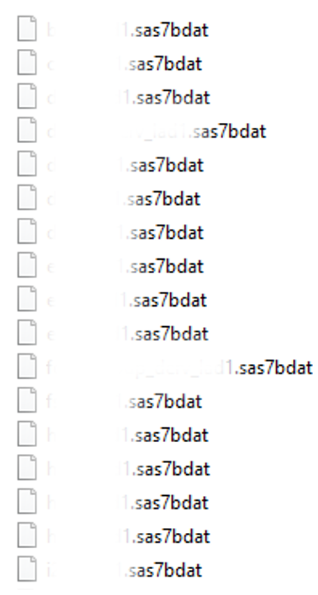
As a researcher with over seven years of experience working with health data, I’ve often been handed folders full of datasets. For example, imagine opening a folder containing 56 SAS files, each with unique data (example below). If you’ve been in this situation, you know the frustration: trying to locate a specific variable in a sea of files feels like looking for a needle in a haystack.
Screenshot taken by the author of a local folder. File names have been blurred to maintain the confidentiality of the datasets.
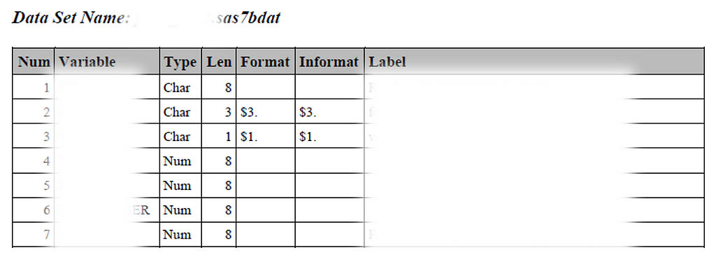
At first glance, this may not seem like an issue if you already know where your variables of interest are. But often, you don’t. While a data dictionary is usually provided, it’s frequently a PDF document that lists variables across multiple pages. Finding what you need might involve searching (Ctrl+F) for a variable on page 100, only to realize the dataset’s name is listed on page 10. Scrolling back and forth wastes time.
Screenshot taken by the author of a data dictionary. Variable names and labels have been blurred to maintain the confidentiality of the datasets.
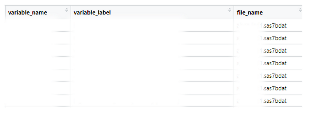
To save myself from this tedious process, I created a reproducible R workflow to read all datasets in a folder, generate a consolidated dataframe of variable names and their labels (example below), and identify where each variable is located. This approach has made my work faster and more efficient. Here’s how you can do it, step by step.
Screenshot taken by the author of of how the names_labels dataset looks like (see step 2). Variable names and labels have been blurred to maintain the confidentiality of the datasets.
Step-by-Step Guide
Step 1: Use the get_names_labels Function
First, use the custom function get_names_labels (code provided at the end of this post). This function requires the folder path where all your datasets are stored.
The get_names_labels function will create a dataframe named names_labels (like the example above), which includes:
· Variable name (variable_name)
· Variable label (variable_label)
· The name of the dataset(s) where the variable was found (file_name)
Depending on the number and size of the datasets, this process may take a minute or two.
Step 3: Search for Variables
Once the names_labels dataframe is generated, you can search for the variables you need. Filter the variable_name or variable_label columns to locate relevant terms. For example, if you’re looking for gender-related variables, they might be labeled as sex, gender, is_male, or is_female.
Be mindful that similar variables might exist in multiple datasets. For instance, age could appear in the main questionnaire, a clinical dataset, and a laboratory dataset. These variables might look identical but differ based on how and where the data was collected. For example:
· Age in the main questionnaire: Collected from all survey participants.
· Age in clinical/lab datasets: Limited to a subset invited for further assessments or those who agreed to participate.
In such cases, the variable from the main questionnaire might be more representative of the full population.
Step 4: Identify Relevant Datasets
Once you’ve determined which variables you need, filter the names_labels dataframe to identify the original datasets (file_name) containing them. If a variable appears in multiple datasets (e.g., ID), you’ll need to identify which dataset includes all the variables you’re interested in.
# Say you want these two variables
variables_needed <- c('ID', 'VAR1_A')
names_labels <- names_labels[which(names_labels$variable_name %in% variables_needed), ]
If one of the variables can be found in multiple original datasets (e.g., ID), you will filter names_labels to keep only the original dataset with both variables (e.g., ID and VAR1_A). In our case, the names_labels dataframe will be reduced to only two rows, one for each of the two variables we were looking for, both of which will be found in the same original dataset.
Now, use the read_and_select function (provided at the end). Pass the name of the original dataset containing the variables of interest. This function creates a new dataframe in your R environment with only the selected variables. For example, if your variables are in ABC.sas7bdat, the function will create a new dataframe called ABC with just those variables.
unique(names_labels$file_name) # Sanity check, that there is only one dataframe
read_and_select(unique(names_labels$file_name)[1])
Step 6: Clean Your Environment
To keep your workspace tidy, remove unnecessary elements and retain only the new dataframe(s) you need. For example, if your variables of interest came from ABC.sas7bdat, you’ll keep the filtered dataframe ABC which was the output of the read_and_select function.
If your variables of interest are in more than one dataset (e.g., ABC and DEF), you can merge them. Use a unique identifier, such as ID, to combine the datasets into a single dataframe. The result will be a unified dataframe with all the variables you need. You will get a df dataframe with all the observations and only the variables you needed.
# Get a list with the names of the dataframes in the environment (“ABC” and “DEF”)
object_names <- ls()


# Get a list with the actual dataframe
object_list <- mget(object_names)


# Reduce the dataframes in the list (“ABC” and “DEF”) by merging conditional on the unique identifier (“ID”)
df <- Reduce(function(x, y) merge(x, y, by = "ID", all = TRUE), object_list)

# Clean your environment to keep only the dataframes (“ABC” and “DEF”) and a new dataframe “df” which will contain all the variables you needed.
rm(object_list, object_names)
Why This Workflow Works?
This approach saves time and organizes your work into a single, reproducible script. If you later decide to add more variables, simply revisit steps 2 and 3, update your list, and rerun the script. This flexibility is invaluable when dealing with large datasets. While you’ll still need to consult documentation to understand variable definitions and data collection methods, this workflow reduces the effort required to locate and prepare your data. Handling multiple datasets doesn’t have to be overwhelming. By leveraging my custom functions like get_names_labels and read_and_select, you can streamline your workflow for data preparation.
Have you faced similar challenges when working with multiple datasets? Share your thoughts or tips in the comments, or give this article a thumbs up if you found it helpful. Let’s keep the conversation going and learn from each other!
Below are the two custom functions. Save them in an R script file, and load the script into your working environment whenever needed. For example, you could save the file as _Functions.R for easy access.
# You can load the functions as
source('D:/Folder1/Folder2/Folder3/_Functions.R')
## STEPS TO USE THESE FUNCTIONS: ## 1. DEFINE THE OBJECT 'PATH_FILE', WHICH IS A PATH TO THE DIRECTORY WHERE ## ALL THE DATASETS ARE STORED. ## 2. APPLY THE FUNCTION 'get_names_labels' WITH THE PATH. THE FUNCTION WILL ## RETURN A DATAFRAME NAMES 'names_labels'. ## 3. THE FUNCTION WILL RETURN A DATASET ('names_labels) SHOWING THE NAMES OF ## THE VARIABLES, THE LABELS, AND THE DATASET. VISUALLY/MANUALLY EXPLORE THE ## DATASET TO SELECT THE VARIABLES WE NEED. CREATE A VECTOR WITH THE NAMES ## OF THE VARIABLES WE NEED, AND NAME THIS VECTOR 'variables_needed'. ## 4. FROM THE DATASET 'names_labels', KEEP ONLY THE ROWS WITH THE VARIABLES WE ## WILL USE (STORED IN THE VECTOR 'variables_needed'). ## 5. APPLY THE FUNCTION 'read_and_select' TO EACH OF THE DATASETS WITH RELEVANT ## VARIABLES. THIS FUNCTION WILL ONLY NEED THE NAME OF THE DATASET, WHICH IS ## STORED IN THE LAST COLUMN OF DATASET 'names_labels'.
### FUNCTION TO 1) READ ALL DATASETS IN A FOLDER; 2) EXTRACT NAMES AND LABELS; ### 3) PUT NAMES AND LABELS IN A DATASET; AND 4) RETURN THE DATASET. THE ONLY ### INPUT NEEDED IS A PATH TO A DIRECTORY WHERE ALL THE DATASETS ARE STORED.
### FUNCTION TO READ EACH DATASET AND KEEP ONLY THE VARIABLES WE SELECTED; THE ### FUNCTION WILL SAVE EACH DATASET IN THE ENVIRONMENT. THE ONLY INPUNT IS THE ### NAME OF THE DATASET.
Background licensed from elements.envato.com, edit by Marcel Müller 2024
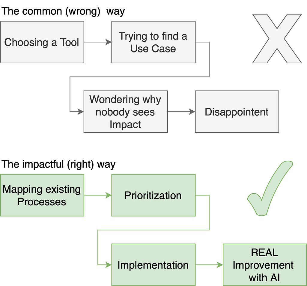
The most common disillusion that many organizations have is the following: They get excited about generative AI with ChatGPT or Microsoft Co-Pilot, read some article about how AI can “make your business better in some way,” then try to find other use cases where they can slap a chatbot on and in the end are disappointed when the results are not super satisfying. And then, the justification phase comes. I often hear things like, “The model is not good enough” or “We need to upskill the people to write better prompts.”
In 90% of the cases, these are not the correct conclusions and come from the issue that we think in Chatbots. I have developed over three dozen generative AI applications for organizations of three people to global enterprises with over three hundred thousand employees and I have seen this pattern everywhere.
There are thousands of companies out there telling you that you need to have “some kind of chatbot solution” because everybody does that. OpenAI with ChatGPT, Microsoft Copilot, Google with Gemini and all the other companies selling you chatbots are doing a great job breaking down initial barriers to creating a chatbot. But let me tell you: 75% of the really painful problems you can solve with generative AI do not benefit from being a chatbot.
Too often, I see managers, program directors, or other decision-makers start with the idea: “We have here some product with AI that lets us build chatbots — let’s find as many places as possible to implement it.” In my experience, this is the wrong approach because you are starting from a solution and trying to fit an existing problem into it. What would be the correct way would be to look into a problem, analyze it and find an AI solution that fits. A chatbot may be a good interface for some use cases, but forcing every issue into a chatbot is problematic.
In this article, I’ll share insights and the method I’ve developed through hands-on experience building countless applications. These applications, now live in production and serving thousands of users, have shaped my thinking about building impactful generative AI solutions — instead of blindly following a trend and feeling disappointed if it does not work.
Think about your Processes first — Chatbots (or other interfaces) second
I tell you not to start your thinking from chatbots, so where should you start? The answer is simple: business processes.
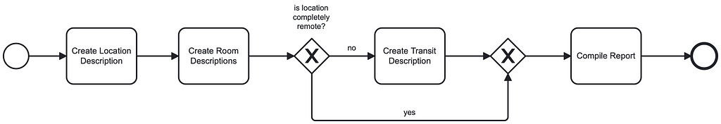
Everything that happens within a company is a business process. A business process is a combination of different activities (“units of work”), events (for example, errors), and gateways (for example, decisions) connected into a workflow [1]. There are tools for modeling business processes [2] in well-known diagram forms and a whole research discipline centered around analyzing and improving business processes [3][4][5]. Business Process Management is a good tool because it is not theoretical but is used everywhere in companies — even though they do not know what to call it.
Let me give you an example. Imagine you are a company that does real estate valuations for a bank. Before banks give out mortgages, they ask real estate valuers to estimate how much the object is worth so that they know that in case the mortgage cannot be paid back, they have the actual price.
Creating a real estate valuation report is one large business process we can break down into subprocesses. Usually, valuers physically drive to the house, take pictures and then sit there writing a 20–30 page report describing their valuation. Let us, for a moment, not fall into the “uh a 20–30 page report, let me sit in front of ChatGPT and I will probably be faster” habit. Remember: processes first, then the solution.
We can break this process down into smaller sub-processes like driving to the house, taking pictures and then writing the different parts of the report: location description of the house, describing the condition and sizes of the different rooms. When we look deeper into a single process, we will see the tasks, gateways, and events involved. For example, for writing the description of the location, a real estate valuer sits at their desk, does some research, looks on Google Maps what shops are around, and checks out the transport map of the city to determine how well the house is connected and how the street looks like. These are all activities (or tasks) that the case worker has to do. If the home is a single farm in the middle of nowhere, the public transport options are probably irrelevant because buyers of such houses usually are car dependent anyway. This decision on which path to go in a process is called a gateway.
This process-driven mindset we apply here starts with assessing the current process before throwing any AI on it.
Orchestration Instead of Chat-Based Interactions
With this analysis of our processes and our goal we can now start looking into how a process with AI should look like. It is important to think about the individual steps that we need to take. If we only focus on the subprocess for creating the description that may look like this:
analyzing the locations and shops around the house
describing the condition of the interior
unless the location is very remote: finding the closest public transport stops
writing a page of text for the report
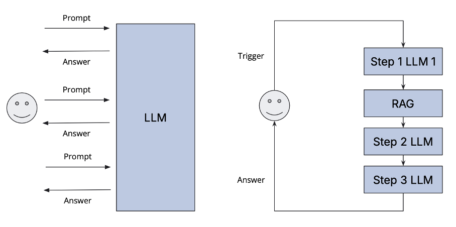
And yes, you can do that in an interactive way with a chatbot where you work with an “AI sparring partner” until you have your output. But this has in a company setting three major issues:
Reproducibility: Everybody prompts differently. This leads to different outputs depending on the skill and experience level of the prompting user. As a company, we want our output to be as reproducible as possible.
Varying quality: You probably have had interactions with ChatGPT where you needed to rephrase prompts multiple times until you had the quality that you wanted. And sometimes you get completely wrong answers. In this example, we have not found a single LLM that can describe the shops around in high quality without hallucinating.
Data and existing systems integration: Every company has internal knowledge that they might want to use in those interactions. And yes, you can do some retrieval augemented generation (RAG) with chatbots, but it is not the easiest and most universal approach that leads to good results in each case.
Those issues come from the core foundation that LLMs behind chatbots have.
Instead of relying on a “prompt-response” interaction cycle, enterprise applications should be designed as a series of orchestrated, (partially) AI-driven process steps, each targeting a specific goal. For example, users could trigger a multi-step process that integrates various models and potentially multimodal inputs to deliver more effective results and combine those steps with small scripts that retrieve data without using AI. More powerful and automated workflows can be created by incorporating Retrieval-Augmented Generation (RAG) and minimizing human intervention.
This orchestration approach delivers significant efficiency improvements compared to manual orchestration through an interactive interface. Also, not every step in the process should be done by relying purely on an AI model. In the example above, we actually discovered that using the Google Maps API to get nearby stops and transit stations is far superior in terms of quality than asking a good LLM like GPT-4o or even a web search RAG engine like Perplexity.
Efficiency Gains Through Orchestration
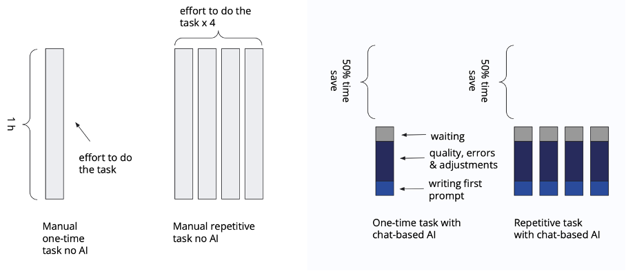
Let us think for a moment about a time without AI. Manual processes can take significant time. Let’s assume a task takes one hour to complete manually, and the process is repeated four times, requiring four hours in total. Using a chatbot solution powered by generative AI could save 50% (or whatever percentage) of the time. However, the remaining time is spent formulating prompts, waiting for responses, and ensuring output quality through corrections and adjustments. Is that as good as it gets?
For repetitive tasks, despite the time savings, the need to formulate prompts, wait, and adjust outputs for consistency can be problematic in organizations where multiple employees execute the same process. To address this, leveraging process templates becomes critical.
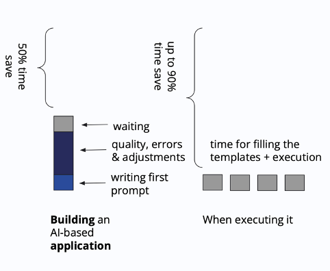
With templates, processes are generalized and parametrized to be reusable. The effort to create a high-quality process template occurs only once, while the execution for individual cases becomes significantly more efficient. Time spent on prompt creation, quality assurance, and output adjustments is dramatically reduced. This is the core difference when comparing chatbot-based solutions to AI-supported process orchestration with templates. And this core difference has a huge impact on quality and reproducibility.
Also, we now have a narrow field where we can test and validate our solution. In a chatbot where the user can insert anything, testing and finding confidencein a quantifiable way is hard. The more we define and restrict the possible parameters and files a user can insert, the better we can validate a solution quantitatively.
Using templates in AI-supported processes mirrors the principles of a Business Process Engine in traditional process management. When a new case arises, these engines utilize a repository of templates and select the corresponding template for orchestration. For orchestration, the input parameters are then filled.
In our example case of the real estate evaluation process, our template has three inputs: The type of object (single-family home), a collection of pictures of the interior and the address.
The process template looks like this:
Use the Google Places API with the given address to find the shops around.
Use the OpenAI vision API to describe the interior conditions.
Use the Google Places API to find the closest transport options.
Take the output JSON objects from 1. and 3. and the description of the transport options and create a page of text with GPT-4o with the following structure: Description of the object, shops and transport, then followed by the interior description and a conclusion giving each a score.
In our example use case, we have implemented the application using the entAIngine platform with the built-in no-code builder.
Note that in this process, only 1 out of 4 steps uses a large language model. And that is something good! Because the Google Maps API never hallucinates. Yes, it can have outdated data, but it will never “just make something up that sounds like it could be a reality.” Second, we have verifiability for a human in the loop because now we have real sources of information that we can analyze and sign off on.
In traditional process management, templates reduce process variability, ensure repeatability, and enhance efficiency and quality (as seen in methodologies like Six Sigma). This is the same mindset we have to adopt here.
Interfaces for Generative AI Applications
Now, we have started with a process that uses an LLM but also solves a lot of headaches. But how does a user interact with it?
The implementation of such a process can work by coding everything manually or by using a No-Code AI process engine like entAIngine [6].
When using templates to model business processes, interactions can occur in various ways. According to my experience in the last 2 years, for 90% of generative AI use cases, the following interfaces are relevant:
• Knowledge Retrieval Interface: Functions like a search engine that can cite and reference sources.
• Document Editor Interface: Combines text processing with access to templates, models, and orchestrations.
• Chat Interface: For iterative, interactive engagement.
• Embedded Orchestration without a Dedicated Interface (RPA): Integrates into existing interfaces via APIs.
The question in the end is, what is the most efficient way of interacting? And yes, for some creative use cases or for non-repetitive tasks, a chat interface can be the tool of choice. But often, it is not. Often, the core goal of a user is to create some sort of document. Then, having those templates available in an editor interface is a very efficient way of interacting. But sometimes, you do not need to create another isolated interface if you have an existing application that you want to augment with AI. The challenge here is merely to execute the right process, get the input data for it in the existing application, and show the output somewhere in the application interface.
These mentioned interfaces here form the foundation for the majority of generative AI use cases that I have encountered so far and, at the same time, enable scalable integration into enterprise environments.
The Bottom Line
By getting their minds away from “How can I use an AI chatbot everywhere?” to “What processes do which steps and how can generative AI be utilized in those steps?” businesses create the foundation for real AI impact. Combine AI with existing systems and then only look into the type of user interface that you need. In that way, you can unlock efficiency that businesses that cannot think beyond chatbots never even dream of.
References
[1] Dumas et al., “Fundamentals of Business Process Management”, 2018
[2] Object Management Group. “Business Process Model and Notation (BPMN) Version 2.0.2.” OMG Specification, Jan. 2014
[3] van der Aalst, “Process Mining: Data Science in Action”, 2016
[4] Luthra, Sunil, et al. “Total Quality Management (TQM): Principles, Methods, and Applications.” 1st ed., CRC Press, 2020.
[5] Panagacos, “The Ultimate Guide to Business Process Management”, 2012
Generative AI (GenAI) opens the door to faster development cycles, minimized technical and maintenance efforts, and innovative use cases that before seemed out of reach. At the same time, it brings new risks — like hallucinations, and dependencies on third-party APIs.
For Data Scientists and Machine Learning teams, this evolution has a direct impact on their roles. A new type of AI project has appeared, with part of the AI already implemented by external model providers (OpenAI, Anthropic, Meta…). Non-AI-expert teams can now integrate AI solutions with relative ease. In this blog post we’ll discuss what all this means for Data Science and Machine Learning teams:
A wider variety of problems can now be solved, but not all problems are AI problems
Traditional ML is not dead, but is augmented through GenAI
Some problems are best solved with GenAI, but still require ML expertise ro run evaluations and mitigate ethical risks
AI literacy becoming more important within companies, and how Data Scientists play a key role to make it a reality.
A wider variety of problems can now be solved — but not all problems are AI problems
GenAI has unlocked the potential to solve a much broader range of problems, but this doesn’t mean that every problem is an AI problem. Data Scientists and AI experts remain key to identifying when AI makes sense, selecting the appropriate AI techniques, and designing and implementing reliable solutions to solve the given problems (regardless of the solution being GenAI, traditional ML, or a hybrid approach).
However, while the width of AI solutions has grown, two things need to be taken into consideration to select the right use cases and ensure solutions will be future-proof:
At any given moment GenAI models will have certain limitations that might negatively impact a solution. This will always hold true as we are dealing with predictions and probabilities, that will always have a degree of error and uncertainty.
At the same time, things are advancing really fast and will continue to evolve in the near future, decreasing and modifying the limitations and weaknesses of GenAI models and adding new capabilities and features.
If there are specific issues that current LLM versions can’t solve but future versions likely will, it might be more strategic to wait or to develop a less perfect solution for now, rather than to invest in complex in-house developments to overwork and fix current LLMs limitations. Again, Data Scientists and AI experts can help introduce the sensibility on the direction of all this progress, and differentiate which things are likely to be tackled from the model provider side, to the things that should be tackled internally. For instance, incorporating features that allow users to edit or supervise the output of an LLM can be more effective than aiming for full automation with complex logic or fine-tunings.
With GenAI solutions, Data Science teams might need to focus less on the model development part, and more on the whole AI system.
Traditional ML is not dead — but is augmented through GenAI
While GenAI has revolutionized the field of AI and many industries, traditional ML remains indispensable. Many use cases still require traditional ML solutions (take most of the use cases that don’t deal with text or images), while other problems might still be solved more efficiently with ML instead of with GenAI.
Far from replacing traditional ML, GenAI often complements it: it allows faster prototyping and experimentation, and can augment certain use cases through hybrid ML + GenAI solutions.
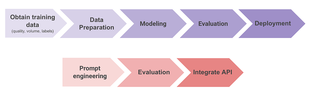
In traditional ML workflows, developing a solution such as a Natural Language Processing (NLP) classifier involves: obtaining training data (which might include manually labelling it), preparing the data, training and fine-tuning a model, evaluating performance, deploying, monitoring, and maintaining the system. This process often takes months and requires significant resources for development and ongoing maintenance.
By contrast, with GenAI, the workflow simplifies dramatically: select the appropriate Large Language Model (LLM), prompt engineering or prompt iteration, offline evaluation, and use an API to integrate the model into production. This reduces greatly the time from idea to deployment, often taking just weeks instead of months. Moreover, much of the maintenance burden is managed by the LLM provider, further decreasing operational costs and complexity.
ML vs GenAI project phases, image by author
For this reason, GenAI allows testing ideas and proving value quickly, without the need to collect labelled data or invest in training and deploying in-house models. Once value is proven, ML teams might decide it makes sense to transition to traditional ML solutions to decrease costs or latency, while potentially leveraging labelled data from the initial GenAI system. Similarly, many companies are now moving to Small Language Models (SMLs) once value is proven, as they can be fine-tuned and more easily deployed while achieving comparable or superior performances compared to LLMs (Small is the new big: The rise of small language models).
In other cases, the optimal solution combines GenAI and traditional ML into hybrid systems that leverage the best of both worlds. A good example is“Building DoorDash’s product knowledge graph with large language models”, where they explain how traditional ML models are used alongside LLMs to refine classification tasks, such as tagging product brands. An LLM is used when the traditional ML model isn’t able to confidently classify something, and if the LLM is able to do so, the traditional ML model is retrained with the new annotations (great feedback loop!).
Either way, ML teams will continue working on traditional ML solutions, fine-tune and deployment of predictive models, while acknowledging how GenAI can help augment the velocity and quality of the solutions.
Some problems will be better solved with GenAI
The AI field is shifting from using numerous in-house specialized models to a few huge multi-task models owned by external companies. ML teams need to embrace this change and be ready to include GenAI solutions in their list of possible methods to use to stay competitive. Although the model training phase is already done, there is the need to maintain the mindset and sensibility around ML and AI as solutions will still be probabilistic, very different from the determinism of traditional software development.
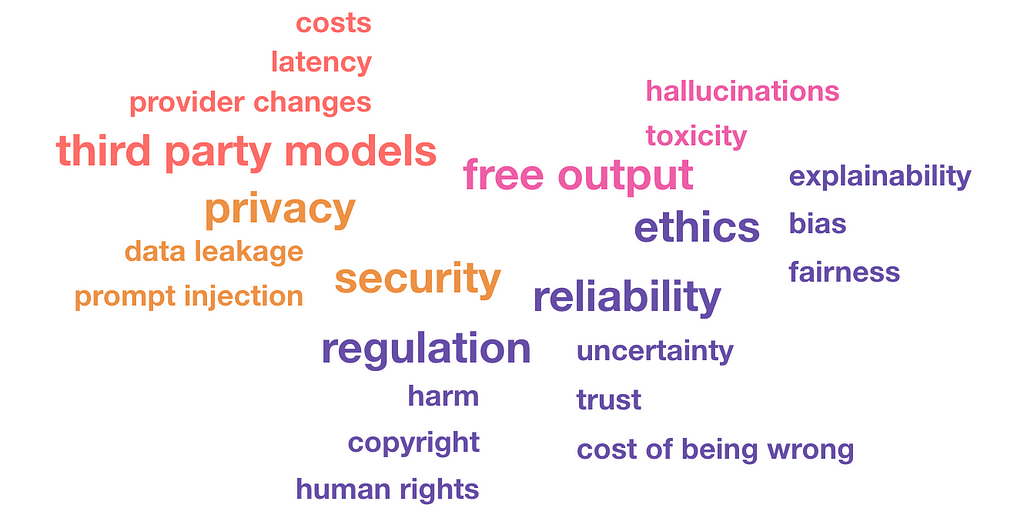
Despite all the benefits that come with GenAI, ML teams will have to address its own set of challenges and risks. The main added risks when considering GenAI-based solutions instead of in-house traditional ML-based ones are:
New GenAI risks are added to the traditional ML risks (in purple), image by autor
Dependency on third-party models: This introduces new costs per call, higher latency that might impact the performance of real-time systems, and lack of control (as we have now limited knowledge of its training data or design decisions, and provider’s updates can introduce unexpected issues in production).
GenAI-Specific Risks: we are well aware of the free input / free output relationship with GenAI. Free input introduces new privacy and security risks (e.g. due to data leakage or prompt injections), while free output introduces risks of hallucination, toxicity or an increase of bias and discrimination.
But still require ML expertise to run evaluations and mitigate ethical risks
While GenAI solutions often are much easier to implement than traditional ML models, their deployment still demands ML expertise, specially in evaluation, monitoring, and ethical risk management.
Just as with traditional ML, the success of GenAI relies on robust evaluation. These solutions need to be assessed from multiple perspectives due to their general “free output” relationship (answer relevancy, correctness, tone, hallucinations, risk of harm…). It is important to run this step before deployment (see picture ML vs GenAI project phases above), usually referred to as “offline evaluation”, as it allows one to have an idea of the behavior and performance of the system when it will be deployed. Make sure to check this great overview of LLM evaluation metrics, which differentiates between statistical scorers (quantitative metrics like BLEU or ROUGE for text relevance) and model-based scorers (e.g., embedding-based similarity measures). DS teams excel in designing and evaluating metrics, even when these metrics can be kind of abstract (e.g. how do you measure usefulness or relevancy?).
Once a GenAI solution is deployed, monitoring becomes critical to ensure that it works as intended and as expected over time. Similar metrics to the ones mentioned for evaluation can be checked in order to ensure that the conclusions from the offline evaluation are maintained once the solution is deployed and working with real data. Monitoring tools like Datadog are already offering LLM-specific observability metrics. In this context, it can also be interesting to enrich the quantitative insights with qualitative feedback, by working close to User Research teams that can help by asking users directly for feedback (e.g. “do you find these suggestions useful, and if not, why?”).
The bigger complexity and black box design of GenAI models amplifies the ethical risks they can carry. ML teams play a crucial role bringing their knowledge about trustworthy AI into the table, having the sensibility about things that can gor wrong, and identifying and mitigating these risks. This work can include running risk assessments, choosing less biased foundational models (ComplAI is an interesting new framework to evaluate and benchmark LLMs on ethical dimensions), defining and evaluating fairness and no-discrimination metrics, and applying techniques and guardrails to ensure outputs are aligned with societal and the organization’s values.
AI Literacy is becoming more important within companies
A company’s competitive advantage will depend not just on its AI internal projects but on how effectively its workforce understands and uses AI. Data Scientists play a key role in fostering AI literacy across teams, enabling employees to leverage AI while understanding its limitations and risks. With their help, AI should act not just as a tool for technical teams but as a core competency across the organization.
To build AI literacy, organizations can implement various initiatives, led by Data Scientists and AI experts like internal trainings, workshops, meetups and hackathons. This awareness can later help:
Augment internal teams and improve their productivity, by encouraging the use of general-purpose AI or specific AI-based features in tools the teams are already using.
Identifying opportunities of great potential from within the teams and their expertise. Business and product experts can introduce great project ideas on topics that were previously dismissed as too complex or impossible (and that might realize are now viable with the help of GenAI).
Wrapping it up: the ever Evolving Role of Data Scientists
It is indisputable that the field of Data Science and Artificial Intelligence is changing fast, and with it the role of Data Scientists and Machine Learning teams. While it’s true that GenAI APIs enable teams with little ML knowledge to implement AI solutions, the expertise of DS and ML teams remains of big value for robust, reliable and ethically sound solutions. The re-defined role of Data Scientists under this new context includes:
Staying up to date with AI progress, to be able to choose the best technique to solve a problem, design and implement a great solution, and make solutions future-proof while acknowledging limitations.
Adopting a system-wide perspective, instead of focusing solely on the predictive model, becoming more end-to-end and including collaboration with other roles to influence how users will interact (and supervise) the system.
Continue working on traditional ML solutions, while acknowledging how GenAI can help augment the velocity and quality of the solutions.
Deep understanding of GenAI limitations and risks, to build reliable and trustworthy AI systems (including evaluation, monitoring and risk management).
Act as AI Champion across the organization: to promote AI literacy and help non-technical teams leverage AI and identify the right opportunities.
The role of Data Scientists is not being replaced, it is being redefined. By embracing this evolution it will remain indispensable, guiding organizations toward leveraging AI effectively and responsibly.
Looking forward to all the opportunities that will come from GenAI and the Data Scientist role redefinition!
The Intuition behind Concordance Index — Survival Analysis
Ranking accuracy versus absolute accuracy
Taken by the author and her Border Collie. “Be thankful for what you have. Be fearless for what you want”
How long would you keep your Gym membership before you decide to cancel it? or Netflix if you are a series fan but busier than usual to allocate 2 hours of your time to your sofa and your TV? Or when to upgrade or replace your smartphone ? What best route to take when considering traffic, road closure, time of the day? or How long until your car needs servicing? These are all regular (but not trivial) questions we face (some of them) in our daily life without thinking too much (or nothing at all) of the thought process we go through on the different factors that influence our next course of action. Surely (or maybe after reading these lines) one would be interested to know what factor or factors could have the greatest influence on the expected time until a given event (from the above or any other for that matter) occurs? In statistics, this is referred as time-to-event-analysis or Survival analysis. And this is the focus of this study.
In Survival Analysis one aims to analyze the time until an event occurs. In this article, I will be employing survival analysis to predict when a registered member is likely to leave (churn), specifically the number of days until a member cancels his/her membership contract. As the variable of interest is the number of days, one key element to explicitly reinforce at this point: the time to event dependent variable is of a continuous type, a variable that can take any value within a certain range. For this, survival analysis is the one to employ.
DATA
This study was conducted using a proprietary dataset provided by a private organization in the tutoring industry. The data includes anonymized records for confidentiality purposes collected over a period of 2 years, namely July 2022 to October 2024. All analyses were conducted in compliance with ethical standards, ensuring data privacy and anonymity. Therefore, to respect the confidentiality of the data provider, any specific organizational details and/or unique identifier details have been omitted.
The final dataset after data pre-processing (i.e. tackling nulls, normalizing to handle outliers, aggregating to remove duplicates and grouping to a sensible level) contains a total of 44,197 records at unique identifier level. A total of 5 columns were input into the model, namely: 1) Age, 2) Number of visits, 3) First visit 4) and Last visit during membership and 5) Tenure. The later representing the number of days holding a membership hence the time-to-event target variable. The visit-based variables are a feature engineered product for this study generated from the original, existing variables and by performing some calculations and aggregation on the raw data for each identifier over the period under analysis. Finally and very importantly, the dataset is ONLY composed of uncensored records. This is, all unique identifiers have experienced the event by the time of the analysis, namely membership cancellation. Therefore there is no censored data in this analysis where individuals survived (did not cancel their membership) beyond their observed duration. This is key when selecting the modelling technique as I will explain next.
Among all different techniques used in survival analysis, three stand out as most commonly used:
Kaplan-Meier Estimator.
This is a non-parametric model hence no assumptions on the distribution of the data is made.
KM is not interested on how individual features affect churn thus it does not offer feature-based insights.
It is widely used for exploratory analysis to assess what the survival curve looks like.
Very importantly, it does not provide personalized predictions.
Cox Proportional Hazard (PH) Model
The Cox PH Model is a semi-parametric model so it does not assume any specific distribution of the survival time, making it more flexible for a wider range of data.
It estimates the hazard function.
It relies heavily on uncensored as well as censored data to be able to differentiate between individuals “at risk” of experiencing the event versus those who already had the event. Thus, if only uncensored data is analyzed the model assumes all individuals experienced the event yielding bias results thus leading the Cox PH to perform poorly.
AFT Model
It does not require censor data. Thus, can be used where everyone has experienced the event.
It directly models the relationship between covariates.
Used when time-to-event outcomes are of primary interest.
The model estimate the time-to-event explicitly. Thus, provide direct predictions on the duration until cancellation.
Given the characteristics of the dataset used in this study, I have selected the Accelerated Failure Time (AFT) Model as the most suitable technique. This choice is driven by two key factors: (1) the dataset contains only uncensored data, and (2) the analysis focuses on generating individual-level predictions for each unique identifier.
Now before diving any deeper into the methodology and model output, I will cover some key concepts:
Survival Function: It provides insight into the likelihood of survival over time
Hazard Function: Rate at which the event is taking place at point in time t. It captures how the event is changing over time.
Time-to-event: Refers to the (target) variable capturing the time until an event occurs.
Censoring: Flag referring to those event that have not occurred yet for some of the subjects within the timeframe of the analysis. NOTE: In this piece of work only uncensored data is analyzed, this is the survival time for all the subjects under the study is known.
Concordance Index: A measure of how well the model predicts the relative ordering of survival time. It is a measure of ranking accuracy rather than absolute accuracy that assess the proportion of all pairs of subjects whose predicted survival time align with the actual outcome.
Akaike Information Criterion (AIC): A measure that evaluates the quality of a model penalizing against the number of irrelevant variables used. When comparing several models, the one with the lowest AIC is considered the best.
Next, I will expand on the first two concepts.
In mathematical terms:
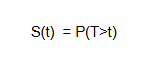
The survival function is given by:
(1)
where,
T is a random variable representing the time to event — duration until the event occurs.
S(t) is the probability that the event has not yet occurred by time t.
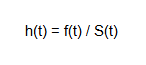
The Hazard function on the other hand is given by:
(2)
where,
f(t) is the probability density function (PDF), which describes the rate at which the event occurs at time t.
S(t) is the survival function that describes the probability of surviving beyond time t
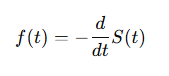
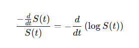
As the PDF f(t) can be expressed in terms of the survival function by taking the derivative of S(t) with respect to t:
(3)
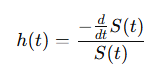
substituting the derivative of S(t) in the hazard function:
(4)
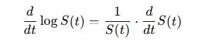
taking the derivative of the Log Survival Function:
(5)
from the chain rule of differentiation it follows:
(6)
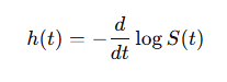
thus, the relationship between the Hazard and Survival function is defined as follow:
(7)
the hazard rate captures how quickly the survival probability changes at a specific point in time.
The Hazard function is always non-negative, it can never go below zero. The shape can increase, decrease, stay constant or vary in more complex forms.
Simply put, the hazard function is a measure of the instantaneous risk of experiencing the event at a point in time t. It tells us how likely is the subject to experience the event right then. The survival (rate) function, on the other hand, measures the probability of surviving beyond a given point in time. This is the overall probability of no experiencing the event up to point in time t.
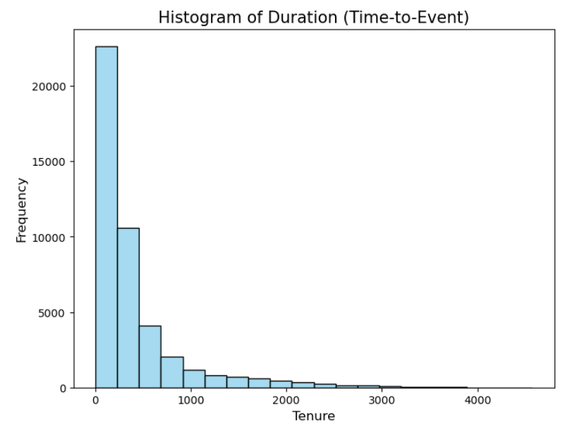
The survival function is always decreasing over time as more and more individuals experience the event. This is illustrated in the below histogram plotting the time-to-event variable: Tenure.
Generated by the author by plotting the time-to-event target variable from the dataset under study.
At t=0, no individual has experienced the event (no individual have cancel their membership yet), thus
(8)
Eventually all individuals experience the event so the survival function tends to zero (0).
(9)
MODEL
For the purposes of this article, I will be focusing on a Multivariate parametric-based model: The Accelerated Failure Time (AFT) model, which explicitly estimate the continuous time-to-event target variable.
Given the AFT Model:
(10)
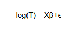
Taking the natural logarithm on both sides of the equation results in:
(11)
where,
log(T) is the logarithm of the survival time, namely time-to-event (duration), which as shown by equation (11) is a linear function of the covariates.
X is the vector of covariates
β is the vector of regression coefficients.
and this is very important:
The coefficients β in the model describe how the covariates accelerate or decelerate the event time, namely the survival time. In an AFT Model (the focus of this piece), the coefficients affect directly the survival time (not the hazard function), specifically:
if β > 1 survival time is longer hence leading to a deceleration of the time to event. This is, the member will take longer to terminate his(her) membership (experiencing the event later).
if β < 1 survival time is shorter hence leading to an acceleration of the time to event. This is, the member will terminate his(her) membership earlier (experiencing the event sooner).
finally,
ϵ is the random error term that represents unobserved factors that affect the survival time.
Now, a few explicit points based on the above:
this is a Multivariate approach, where the time-to-event (duration) target variable is fit on multiple covariates.
a Parametric approach as the model holds an assumption regarding a particular shape of the survival rate distribution.
three algorithms sitting under the AFT model umbrella have been implemented. These are:
3.1) Weibull AFT Model
The model is flexible and can capture different patterns of survival. Supports consistently monotonic increasing/decreasing function. This is: at any two points as defined by the function, the later point is at least as high as the earliest point.
One does not need to explicitly model the hazard function. The model has two parameters from which the survival function is derived: shape, which determines the shape of the distribution hence helps to determine the skewness of the data and scale which determines the spread of the distribution. This PLUS a regression coefficient related to each covariate. The shape parameter dictates the monotonic behaviors of the hazard function, which in turns affects the behavior of the survival function.
Right-skewed, left-skewed distributions of the time-to-event target variable are example of these.
3.2) LogNormal AFT Model
Focuses on modelling the log-transformed of survival time. Logarithm of a random variable whose continuous probability distribution is approximately normally distributed.
Supports right-skewed distributions of the time-to-event target variable. Allows for non-monotonic hazard functions. Useful when the risk of the event does not follow a simple pattern.
It does not require to explicitly model the hazard function.
Two main parameters (plus any regression coefficients): scale and location, the former representing the standard deviation of the log-transformed survival time, the later representing the mean of the log-transformed survival time. This represent the intercept when no covariates are included, otherwise representing the linear combination of these.
3.3) Generalized Gamma AFT Model.
Good fit for a wide range of survival data patterns. Highly adaptable parametric model that accommodates for the above mentioned shapes as well as more complicated mathematical forms on the survival function.
It can be used to test if simpler models (i.e. Weibull, logNormal) can be used instead as it encompasses these as special cases.
It does not require to specify the hazard function.
It has three parameters apart from the regression coefficient ones: shape, scale and location, the later corresponding to the log of the median of survival time when covariates are not included thus the intercept in the model.
TIP: There is a significant amount of literature on these algorithms that specifically focus on each of these algorithms and their features which I strongly suggest the reader to get an understanding on.
Lastly, the performance of the above algorithms is analyzed focusing on the Concordance Index (yes, the C-Index, our metric of interest) and The Akaike Information Criterion (AIC). These are shown next with the models’ output:
REGRESSION OUTPUTS
Weibull AFT Model
Generated by the author employing lifelines library
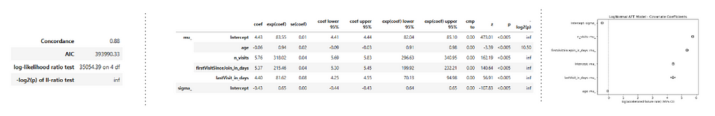
Log Normal AFT Model
Generated by the author employing lifelines library
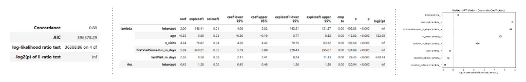
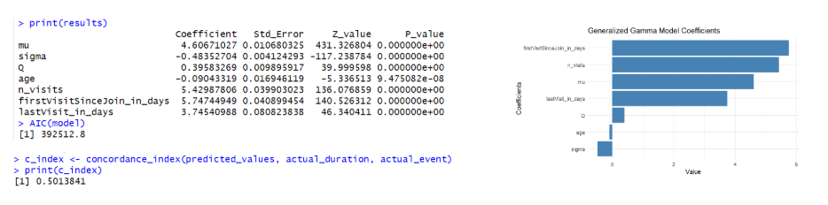
Generalized Gamma AFT Model
Generated by the author employing flexsurv library
On the right hand side, the graphs for each predictor are shown: plotting the log accelerated failure rate on the x axis hence their positive/negative (accelerate/decelerate respectively) impact on the survival time. As shown, all models concur across predictors on the direction of the effect on the survival time providing a consistent conclusion about the predictors positive or negative impact. Now, in terms of The Concordance Index and AIC, the LogNormal and Weibull are both shown with the highest C-Index value BUT specifically the LogNormal Model dominating due to a lower AIC. Thus, the LogNormal is selected as the model with the best fit.
Focusing on the LogNormal AFT Model and interpretation of the estimated coefficient for each covariate (coef), in general predictors are all shown with a p-value lower than the conventional threshold 5% significance level hence rejecting the Null Hypothesis and proving to have a statistical significant impact on the survival time. Age is shown with a negative coefficient -0.06 indicating that as age increases, the member is more likely to experience the event sooner hence terminating his(her) membership earlier. This is: each additional year of age represents a 6% decrease in survival time when the later is multiplied by a factor of 0.94 (exp(coef)) hence accelerating the survival time. In contrast, number of visits, first visit since joined and last visit are all shown with a strong positive effect on survival indicating a strong association between, more visits, early engagement and recent engagement increasing survival time.
Now, in terms of The Concordance Index across models (the focus of this analysis), the Generalized Gamma AFT Model is the one with the lowest C-index value hence the model with the weakest predictive accuracy. This is the model with the weakest ability to correctly rank survival times based on the predicted risk scores. This highlights an important aspect about model performance: regardless of the model ability to capture the correct direction of the effect across predictors, this does not necessarily guarantee predictive accuracy, specifically the ability to discriminate across subjects who experience the event sooner versus later as measured by the concordance index. The C-index explicitly evaluates ranking accuracy of the model as opposed to absolute accuracy. This is a fundamental distinction lying at the heart of this analysis, which I will expand next.
CONCORDANCE INDEX (C-INDEX)
A “ranked survival time” refers to the predicted risk scores produced by the model for each individual and used to rank hence discriminate individuals who experience the event earlier when compared to those who experience the event later. Concordance Index is a measure of ranking accuracy rather than absolute accuracy, specifically: the C-index assesses the proportion of all pairs of individuals whose predicted survival time align with the actual outcome. In absolute terms, there is no concern on how precise the model is on predicting the exact number of days it took for the member to cancel its membership, instead how accurate the model ranks individuals when the actual and predicted time it took for a member to cancel its membership align. The below illustrate this:
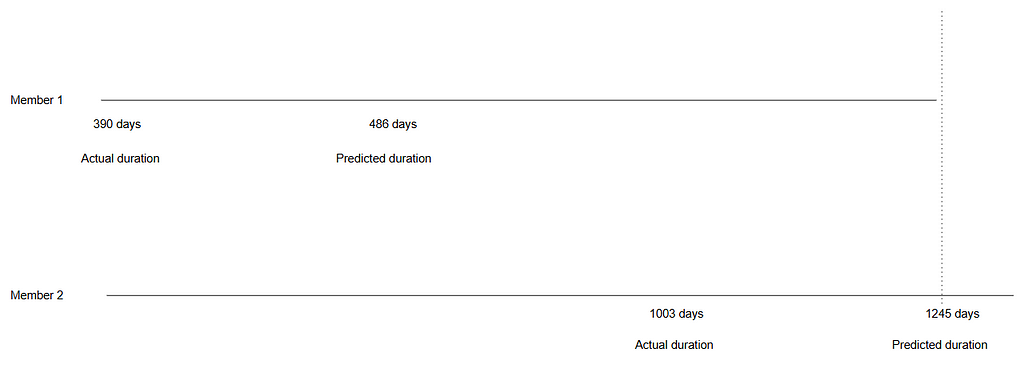
Drawn by the author based on instances: actual and estimate values from the validation dataset.
The two instances above are taken from the validation set after the model was trained on the training set and predictions were generated for unseen data. These examples illustrate cases where the predicted survival time (as estimated by the model) exceeds the actual survival time. The horizontal parallel lines represent time.
For Member 1, the actual membership duration was 390 days, whereas the model predicted a duration of 486 days — an overestimation of 96 days. Similarly, Member 2’s actual membership duration was 1,003 days, but the model predicted the membership cancellation to occur 242 days later than it actually did, this is 1,245 days membership duration.
Despite these discrepancies in absolute predictions (and this is important): the model correctly ranked the two members in terms of risk, accurately predicting that Member 1 would cancel their membership before Member 2. This distinction between absolute error and relative ranking is a critical aspect of model evaluation. Consider the following hypothetical scenario:
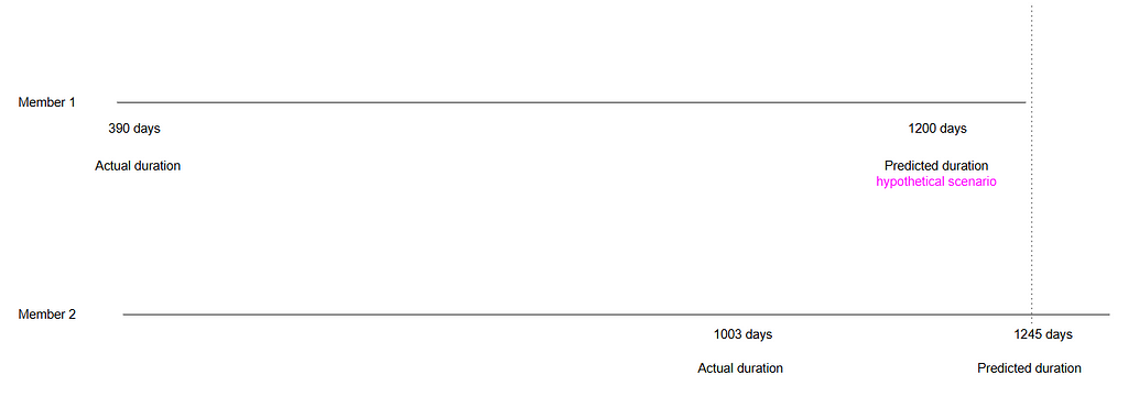
Drawn by the author based on instances: actual and estimate values from the validation dataset.
if the model had predicted a membership duration of 1,200 days for Member 1 instead of 486 days, this would not affect the ranking. The model would still predict that Member 1 terminates their membership earlier than Member 2, regardless of the magnitude of the error in the prediction (i.e., the number of days). In survival analysis, any prediction for Member 1 that falls before the dotted line in the graph would maintain the same ranking, classifying this as a concordant pair. This concept is central to calculating the C-index, which measures the proportion of all pairs that are concordant in the dataset.
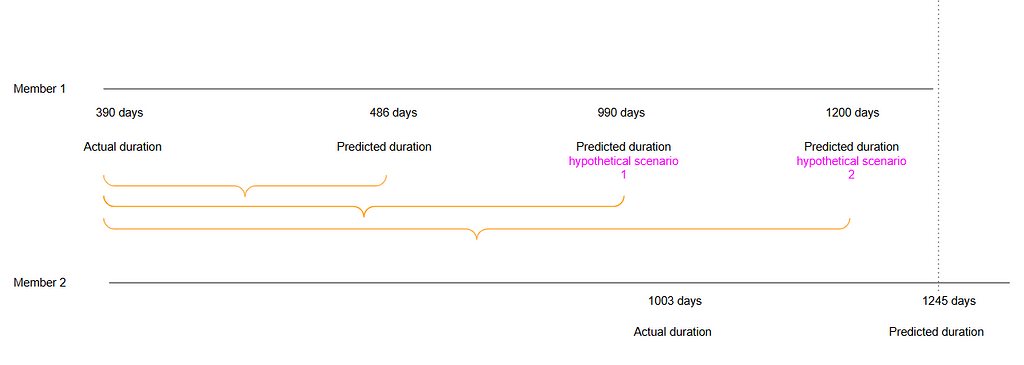
A couple of hypothetical scenarios are shown below. In each of them, the magnitude of the error increases/decreases, namely the difference between the actual event time and the predicted event time, this is the absolute error. However, the ranking accuracy remains unchanged.
Drawn by the author based on instances: actual and estimate values from the validation dataset.
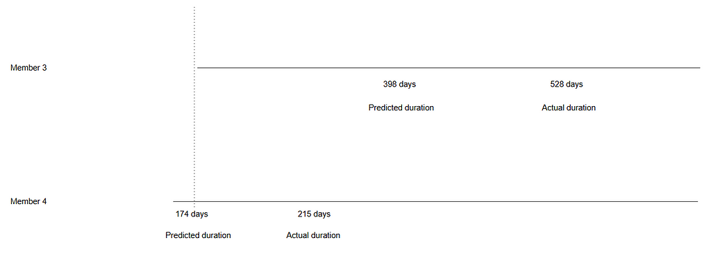
The below are also taken from the validation set BUT for these instances the model predicts the termination of the membership before the actual event occurs. For Member 3, the actual membership duration is 528 days, but the model predicted termination 130 days earlier, namely 398 membership duration. Similarly, for Member 4, the model anticipates the termination of membership before the actual event. In both cases, the model correctly ranks Member 4 to terminate their membership before Member 3.
Drawn by the author based on instances: actual and estimate values from the validation dataset.
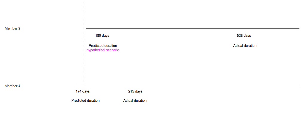
In the hypothetical scenario below, even if the model had predicted the termination 180 days earlier for Member 3, the ranking would remain unchanged. This would still be classified as a concordant pair. We can repeat this analysis multiple times and in 88% of cases, the LogNormal Model will produce this result, as indicated by the concordance index. This is: where the model correctly predicts the relative ordering of the individuals’ survival times.
Drawn by the author based on instances: actual and estimate values from the validation dataset.
As everything, the key is to identify when strategically to use survival analysis based on the task at hand. Use cases focusing on ranking individuals employing survival analysis as the most efficient strategy as opposed to focus on reducing the absolute error are:
Customer retention — Businesses rank customers by their likelihood of churning. Survival Analysis would allow to identify the most at risk customers to target retention efforts.
Employee attrition — HR analysis Organizations use survival analysis to predict and rank employees by their likelihood of leaving the company. Similar to the above, allowing to identify most at risk employees. This aiming to improve retention rates and reducing turnover costs.
Healthcare — resource allocation survival models might be used to rank patients based on their risk of adverse outcomes (i.e. disease progression). In here, correctly identifying which patients are at the highest risk and need urgent intervention, allowing to allocate limited resources more effectively is more critical hence more relevant than the exact survival time.
Credit risk — finance Financial institutions employ survival models to rank borrowers based on their risk of default. Thus, they are more concerned on identifying the riskiest customers to make more informed lending decisions rather than focusing on the exact month of default. This would positively guide loan approvals (among others).
On the above, the relative ranking of subjects (e.g., who is at higher or lower risk) directly drives actionable decisions and resource allocation. Absolute error in survival time predictions may not significantly affect the outcomes, as long as the ranking accuracy (C-index) remains high. This demonstrates why models with high C-index can be highly effective, even when their absolute predictions are less precise.
IN SUMMARY
In survival analysis, it is crucial to distinguish between absolute error and ranking accuracy. Absolute error refers to the difference between the predicted and actual event times, in this analysis measured in days. Metrics such as Mean Absolute Error (MAE) or Root Mean Squared Error (RMSE) are used to quantify the magnitude of these discrepancies hence measuring the overall predictive accuracy of the model. However, these metrics do not capture the model’s ability to correctly rank subjects by their likelihood of experiencing the event sooner or later.
Ranking accuracy, on the other hand evaluates how well the model orders subjects based on their predicted risk, regardless of the exact time prediction as illustrated above. This is where the concordance index (C-index) plays a key role. The C-index measures the model’s ability to correctly rank pairs of individuals, with higher values indicating better ranking accuracy. A C-index of 0.88 suggests that the model successfully ranks the risk of membership termination correctly 88% of the time.
Thus, while absolute error provides valuable insights into the precision of time predictions, the C-index focuses on the model’s ability to rank subjects correctly, which is often more important in survival analysis. A model with a high C-index can be highly effective in ranking individuals, even if it has some degree of absolute error, making it a powerful tool for predicting relative risks over time.
We use cookies on our website to give you the most relevant experience by remembering your preferences and repeat visits. By clicking “Accept”, you consent to the use of ALL the cookies.
This website uses cookies to improve your experience while you navigate through the website. Out of these, the cookies that are categorized as necessary are stored on your browser as they are essential for the working of basic functionalities of the website. We also use third-party cookies that help us analyze and understand how you use this website. These cookies will be stored in your browser only with your consent. You also have the option to opt-out of these cookies. But opting out of some of these cookies may affect your browsing experience.
Necessary cookies are absolutely essential for the website to function properly. These cookies ensure basic functionalities and security features of the website, anonymously.
Cookie
Duration
Description
cookielawinfo-checkbox-analytics
11 months
This cookie is set by GDPR Cookie Consent plugin. The cookie is used to store the user consent for the cookies in the category "Analytics".
cookielawinfo-checkbox-functional
11 months
The cookie is set by GDPR cookie consent to record the user consent for the cookies in the category "Functional".
cookielawinfo-checkbox-necessary
11 months
This cookie is set by GDPR Cookie Consent plugin. The cookies is used to store the user consent for the cookies in the category "Necessary".
cookielawinfo-checkbox-others
11 months
This cookie is set by GDPR Cookie Consent plugin. The cookie is used to store the user consent for the cookies in the category "Other.
cookielawinfo-checkbox-performance
11 months
This cookie is set by GDPR Cookie Consent plugin. The cookie is used to store the user consent for the cookies in the category "Performance".
viewed_cookie_policy
11 months
The cookie is set by the GDPR Cookie Consent plugin and is used to store whether or not user has consented to the use of cookies. It does not store any personal data.
Functional cookies help to perform certain functionalities like sharing the content of the website on social media platforms, collect feedbacks, and other third-party features.
Performance cookies are used to understand and analyze the key performance indexes of the website which helps in delivering a better user experience for the visitors.
Analytical cookies are used to understand how visitors interact with the website. These cookies help provide information on metrics the number of visitors, bounce rate, traffic source, etc.
Advertisement cookies are used to provide visitors with relevant ads and marketing campaigns. These cookies track visitors across websites and collect information to provide customized ads.