

Originally appeared here:
Context-Aided Forecasting: Enhancing Forecasting with Textual Data
Go Here to Read this Fast! Context-Aided Forecasting: Enhancing Forecasting with Textual Data


Python Tutorial for Euclidean Clustering of 3D Point Clouds with Graph Theory. Fundamental concepts and sequential workflow for…
Originally appeared here:
3D Clustering with Graph Theory: The Complete Guide
Go Here to Read this Fast! 3D Clustering with Graph Theory: The Complete Guide

Machine learning (ML) practitioners run experiments to compare the effectiveness of methods for both specific applications and for general types of problems. The validity of experimental results hinges on how practitioners design, run, and analyze their experiments. Unfortunately, many ML papers lack valid results. Recent studies [5] [6] reveal a lack of reproducibility in published experiments, attributing this to practices such as:
Such practices are not necessarily done intentionally — practitioners may face pressure to produce quick results or lack adequate resources. However, consistently using poor experimental practices inevitably leads to costly outcomes. So, how should we conduct Machine Learning experiments that achieve reproducible and reliable results? In this post, we present a guideline for designing and executing rigorous Machine Learning experiments.
An experiment involves a system with an input, a process, and an output, visualized in the diagram below. Consider a garden as a simple example: bulbs are the input, germination is the process, and flowers are the output. In an ML system, data is input into a learning function, which outputs predictions.
A practitioner aims to maximize some response function of the output — in our garden example, this could be the number of blooming flowers, while in an ML system, this is usually model accuracy. This response function depends on both controllable and uncontrollable factors. A gardener can control soil quality and daily watering but cannot control the weather. An ML practitioner can control most parameters in a ML system, such as the training procedure, parameters and pre-processing steps, while randomness comes from data selection.
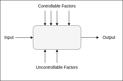
The goal of an experiment is to find the best configuration of controllable factors that maximizes the response function while minimizing the impact of uncontrollable factors. A well-designed experiment needs two key elements: a systematic way to test different combinations of controllable factors, and a method to account for randomness from uncontrollable factors.
Building on these principles, a clear and organized framework is crucial for effectively designing and conducting experiments. Below, we present a checklist that guides a practitioner through the planning and execution of an ML experiment.
To plan and perform a rigorous ML experiment:
The objective should state clearly why is the experiment to be performed. It is also important to specify a meaningful effect size. For example, if the goal of an experiment is “to determine the if using a data augmentation technique improves my model’s accuracy”, then we must add, “a significant improvement is greater than or equal to 5%.”
The response function of a Machine Learning experiment is typically an accuracy metric relative to the task of the learning function, such as classification accuracy, mean average precision, or mean squared error. It could also be a measure of interpretability, robustness or complexity — so long as the metric is be well-defined.
A machine learning system has several controllable factors, such as model design, data pre-processing, training strategy, and feature selection. In this step, we decide what factors remain static, and what can vary across runs. For example, if the objective is “to determine the if using a data augmentation technique improves my model’s accuracy”, we could choose to vary the data augmentation strategies and their parameters, but keep the model the same across all runs.
A run is a single instance of the experiment, where a process is applied to a single configuration of factors. In our example experiment with the aim “to determine the if using a data augmentation technique improves my model’s accuracy”, a single run would be: “to train a model on a training dataset using one data augmentation technique and measure its accuracy on a held-out test set.”
In this step, we also select the data for our experiment. When choosing datasets, we must consider whether our experiment a domain-specific application or for generic use. A domain-specific experiment typically requires a single dataset that is representative of the domain, while experiments that aim to show a generic result should evaluate methods across multiple datasets with diverse data types [1].
In both cases, we must define specifically the training, validation and testing datasets. If we are splitting one dataset, we should record the data splits. This is an essential step in avoiding accidental contamination!
The experimental design is is the collection of runs that we will perform. An experiment design describes:
If we are running an experiment to test the impact of training dataset size on the resulting model’s robustness, which range of sizes will we test, and how granular should we get? When varying multiple factors, does it make sense to test all possible combinations of all factor/level configurations? If we plan to perform statistical tests, it could be helpful to follow a specific experiment design, such as a factorial design or randomized block design (see [3] for more information).
Cross validation is essential for ML experiments, as this reduces the variance of your results which come from the choice of dataset split. To determine the number of cross-validation samples needed, we return to our objective statement in Step 1. If we plan to perform a statistical analysis, we need to ensure that we generate enough data for our specific statistical test.
A final part of this step is to think about resource constraints. How much time and compute does one run take? Do we have enough resources to run this experiment as we designed it? Perhaps the design must be altered to meet resource constraints.
To ensure that the experiment runs smoothly, It is important to have a rigorous system in place to organize data, track experiment runs, and analyze resource allocation. Several open-source tools are available for this purpose (see awesome-ml-experiment-management).
Depending on the objective and the domain of the experiment, it could suffice to look at cross-validation averages (and error bars!) of the results. However, the best way to validate results is through statistical hypothesis testing, which rigorously shows that the probability of obtaining your results given the data is not due to chance. Statistical testing is necessary if the objective of the experiment is to show a cause-and-effect relationship.
Depending on the analysis in the previous step, we can now state the conclusions we draw from our experiment. Can we make any claims from our results, or do we need to see more data? Solid conclusions are backed by the resulting data and are reproducible. Any practitioner who is unfamiliar with the experiment should be able to run the experiment from start to finish, obtain the same results, and draw from the results the same conclusions.
A Machine Learning experiment has two key factors: a systematic design for testing different combinations of factors, and a cross-validation scheme to control for randomness. Following the ML experiment checklist of this post throughout the planning and execution of an experiment can help a practitioner, or a team of practitioners, ensure that the resulting experiments are reliable and reproducible.
Thank you for reading! If you found this post useful, please consider following me on Medium, or checking out my website.
[1] Joris Guerin “A Quick Guide to Design Rigorous Machine Learning Experiments.” Towards Data Science. Available Online.
[2] Design & Analysis of Machine Learning Experiments — Machine Learning — Spring 2016 — Professor Kogan. YouTube video.
[3] Lawson, John. Design and analysis of experiments with R. Available Online.
[4] Questionable Practices in Machine Learning. ArXiv preprint.
[5] Improving Reproducibility in Machine Learning Research. Journal of Machine Learning Research, 2022. Available Online.
[6] A Step Toward Quantifying Independently Reproducible Machine Learning Research. ArXiv preprint.
Machine Learning Experiments Done Right was originally published in Towards Data Science on Medium, where people are continuing the conversation by highlighting and responding to this story.
Originally appeared here:
Machine Learning Experiments Done Right
Go Here to Read this Fast! Machine Learning Experiments Done Right

Originally appeared here:
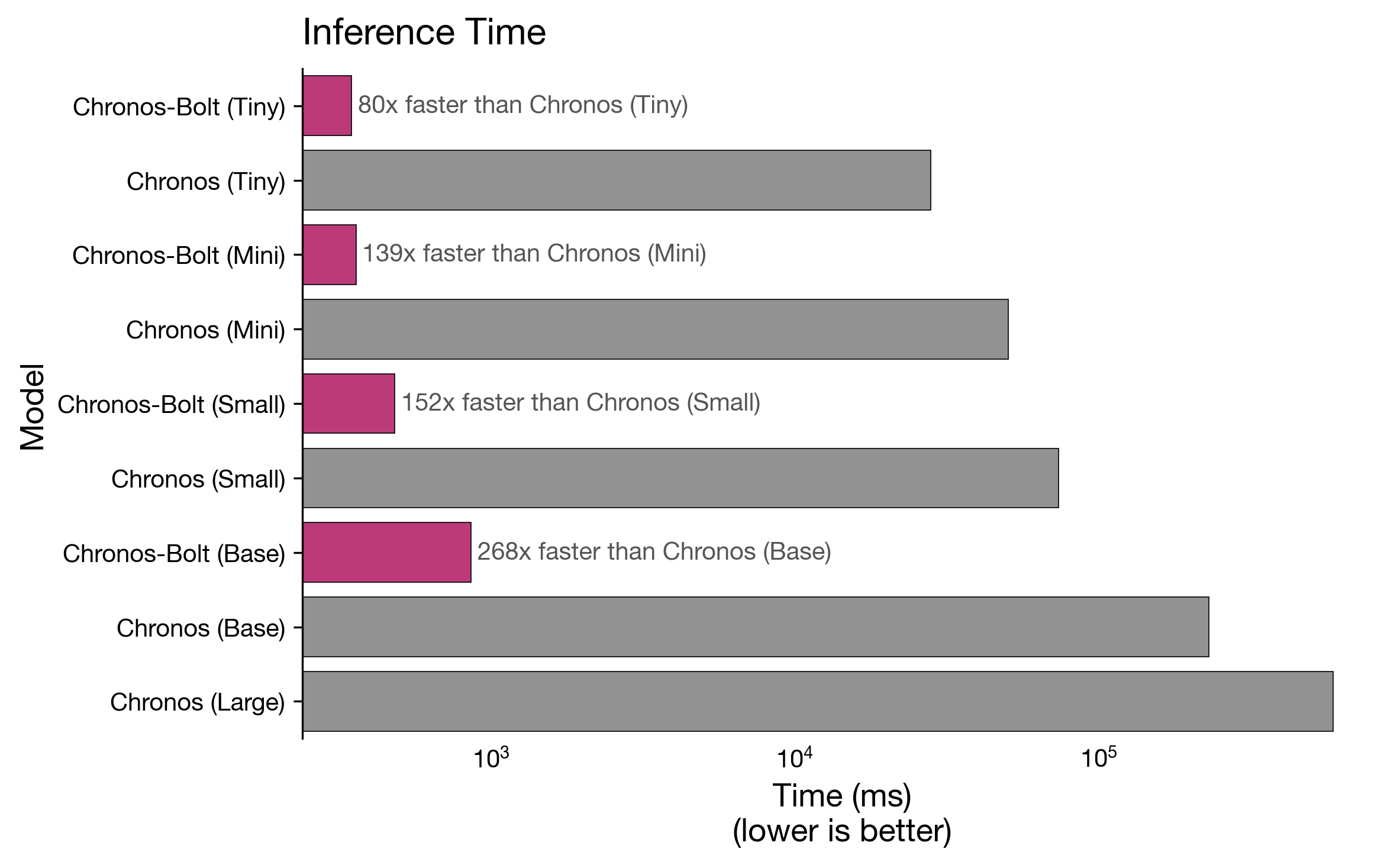
Fast and accurate zero-shot forecasting with Chronos-Bolt and AutoGluon
Go Here to Read this Fast! Fast and accurate zero-shot forecasting with Chronos-Bolt and AutoGluon


AI agents have been all the rage in 2024 and rightfully so. Unlike traditional AI models or interactions with Large Language Models (LLMs) that provide responses based on static training data, AI agents are dynamic entities that can perceive, reason (due to prompting techniques), and act autonomously within their operational domains. Their ability to adapt and optimize processes makes them invaluable in fields requiring intricate decision-making and real-time responsiveness, such as network deployment, testing, monitoring and debugging. In the coming days we will see vast adoption of AI agents across all industries, especially networking industry.
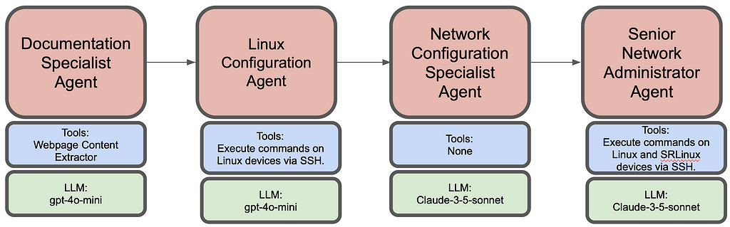
Here I demonstrate network deployment, configuration and monitoring via AI agents. Overall this agentic workflow consists of 4 agents. First one is tasked to get the installation steps from https://learn.srlinux.dev/get-started/lab/ website. Second agent executes these steps. Third agent comes up with relevant node configs based on network topology and finally the last agent executes the configuration and verifies end to end connectivity.
For details on the code playbook, please check my github link: AI-Agents-For-Networking.
For this use-case, entire topology was deployed on a pre-built Debian 12 UTM VM (as a sandbox environment). This was deliberatly chosen as it comes with all relevant packages like containerlab and docker packages pre-installed. Containerlab helps spin up various container based networking topologies with ease. Following topology was chosen which consisted of linux containers and Nokia’s SR Linux containers:
Client1 — — Leaf1 — — Spine1 — — Leaf2 — — Client2
Where Client1 and Client2 are linux containers and Leaf1 and Leaf2 are IXR-D2L and Spine1 is IXR-D5 types of SR Linux containers.
Following is the summarized workflow of each agent:
Goes over the given website url and extracts the installation steps, network topology deployment steps and finds node connection instructions. Following is the sample code to create agent, task and its custom tool:
# Custom tool to extract content from a given webpage
class QuickstartExtractor(BaseTool):
    name: str = "WebPage Content extractor"
    description: str = "Get all the content from a webpage"

    def _run(self) -> str:
            url = "https://learn.srlinux.dev/get-started/lab/"
            response = requests.get(url)
            response.raise_for_status()
            return response.text

# Create doc specialist Agent
doc_specialist = Agent(
   role="Documentation Specialist",
   goal="Extract and organize containerlab quickstart steps",
   backstory="""Expert in technical documentation with focus on clear,
   actionable installation and setup instructions.""",
   verbose=True,
   tools = [QuickstartExtractor()],
   allow_delegation=False
        )

# Task for doc speaclist Agent
doc_task = Task(
    description=(
                    "From the containerlab quickstart guide:n"
     "1. Extract installation steps n"
     "2. Identify topology deployment steps n"
     "3. Find node connection instructions n"

    "Present in a clear, sequential format.n"
    ),
                expected_output="List of commands",
    agent=doc_specialist
                )
Once run, following is an example output (Final Answer) from the agent:
# Agent: Documentation Specialist
## Final Answer:
```bash
# Installation Steps
curl -sL https://containerlab.dev/setup | sudo -E bash -s "all"

# Topology Deployment Steps
sudo containerlab deploy -c -t https://github.com/srl-labs/srlinux-getting-started

# Node Connection Instructions
ssh leaf1
```
As can be seen, it has clearly extracted the desired steps from the url. This is then passed on to the next agent.
Note: Adding code for all the agents will make this article lengthy. Kindly check my github repo for more details: AI-Agents-For-Networking.
2. Linux Configuration Agent
Executes the commands obtained from Document specialist agent. Its given the login details for UTM VM and instructed to execute the commands on that VM. It finishes by checking that all docker containers all running. It also checks the health of the VM before performing any containerlab/docker commands.
The output (Final Answer) from this agent clearly shows successful execution of VM health checks, containerlab and docker commands:
# Agent: Linux Command Executor and Docker Orchestrator
## Final Answer:
1. **System Uptime Check**:
   - Output: `14:56:17 up 1 day, 20:25, 60 users,  load average: 0.01, 0.39, 0.86`

2. **Disk Usage Check**:
   - Output:
   ```
   Filesystem                   Size  Used Avail Use% Mounted on
   udev                         5.9G     0  5.9G   0% /dev
   tmpfs                        1.2G  1.3M  1.2G   1% /run
   /dev/mapper/debian--vg-root   61G  5.7G   52G  10% /
   tmpfs                        5.9G     0  5.9G   0% /dev/shm
   tmpfs                        5.0M     0  5.0M   0% /run/lock
   /dev/sda2                    456M   92M  340M  22% /boot
   /dev/sda1                    511M  5.9M  506M   2% /boot/efi
   tmpfs                        1.2G     0  1.2G   0% /run/user/1000
   ```

3. **Running Processes Check**:
   - Output: (truncated for brevity)
   ```
   USER         PID %CPU %MEM    VSZ   RSS TTY      STAT START   TIME COMMAND
   root           1  0.0  0.1 168128 12792 ?        Ss   Nov25   1:28 /sbin/init
   ...
   debian    106849  0.0  0.0   8244  4992 pts/0    Ss+  Nov25   0:09 -bash
   ```

4. **Network Connectivity Check**:
   - Output:
   ```
   PING 8.8.8.8 (8.8.8.8) 56(84) bytes of data.
   64 bytes from 8.8.8.8: icmp_seq=1 ttl=116 time=15.4 ms
   ...
   --- 8.8.8.8 ping statistics ---
   4 packets transmitted, 4 received, 0% packet loss, time 3012ms
   rtt min/avg/max/mdev = 15.316/16.778/20.466/2.142 ms
   ```

5. **Containerlab Installation Check**:
   - Containerlab is already installed and is at the latest version (0.59.0).

6. **Topology Deployment Output**:
   - Output of the deployed topology:
   ```
   +---+---------+--------------+------------------------------------+---------------+---------+----------------+----------------------+
   | # |  Name   | Container ID |               Image                |     Kind      |  State  |  IPv4 Address  |     IPv6 Address     |
   +---+---------+--------------+------------------------------------+---------------+---------+----------------+----------------------+
   | 1 | client1 | ab894528a0e9 | ghcr.io/srl-labs/network-multitool | linux         | running | 172.20.20.4/24 | 3fff:172:20:20::4/64 |
   | 2 | client2 | 6f9f0822be5d | ghcr.io/srl-labs/network-multitool | linux         | running | 172.20.20.2/24 | 3fff:172:20:20::2/64 |
   | 3 | leaf1   | e7a1a3874600 | ghcr.io/nokia/srlinux:24.7.2       | nokia_srlinux | running | 172.20.20.3/24 | 3fff:172:20:20::3/64 |
   | 4 | leaf2   | ed4399b8f7d6 | ghcr.io/nokia/srlinux:24.7.2       | nokia_srlinux | running | 172.20.20.5/24 | 3fff:172:20:20::5/64 |
   | 5 | spine1  | ada601805590 | ghcr.io/nokia/srlinux:24.7.2       | nokia_srlinux | running | 172.20.20.6/24 | 3fff:172:20:20::6/64 |
   +---+---------+--------------+------------------------------------+---------------+---------+----------------+----------------------+
   ```

7. **List of Running Docker Containers**:
   - Output:
   ```
   CONTAINER ID   IMAGE                                COMMAND                  CREATED         STATUS         PORTS                                          NAMES
   ada601805590   ghcr.io/nokia/srlinux:24.7.2         "/tini -- fixuid -q …"   4 minutes ago   Up 4 minutes                                                  spine1
   6f9f0822be5d   ghcr.io/srl-labs/network-multitool   "/bin/sh /docker/ent…"   4 minutes ago   Up 4 minutes   22/tcp, 80/tcp, 443/tcp, 1180/tcp, 11443/tcp   client2
   e7a1a3874600   ghcr.io/nokia/srl-labs/network-multitool   "/bin/sh /docker/ent…"   4 minutes ago   Up 4 minutes                                                  leaf1
   ab894528a0e9   ghcr.io/nokia/srl-labs/network-multitool   "/bin/sh /docker/ent…"   4 minutes ago   Up 4 minutes                                                  client1
   ed4399b8f7d6   ghcr.io/nokia/srlinux:24.7.2         "/tini -- fixuid -q …"   4 minutes ago   Up 4 minutes                                                  leaf2
   ```

All tasks completed successfully with the appropriate outputs!
3. Network Configuration Specialist Agent
The job of this agent is to understand the topology i.e. the number of nodes and their connectivity. It then needs to come up with ip allocation scheme, generate relevant interface and routing configuration of linux containers and SR Linux containers alongwith adhering to the ip allocation scheme.
For SR Linux configuration an example config was given in the prompt. This example config could have also been obtained from a configuration guide in pdf format which would have been RAGed by the agent (given the right tools).
In the output of this agent below, it can clearly be seen that it has succesfully come up with ip allocation based on the topology, the relevant configurations and routes:
# Agent: Senior Network Administrator
## Final Answer:
# Configuration for client1 (Linux)
```bash
/sbin/ip address add 10.1.1.2/24 dev eth1
/sbin/ip route add 10.1.4.2/32 via 10.1.1.1
```

# Configuration for leaf1 (SRLinux)
```bash
enter candidate private
# configure data interfaces
set / interface ethernet-1/1 admin-state enable
set / interface ethernet-1/1 subinterface 0 admin-state enable
set / interface ethernet-1/1 subinterface 0 ipv4 address 10.1.1.1/24
set / interface ethernet-1/1 subinterface 0 ipv4 admin-state enable
set / interface ethernet-1/49 admin-state enable
set / interface ethernet-1/49 subinterface 0 admin-state enable
set / interface ethernet-1/49 subinterface 0 ipv4 address 10.1.2.1/24
set / interface ethernet-1/49 subinterface 0 ipv4 admin-state enable
# add interfaces to default namespace
set / network-instance default interface ethernet-1/1.0
set / network-instance default interface ethernet-1/49.0
# configure BGP
set / network-instance default protocols bgp admin-state enable
set / network-instance default protocols bgp router-id 1.1.1.1
set / network-instance default protocols bgp autonomous-system 65001
set / network-instance default protocols bgp afi-safi ipv4-unicast admin-state enable
set / network-instance default protocols bgp group ebgp admin-state enable
set / network-instance default protocols bgp group ebgp export-policy [ export-all ]
set / network-instance default protocols bgp group ebgp import-policy [ export-all ]
set / network-instance default protocols bgp neighbor 10.1.2.2 admin-state enable
set / network-instance default protocols bgp neighbor 10.1.2.2 peer-group ebgp
set / network-instance default protocols bgp neighbor 10.1.2.2 peer-as 65002
# create policy
set / routing-policy policy export-all default-action policy-result accept
commit now
```

# Configuration for spine1 (SRLinux)
```bash
enter candidate private
# configure data interfaces
set / interface ethernet-1/1 admin-state enable
set / interface ethernet-1/1 subinterface 0 admin-state enable
set / interface ethernet-1/1 subinterface 0 ipv4 address 10.1.2.2/24
set / interface ethernet-1/1 subinterface 0 ipv4 admin-state enable
set / interface ethernet-1/2 admin-state enable
set / interface ethernet-1/2 subinterface 0 admin-state enable
set / interface ethernet-1/2 subinterface 0 ipv4 address 10.1.3.1/24
set / interface ethernet-1/2 subinterface 0 ipv4 admin-state enable
# add interfaces to default namespace
set / network-instance default interface ethernet-1/1.0
set / network-instance default interface ethernet-1/2.0
# configure BGP
set / network-instance default protocols bgp admin-state enable
set / network-instance default protocols bgp router-id 2.2.2.2
set / network-instance default protocols bgp autonomous-system 65002
set / network-instance default protocols bgp afi-safi ipv4-unicast admin-state enable
set / network-instance default protocols bgp group ebgp admin-state enable
set / network-instance default protocols bgp group ebgp export-policy [ export-all ]
set / network-instance default protocols bgp group ebgp import-policy [ export-all ]
set / network-instance default protocols bgp neighbor 10.1.2.1 admin-state enable
set / network-instance default protocols bgp neighbor 10.1.2.1 peer-group ebgp
set / network-instance default protocols bgp neighbor 10.1.2.1 peer-as 65001
set / network-instance default protocols bgp neighbor 10.1.3.2 admin-state enable
set / network-instance default protocols bgp neighbor 10.1.3.2 peer-group ebgp
set / network-instance default protocols bgp neighbor 10.1.3.2 peer-as 65003
# create policy
set / routing-policy policy export-all default-action policy-result accept
commit now
```

# Configuration for leaf2 (SRLinux)
```bash
enter candidate private
# configure data interfaces
set / interface ethernet-1/1 admin-state enable
set / interface ethernet-1/1 subinterface 0 admin-state enable
set / interface ethernet-1/1 subinterface 0 ipv4 address 10.1.4.1/24
set / interface ethernet-1/1 subinterface 0 ipv4 admin-state enable
set / interface ethernet-1/49 admin-state enable
set / interface ethernet-1/49 subinterface 0 admin-state enable
set / interface ethernet-1/49 subinterface 0 ipv4 address 10.1.3.2/24
set / interface ethernet-1/49 subinterface 0 ipv4 admin-state enable
# add interfaces to default namespace
set / network-instance default interface ethernet-1/1.0
set / network-instance default interface ethernet-1/49.0
# configure BGP
set / network-instance default protocols bgp admin-state enable
set / network-instance default protocols bgp router-id 3.3.3.3
set / network-instance default protocols bgp autonomous-system 65003
set / network-instance default protocols bgp afi-safi ipv4-unicast admin-state enable
set / network-instance default protocols bgp group ebgp admin-state enable
set / network-instance default protocols bgp group ebgp export-policy [ export-all ]
set / network-instance default protocols bgp group ebgp import-policy [ export-all ]
set / network-instance default protocols bgp neighbor 10.1.3.1 admin-state enable
set / network-instance default protocols bgp neighbor 10.1.3.1 peer-group ebgp
set / network-instance default protocols bgp neighbor 10.1.3.1 peer-as 65002
# create policy
set / routing-policy policy export-all default-action policy-result accept
commit now
```

# Configuration for client2 (Linux)
```bash
/sbin/ip address add 10.1.4.2/24 dev eth1
/sbin/ip route add 10.1.1.2/32 via 10.1.4.1
```

This configuration:
1. Uses unique subnets for each connection:
   - client1-leaf1: 10.1.1.0/24
   - leaf1-spine1: 10.1.2.0/24
   - spine1-leaf2: 10.1.3.0/24
   - leaf2-client2: 10.1.4.0/24

2. Configures BGP with unique AS numbers:
   - leaf1: AS65001
   - spine1: AS65002
   - leaf2: AS65003

3. Implements specific routes on clients for end-to-end connectivity
4. Follows the exact SRLinux configuration format provided
5. Uses proper routing policies for BGP route exchange
4. Senior Network Administrator Agent
This agent gets the configuration generated and applies it to all the nodes, checks for bgp peering to come up and then finally executes ping from end to end verifying connectivity. Here the agent gets to the right show command just by inferring from the configuration commands.
Following is the Final Answer from this agent obtained after successful configuration and of the network topology and checking end to end connectivity:
# Agent: Network Configuration Specialist
## Final Answer:
# Network Configuration Report

## Topology Information
### Devices and Interfaces
1. **client1**
   - Interface: eth1
   - IP: 10.1.1.2/24
   - Static route: 10.1.4.2/32 via 10.1.1.1

2. **leaf1** (AS65001)
   - ethernet-1/1: 10.1.1.1/24 (connected to client1)
   - ethernet-1/49: 10.1.2.1/24 (connected to spine1)
   - BGP Router ID: 1.1.1.1

3. **spine1** (AS65002)
   - ethernet-1/1: 10.1.2.2/24 (connected to leaf1)
   - ethernet-1/2: 10.1.3.1/24 (connected to leaf2)
   - BGP Router ID: 2.2.2.2

4. **leaf2** (AS65003)
   - ethernet-1/1: 10.1.4.1/24 (connected to client2)
   - ethernet-1/49: 10.1.3.2/24 (connected to spine1)
   - BGP Router ID: 3.3.3.3

5. **client2**
   - Interface: eth1
   - IP: 10.1.4.2/24
   - Static route: 10.1.1.2/32 via 10.1.4.1

## Configuration Commands Executed
All configurations were successfully applied to their respective devices as per the provided configuration scripts. The key configurations included:
1. Interface IP addressing
2. BGP neighbor relationships
3. Route policies
4. Static routes on client machines

## Connectivity Test Results
```
PING 10.1.4.2 (10.1.4.2) 56(84) bytes of data.
64 bytes from 10.1.4.2: icmp_seq=1 ttl=61 time=128 ms
64 bytes from 10.1.4.2: icmp_seq=2 ttl=61 time=8.16 ms
64 bytes from 10.1.4.2: icmp_seq=3 ttl=61 time=4.49 ms
64 bytes from 10.1.4.2: icmp_seq=4 ttl=61 time=5.86 ms

--- 10.1.4.2 ping statistics ---
4 packets transmitted, 4 received, 0% packet loss, time 3005ms
rtt min/avg/max/mdev = 4.491/36.620/127.973/52.758 ms
```

The ping test from client1 (10.1.1.2) to client2 (10.1.4.2) was successful with:
- 100% success rate (4/4 packets)
- Average round-trip time: 36.620ms
- No packet loss

This confirms that the BGP configurations are working correctly and the network is properly forwarding traffic between the clients through the leaf-spine topology.
AI agents go above and beyond automation. They can reason and try to come up with alternatives. A simple example can be if a linux command fails due to permission issue and the agent has access to sudo password, next time it will try with a sudo password to succeed. A complex example can be incase the bgp peering is not up, then based on the prompt instructions they can try to find why and even go about fixing it.
Agentic workflows have its challenges and they require different way of thinking compared to programmatic approaches. So far the downsides that I have encountered include that it can take longer (sometimes way longer) to achieve an outcome, runtimes vary with each run and outputs can vary (this can somewhat be controlled by better prompts).
Finally, for trivial, straightforward tasks like scraping a website and executing the given set of commands, a smaller LLM can be used like gpt-4o-mini or llama3.1–7b etc. However, for tasks like designing the network topology, a bigger LLM is required. Although here claude-3–5-sonnet was chosen but ideally a good 70b model should suffice. Finally, you have to be very diligent with prompts. They will make or break your use-case!
AI Agents in Networking Industry was originally published in Towards Data Science on Medium, where people are continuing the conversation by highlighting and responding to this story.
Originally appeared here:
AI Agents in Networking Industry

The second season of Arcane, a recent blockbuster series on Netflix based on the universe of one of the most popular online video games ever, League of Legends, is set in a fantasy world with heavy steampunk design, closed with astonishing visuals and a record-breaking budget. As a good network and data scientist with a particular interest in turning pop cultural items into data visualization, this was all I needed after finishing the closing season to map out the hidden connections and turn the storyline of Arcane into a network visualization — using Python. Hence, by the end of this tutorial, you will have hands-on skills on how to create and visualize the network behind Arcane.
However, these skills and methods are absolutely not specific to this story. In fact, they highlight the general approach network science provides to map out, design, visualize, and interpret networks of any complex system. These systems can range from transportation and COVID-19 spreading network patterns to brain networks to various social networks, such as that of the Arcane series.
All images created by the author.
Since here we are going to map out the connections behind all characters, first, we need to get a list of each character. For this, the Arcane fan wiki site is an excellent source of free-to-use information (CC BY-SA 3.0), which we can easily access by simple web scraping techniques. Namely, we will use urllib to download, and with BeautifulSoup, we will extract the names and fan wiki profile URLs of each character listed on the main character page.
First downloading the character listing site’s html:
import urllib
import bs4 as bs
from urllib.request import urlopen


url_char = 'https://arcane.fandom.com/wiki/Category:Characters'

sauce = urlopen(url_char).read()
soup  = bs.BeautifulSoup(sauce,'lxml')
Then, I extracted all the potentially relevant names. One can easily figure out what tags to feed the parsed html stored in the ‘soup’ variable by just right-clicking on a desired element (in this case, a character profile) and selecting the element inspection option in any browser.
From this, I learned that the name and url of a character are stored in a line which has ‘title=’ in it, but does not contain ‘:’ (which corresponds to categories). Additionally, I created a still_character flag, which helped me decide which subpages on the character listing page still belong to legitimate characters of the story.
import re

chars = soup.find_all('li')
still_character = True
names_urls = {}

for char in chars:

    if '" title="' in str(char) and ':' not in char.text and still_character:

        char_name = char.text.strip().rstrip()

        if char_name == 'Arcane':
            still_character = False

        char_url = 'https://arcane.fandom.com' + re.search(r'href="([^"]+)"', str(char)).group(1)

        if still_character:
            names_urls[char_name] = char_url
The previous code block will create a dictionary (‘names_urls’) which stores the name and url of each character as key-value pairs. Now let’s have a quick look at what we have and print the name-url dictionary and the total length of it:
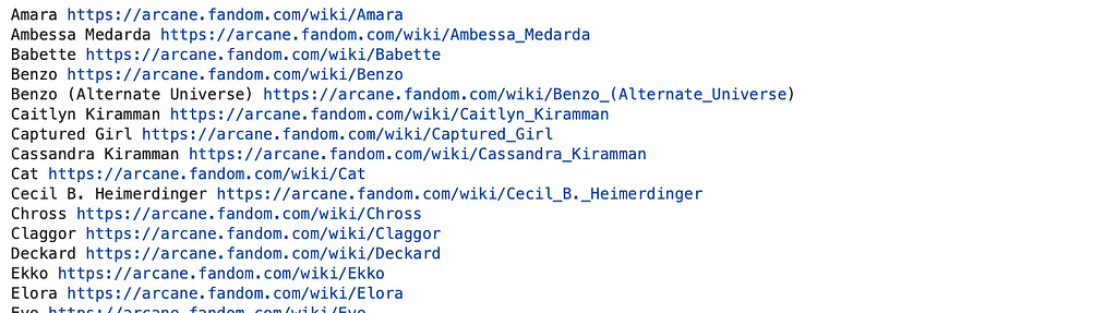
for name, url in names_urls.items():
    print(name, url)
A sample of the output from this code block, where we can text each link — pointing to the biography profile of each character:
print(len(names_urls))
Which code cell returns the result of 67, implying the total number of named characters we have to deal with. This means we are already done with the first task — we have a comprehensive list of characters as well as easy access to their full textual profile on their fan wiki sites.
To map out the connections between two characters, we figure out a way to quantify the relationship between each two characters. To capture this, I rely on how frequently the two character’s biographies reference each other. On the technical end, to achieve this, we will need to collect these complete biographies we just got the links to. We will get that again using simple web scraping techniques, and then save the source of each site in a separate file locally as follows.
# output folder for the profile htmls
import os
folderout = 'fandom_profiles'
if not os.path.exists(folderout):
    os.makedirs(folderout)

# crawl and save the profile htmls
for ind, (name, url) in enumerate(names_urls.items()):
    if not os.path.exists(folderout + '/' + name + '.html'):
        fout = open(folderout + '/' + name + '.html', "w")
        fout.write(str(urlopen(url).read()))
        fout.close()
By the end of this section, our folder ‘fandom_profiles’ should contain the fanwiki profiles of each Arcane character — ready to be processed as we work our way towards building the Arcane network.
To build the network between characters, we assume that the intensity of interactions between two characters is signaled by the number of times each character’s profile mentions the other. Hence, the nodes of this network are the characters, which are linked with connections of varying strength based on the number of times each character’s wiki site source references any other character’s wiki.
In the following code block, we build up the edge list — the list of connections that contains both the source and the target node (character) of each connection, as well as the weight (co-reference frequency) between the two characters. Additionally, to conduct the in-profile search effectively, I create a names_ids which only contains the specific identifier of each character, without the rest of the web address.
# extract the name mentions from the html sources
# and build the list of edges in a dictionary
edges = {}
names_ids  = {n : u.split('/')[-1] for n, u in names_urls.items()}

for fn in [fn for fn in os.listdir(folderout) if '.html' in fn]:

    name = fn.split('.html')[0]

    with open(folderout + '/' + fn) as myfile:
        text = myfile.read()
        soup  = bs.BeautifulSoup(text,'lxml')
        text = ' '.join([str(a) for a in soup.find_all('p')[2:]])
        soup = bs.BeautifulSoup(text,'lxml')


        for n, i in names_ids.items():

            w = text.split('Image Gallery')[0].count('/' + i)
            if w>0:
                edge = 't'.join(sorted([name, n]))
                if edge not in edges:
                    edges[edge] = w
                else:
                    edges[edge] += w

len(edges)
As this code block runs, it should return around 180 edges.
Next, we use the NetworkX graph analytics library to turn the edge list into a graph object and output the number of nodes and edges the graph has:
#  create the networkx graph from the dict of edges
import networkx as nx
G = nx.Graph()
for e, w in edges.items():
    if w>0:
        e1, e2 = e.split('t')
        G.add_edge(e1, e2, weight=w)

G.remove_edges_from(nx.selfloop_edges(G))

print('Number of nodes: ', G.number_of_nodes())
print('Number of edges: ', G.number_of_edges())
The output of this code block:
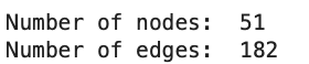
This output tells us that while we started with 67 characters, 16 of them ended up not being connected to anyone in the network, hence the smaller number of nodes in the constructed graph.
Once we have the network, we can visualize it! First, let’s create a simple draft visualization of the network using Matplotlib and the built-in tools of NetworkX.
# take a very brief look at the network
import matplotlib.pyplot as plt
f, ax = plt.subplots(1,1,figsize=(15,15))
nx.draw(G, ax=ax, with_labels=True)
plt.savefig('test.png')
The output image of this cell:
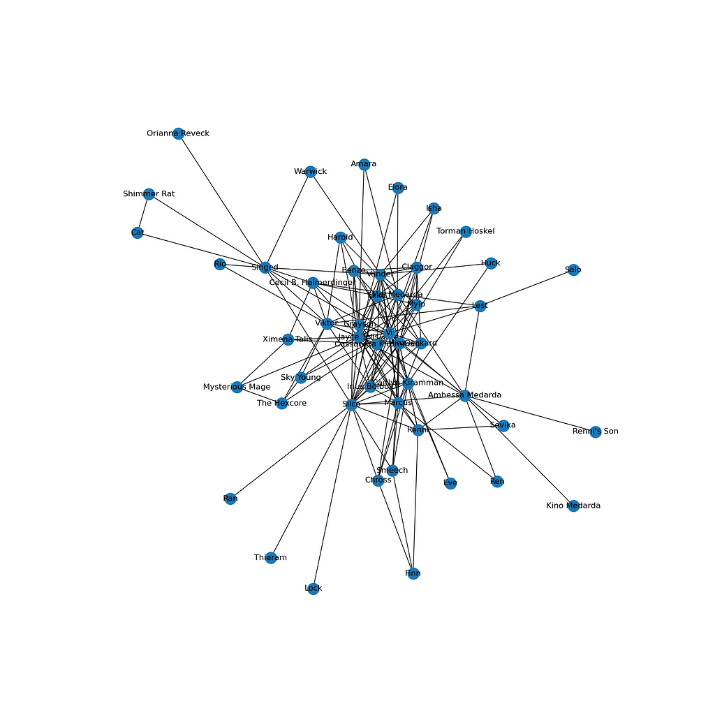
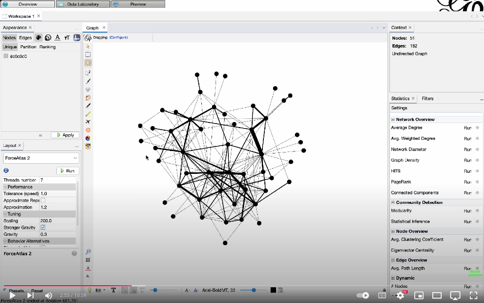
While this network already gives a few hints about the main structure and most frequent characteristics of the show, we can design a much more detailed visualization using the open-source network visualization software Gephi. For this, we need to export the network into a .gexf graph data file first, as follows.
nx.write_gexf(G, 'arcane_network.gexf')
Now, the tutorial on how to visualize this network using Gephi:
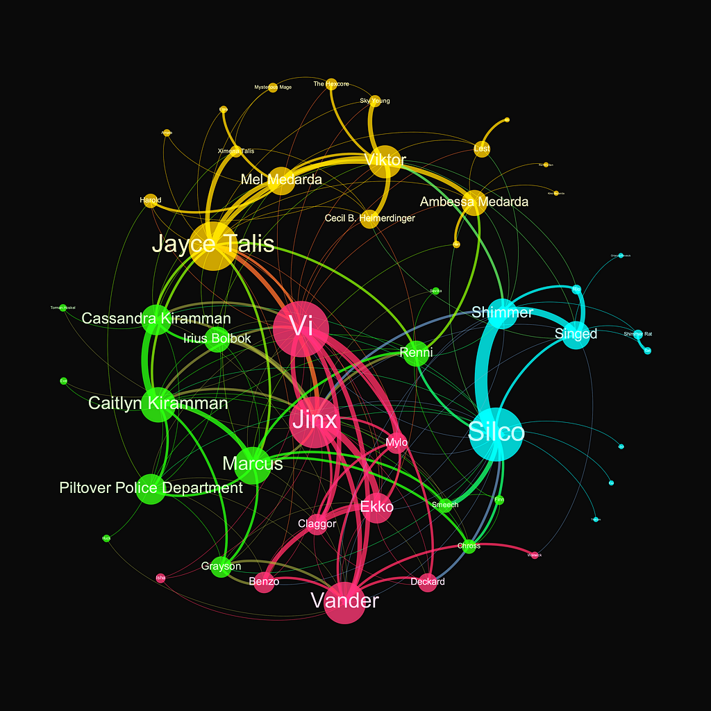
Here comes an extension part, which I am referring to in the video. After exporting the node table, including the network community indices, I read that table using Pandas and assigned individual colors to each community. I got the colors (and their hex codes) from ChatGPT, asking it to align with the main color themes of the show. Then, this block of code exports the color—which I again used in Gephi to color the final graph.
import pandas as pd
nodes = pd.read_csv('nodes.csv')

pink = '#FF4081'
blue = '#00FFFF'
gold = '#FFD700'
silver = '#C0C0C0'
green = '#39FF14'

cmap = {0 : green,
        1 : pink,
        2 : gold,
        3 : blue,
    }

nodes['color'] = nodes.modularity_class.map(cmap)
nodes.set_index('Id')[['color']].to_csv('arcane_colors.csv')
As we color the network based on the communities we found (communities meaning highly interconnected subgraphs of the original network), we uncovered four major groups, each corresponding to specific sets of characters within the storyline. Not so surprisingly, the algorithm clustered together the main protagonist family with Jinx, Vi, and Vander (pink). Then, we also see the cluster of the underground figures of Zaun (blue), such as Silco, while the elite of Piltover (blue) and the militarist enforce (green) are also well-grouped together.
The beauty and use of such community structures is that while such explanations put it in context very easily, usually, it would be very hard to come up with a similar map only based on intuition. While the methodology presented here clearly shows how we can use network science to extract the hidden connections of virtual (or real) social systems, let it be the partners of a law firm, the co-workers of an accounting firm, and the HR department of a major oil company.
The Arcane Network was originally published in Towards Data Science on Medium, where people are continuing the conversation by highlighting and responding to this story.
Originally appeared here:
The Arcane Network


Using visualization to understand the relationship between two variables
Originally appeared here:
Visualizing Regression Models with Seaborn
Go Here to Read this Fast! Visualizing Regression Models with Seaborn

Originally appeared here:
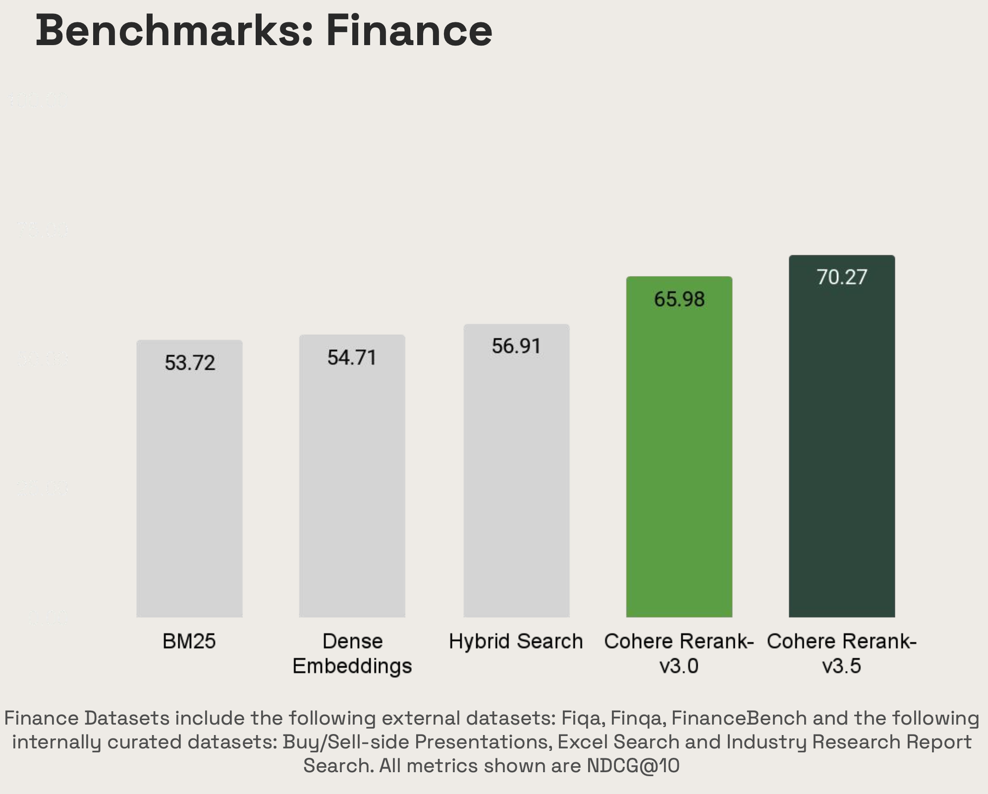
Cohere Rerank 3.5 is now available in Amazon Bedrock through Rerank API
Go Here to Read this Fast! Cohere Rerank 3.5 is now available in Amazon Bedrock through Rerank API