Category: AI

  • Fraud Detection with Generative Adversarial Nets (GANs)

    Michio Suginoo

    Application of GANs for data augmentation to adjust an imbalanced dataset

    Photo by Brett Jordan on Unsplash

    “Generative Adversarial Nets” (GANs) demonstrated outstanding performance in generating realistic synthetic data which are indistinguishable from the real data in the past. Unfortunately, GANs caught the public’s attention because of its unethical applications, deepfakes (Knight, 2018).

    This article illustrates a case with a good motive in the application of GANs in the context of fraud detection.

    Fraud detection is an application of binary classification prediction. Fraud cases, which account for only a small fraction of the transaction universe, constitute a minority class that makes the dataset highly imbalanced. In general, the resulting model tends to be biased towards the majority class and tends to underfit to the minority class. Thus, the less balanced the dataset, the poorer the performance of the classification predictor would be.

    My motive here is to use GANs as a data augmentation tool in an attempt to address this classical problem of fraud detection associated with the imbalanced dataset. More specifically, GANs can generate realistic synthetic data of the minority fraud class and transform the imbalanced dataset perfectly balanced.

    And, I am hoping that this sophisticated algorithm could materially contribute to the performance of fraud detection. In other words, my initial expectation is: the better sophisticated algorithm, the better performance.

    A relevant question is if the use of GANs will guarantee a promising improvement in the performance of fraud detection and satisfy my motive. Let’s see.

    Introduction

    In principle, fraud detection is an application of binary classification algorithm: to classify each transaction whether it is a fraud case or not.

    Fraud cases account for only a small fraction of the transaction universe. In general, fraud cases constitute the minority class, thus, make the dataset highly imbalanced.

    The fewer fraud cases, the more sound the transaction system would be.

    Very simple and intuitive.

    Paradoxically, that sound condition was one of the primary reasons that made fraud detection challenging in the past, if not impossible. It is simply because it was difficult for a classification algorithm to learn the probability distribution of the minority class of fraud.

    In general, the more balanced the dataset, the better the performance of the classification predictor. In other words, the less balanced (or the more imbalanced) the dataset, the poorer the performance of classifier.

    This paints the classical problem of fraud detection: a binary classification application with highly imbalanced dataset.

    In this setting, we can use Generative Adversarial Nets (GANs) as a data augmentation tool to generate realistic synthetic data of the minority fraud class to transform the entire dataset more balanced in an attempt to improve the performance of the classifier model of fraud detection.

    This article is divided into the following sections:

    • Section 1: Algorithm Overview: Bi-level Optimization Architecture of GANs
    • Section 2: Fraud Dataset
    • Section 3: Python Code breakdown of GANs for data augmentation
    • Section 4: Fraud Detection Overview (Benchmark Scenario vs GANs Scenario)
    • Section 5: Conclusion

    Overall, I will primarily focus on the topic of GANs (both the algorithm and the code). For the remaining topics of the model development other than GANs, such as data preprocessing and classifier algorithm, I will only outline the process and refrain from going into their details. In this context, this article assumes that the readers have a basic knowledge about the binary classifier algorithm (especially, Ensemble Classifier that I selected for fraud detection) as well as general understanding of data cleaning and preprocessing.

    For the detailed code, the readers are welcome to access the following link: https://github.com/deeporigami/Portfolio/blob/6538fcaad1bf58c5f63d6320ca477fa867edb1df/GAN_FraudDetection_Medium_2.ipynb

    Section 1: Algorithm Overview: Bi-level Optimization Architecture of GANs

    GANs is a special type of generative algorithm. As its name suggests, Generative Adversarial Nets (GANs) is composed of two neural networks: the generative network (the generator) and the adversarial network (the discriminator). GANs pits these two agents against each other to engage in a competition, where the generator attempts to generate realistic synthetic data and the discriminator to distinguish the synthetic data from the real data.

    The original GANs was introduced in a seminal paper: “Generative Adversarial Nets” (Goodfellow, et al., Generative Adversarial Nets, 2014). The co-authors of the original GANs portrayed GANs with a counterfeiter-police analogy: an iterative game, where the generator acts as a counterfeiter and the discriminator plays the role of the police to detect the counterfeit that the generator forged.

    The original GANs was innovative in a sense that it addressed and overcame conventional difficulties in training deep generative algorithm in the past. And as its core, it was designed with bi-level optimization framework with an equilibrium seeking objective setting (vs maximum likelihood oriented objective setting).

    Ever since, many variant architectures of GANs have been explored. As a precaution, this article refers solely to the prototype architecture of the original GANs.

    Generator and Discriminator

    Repeatedly, in the architecture of GANs, the two neural networks — the generator and the discriminator — compete against each other. In this context, the competition takes place through the iteration of forward propagation and backward propagation (according to the general framework of neural networks).

    On one hand, it is straight-forward that the discriminator is a binary classifier by design: it classifies whether each sample is real (label: 1) or fake/synthetic (label:0). And the discriminator is fed with both the real samples and the synthetic samples during the forward propagation. Then, during the backpropagation, it learns to detect the synthetic data from the mixed data feed.

    On the other hand, the generator is a noise distribution by design. The generator is fed with the real samples during the forward propagation. Then, during the backward propagation, the generator learns the probability distribution of the real data in order to better simulate its synthetic samples.

    And these two agents are trained alternately via “bi-level optimization” framework.

    Bi-level Training Mechanism (bi-level optimization method)

    In the original GAN paper, in order to train these two agents that pursue their diametrically opposite objectives, the co-authors designed a “bi-level optimization (training)” architecture, in which one internal training block (training of the discriminator) is nested within another high-level training block (training of the generator).

    The image below illustrates the structure of “bi-level optimization” in the nested training loops. The discriminator is trained within the nested inner loop, while the generator is trained in the main loop at the higher level.
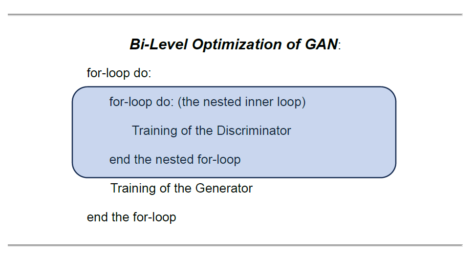
    Image by Author

    And GANs trains these two agents alternately in this bi-level training architecture (Goodfellow, et al., Generative Adversarial Nets, 2014, p. 3). In other words, while training one agent during the alternation, we need to freeze the learning process of the other agent (Goodfellow I. , 2015, p. 3).

    Mini-Max Optimization Objective

    In addition to the “bi-level optimization” mechanism which enables the alternate training of these two agents, another unique feature that differentiates GANs from the conventional prototype of neural network is its mini-max optimization objective. Simply put, in contrast to the conventional maximum seeking approach (such as maximum-likelihood) , GANs pursues an equilibrium-seeking optimization objective.

    What is an equilibrium-seeking optimization objective?

    Let’s break it down.

    GANs’ two agents have two diametrically opposite objectives. While the discriminator, as a binary classifier, aims at maximizing the probability of correctly classifying the mixture of the real samples and the synthetic samples, the generator’s objective is to minimize the probability that the discriminator correctly classifies the synthetic data: simply because the generator needs to fool the discriminator.

    In this context, the co-authors of the original GANs called the overall objective a “minimax game”. (Goodfellow, et al., 2014, p. 3)

    Overall, the ultimate mini-max optimization objective of GANs is not to search for the global maximum/minimum of either of these objective functions. Instead, it is set to seek an equilibrium point which can be interpreted as:

    • “a saddle point that is a local maximum for the classifier and a local minimum for the generator” (Goodfellow I. , 2015, p. 2)
    • where neither of agents can improve their performance any longer.
    • where the synthetic data that the generator learned to create has become realistic enough to fool the discriminator.

    And the equilibrium point could be conceptually represented by the probability of random guessing, 0.5 (50%), for the discriminator: D(z) => 0.5 .

    Let’s transcribe the conceptual framework of GANs’ minimax optimization in terms of their objective functions.

    The objective of the discriminator is to maximize the objective function in the following image:

    Image by Author

    In order to resolve a potential saturation issue, they converted the second term of the original log-likelihood objective function for the generator as follows and recommended to maximize the converted version as the generator’s objective:

    Image by Author

    Overall, the architecture of GANs’ “bi-level optimization” can be translated in to the following algorithm.

    Image by Author

    For more details about the algorithmic design of GANs, please read another article of mine: Mini-Max Optimization Design of Generative Adversarial Nets .

    Now, let’s move on to the actual coding with a dataset.

    In order to highlight GANs algorithm, I will primarily focus on the code of GANs here and only outline the rest of the process.

    Section 2: Fraud Dataset

    For fraud detection, I selected the following dataset of credit card transactions from Kaggle: https://www.kaggle.com/datasets/mlg-ulb/creditcardfraud

    Data License: Database Contents License (DbCL) v1.0

    Here is a summary of the dataset.

    The dataset contains 284,807 transactions. In the dataset, we have only 492 fraud cases (including 29 duplicated cases).

    Since the fraud class accounts for only 0.172% of all transactions, it constitutes an extremely small minority class. This dataset is an appropriate one for illustrating the classical problem of fraud detection associated with the imbalanced dataset.

    It has the following 30 features:

    • V1, V2, … V28: 28 principal components obtained by PCA. The source of the data is not disclosed for the privacy protection purpose.
    • ‘Time’: the seconds elapsed between each transaction and the first transaction of the dataset.
    • ‘Amount’: the amount of the transaction.

    The label is set as ‘Class’.

    • ‘Class’: 1 in case of fraud; and 0 otherwise.

    Data Preprocessing: Feature Selection

    Since the dataset has already been pretty much, if not perfectly, cleaned, I only had to do few things for the data cleaning: elimination of duplicated data and removal of outliers.

    Thereafter, given 30 features in the dataset, I decided to run the feature selection to reduce the number of the features by eliminating less important features before the training process. I selected the built-in feature importance score of the scikit-learn Random Forest Classifier to estimate the scores of all the 30 features.

    The following chart displays the summary of the result. If interested in the detailed process, please visit my code listed above.
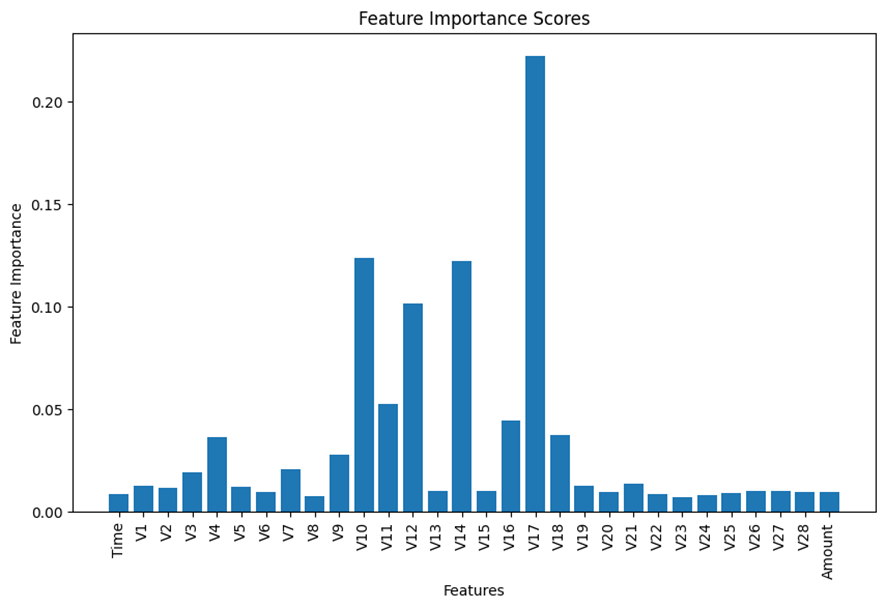
    Image by Author

    Based on the results displayed in the bar chart above, I made my subjective judgement to select the top 6 features for the analysis and remove all the remaining insignificant features from the model building process.

    Here is the selected top 6 important features.
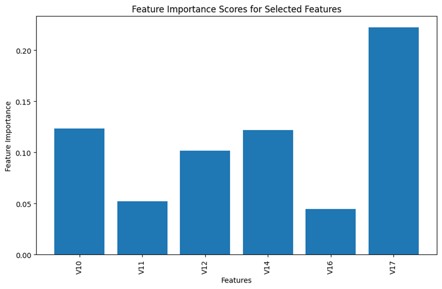
    Image by Author

    For the model building purpose going forward, I focused on these 6 selected features. After the data preprocessing, we have the working dataframe, df, of the following shape:

    • df.shape = (282513, 7)

    Hopefully, the feature selection would reduce the complexity of the resulting model and stabilize its performance, while retaining critical information for optimizing a binary classifier.

    Scenario 3: Code breakdown of GANs for data augmentation

    Finally, it’s time for us to use GANs for data augmentation.

    So how many synthetic data do we need to create?

    First of all, our interest for the data augmentation is only for the model training. Since the test dataset is out-of-sample data, we want to preserve the original form of the test dataset. Secondly, because our intention is to transform the imbalanced dataset perfectly, we do not want to augment the majority class of non-fraud cases.

    Simply put, we want to augment only the train dataset of the minority fraud class, nothing else.

    Now, let’s split the working dataframe into the train dataset and the test dataset in 80/20 ratio, using a stratified data split method.

    # Separate features and target variable
    X = df.drop('Class', axis=1)
    y = df['Class']

    # Splitting data into train and test sets
    X_train, X_test, y_train, y_test = train_test_split(X, y, test_size=0.2, random_state=42, stratify=y)

    # Combine the features and the label for the train dataset
    train_df = pd.concat([X_train, y_train], axis=1)

    As a result, the shape of the train dataset is as follows:

    • train_df.shape = (226010, 7)

    Let’s see the composition (the fraud cases and the non-fraud cases) of the train dataset.

    # Load the dataset (fraud and non-fraud data)
    fraud_data = train_df[train_df['Class'] == 1].drop('Class', axis=1).values
    non_fraud_data = train_df[train_df['Class'] == 0].drop('Class', axis=1).values

    # Calculate the number of synthetic fraud samples to generate
    num_real_fraud = len(fraud_data)
    num_synthetic_samples = len(non_fraud_data) - num_real_fraud
    print("# of non-fraud: ", len(non_fraud_data))
    print("# of Real Fraud:", num_real_fraud)
    print("# of Synthetic Fraud required:", num_synthetic_samples)

    # of non-fraud: 225632
    # of Real Fraud: 378
    # of Synthetic Fraud required: 225254

    This tells us that the train dataset (226,010) is comprised of 225,632 non-fraud data and 378 fraud data. In other words, the difference between them is 225,254. This number is the number of the synthetic fraud data (num_synthetic_samples) that we need to augment in order to perfectly match the numbers of these two classes within the train dataset: as a reminder, we do preserve the original test dataset.

    Next, let’s code GANs.

    First, let’s create custom functions to determine the two agents: the discriminator and the generator.

    For the generator, I create a noise distribution function, build_generator(), which requires two parameters: latent_dim (the dimension of the noise) as the shape of its input; and the shape of its output, output_dim, which corresponds to the number of the features.

    # Define the generator network
    def build_generator(latent_dim, output_dim):
    model = Sequential()
    model.add(Dense(64, input_shape=(latent_dim,)))
    model.add(Dense(128, activation='sigmoid'))
    model.add(Dense(output_dim, activation='sigmoid'))
    return model

    For the discriminator, I create a custom function build_discriminator() that takes input_dim, which corresponds to the number of the features.

    # Define the discriminator network
    def build_discriminator(input_dim):
    model = Sequential()
    model.add(Input(input_dim))
    model.add(Dense(128, activation='sigmoid'))
    model.add(Dense(1, activation='sigmoid'))
    return model

    Then, we can call these function to create the generator and the discriminator. Here, for the generator I arbitrarily set latent_dim to be 32: you can try other value here, if you like.

    # Dimensionality of the input noise for the generator
    latent_dim = 32

    # Build generator and discriminator models
    generator = build_generator(latent_dim, fraud_data.shape[1])
    discriminator = build_discriminator(fraud_data.shape[1])

    At this stage, we need to compile the discriminator, which is going to be nested in the main (higher) optimization loop later. And we can compile the discriminator with the following argument setting.

    • the loss function of the discriminator: the generic cross-entropy loss function for a binary classifier
    • the evaluation metrics: precision and recall.
    # Compile the discriminator model
    from keras.metrics import Precision, Recall
    discriminator.compile(optimizer=Adam(learning_rate=0.0002, beta_1=0.5), loss='binary_crossentropy', metrics=[Precision(), Recall()])

    For the generator, we will compile it when we construct the main (upper) optimization loop.

    At this stage, we can define the custom objective function for the generator as follows. Remember, the recommended objective was to maximize the following formula:

    Image by Author
    def generator_loss_log_d(y_true, y_pred):
    return - K.mean(K.log(y_pred + K.epsilon()))

    Above, the negative sign is required, since the loss function by default is designed to be minimized.

    Then, we can construct the main (upper) loop, build_GANs(generator, discriminator), of the bi-level optimization architecture. In this main loop, we compile the generator implicitly. In this context, we need to use the custom objective function of the generator, generator_loss_log_d, when we compile the main loop.

    As aforementioned, we need to freeze the discriminator when we train the generator.

    # Build and compile the GANs upper optimization loop combining generator and discriminator
    def build_gan(generator, discriminator):
    discriminator.trainable = False
    model = Sequential()
    model.add(generator)
    model.add(discriminator)
    model.compile(optimizer=Adam(learning_rate=0.0002, beta_1=0.5), loss=generator_loss_log_d)

    return model

    # Call the upper loop function
    gan = build_gan(generator, discriminator)

    At the last line above, gan calls build_gan() in order to implement the batch training below, using Keras’ model.train_on_batch() method.

    As a reminder, while we train the discriminator, we need to freeze the training of the generator; and while we train the generator, we need to freeze the training of the discriminator.

    Here is the batch training code incorporating the alternating training process of these two agents under the bi-level optimization framework.

    # Set hyperparameters
    epochs = 10000
    batch_size = 32

    # Training loop for the GANs
    for epoch in range(epochs):
    # Train discriminator (freeze generator)
    discriminator.trainable = True
    generator.trainable = False

    # Random sampling from the real fraud data
    real_fraud_samples = fraud_data[np.random.randint(0, num_real_fraud, batch_size)]

    # Generate fake fraud samples using the generator
    noise = np.random.normal(0, 1, size=(batch_size, latent_dim))
    fake_fraud_samples = generator.predict(noise)

    # Create labels for real and fake fraud samples
    real_labels = np.ones((batch_size, 1))
    fake_labels = np.zeros((batch_size, 1))

    # Train the discriminator on real and fake fraud samples
    d_loss_real = discriminator.train_on_batch(real_fraud_samples, real_labels)
    d_loss_fake = discriminator.train_on_batch(fake_fraud_samples, fake_labels)
    d_loss = 0.5 * np.add(d_loss_real, d_loss_fake)

    # Train generator (freeze discriminator)
    discriminator.trainable = False
    generator.trainable = True

    # Generate synthetic fraud samples and create labels for training the generator
    noise = np.random.normal(0, 1, size=(batch_size, latent_dim))
    valid_labels = np.ones((batch_size, 1))

    # Train the generator to generate samples that "fool" the discriminator
    g_loss = gan.train_on_batch(noise, valid_labels)

    # Print the progress
    if epoch % 100 == 0:
    print(f"Epoch: {epoch} - D Loss: {d_loss} - G Loss: {g_loss}")

    Here, I have a quick question for you.

    Below we have an excerpt associated with the generator training from the code above.

    Can you explain what this code is doing?

    # Generate synthetic fraud samples and create labels for training the generator
    noise = np.random.normal(0, 1, size=(batch_size, latent_dim))
    valid_labels = np.ones((batch_size, 1))

    In the first line, noise generates the synthetic data. In the second line, valid_labels assigns the label of the synthetic data.

    Why do we need to label it with 1, which is supposed to be the label for the real data? Didn’t you find the code counter-intuitive?

    Ladies and gentlemen, welcome to the world of counterfeiters.

    This is the labeling magic that trains the generator to create samples that can fool the discriminator.

    Now, let’s use the trained generator to create the synthetic data for the minority fraud class.

    # After training, use the generator to create synthetic fraud data
    noise = np.random.normal(0, 1, size=(num_synthetic_samples, latent_dim))
    synthetic_fraud_data = generator.predict(noise)

    # Convert the result to a Pandas DataFrame format
    fake_df = pd.DataFrame(synthetic_fraud_data, columns=features.to_list())

    Finally, the synthetic data is created.

    In the next section, we can combine this synthetic fraud data with the original train dataset to make the entire train dataset perfectly balanced. I hope that the perfectly balanced training dataset would improve the performance of the fraud detection classification model.

    Section 4: Fraud Detection Overview (with and without GANs data augmentation)

    Repeatedly, the use of GANs in this project is exclusively for data augmentation, but not for classification.

    First of all, we would need the benchmark model as the basis of the comparison in order for us to evaluate the improvement made by the GANs based data augmentation on the performance of the fraud detection model.

    As a binary classifier algorithm, I selected Ensemble Method for building the fraud detection model. As the benchmark scenario, I developed a fraud detection model only with the original imbalanced dataset: thus, without data augmentation. Then, for the second scenario with data augmentation by GANs, I can train the same algorithm with the perfectly balanced train dataset, which contains the synthetic fraud data created by GANs.

    • Benchmark Scenario: Ensemble Classifier without data augmentation
    • GANs Scenario: Ensemble Classifier with data augmentation by GANs

    Benchmark Scenario: Ensemble without data augmentation

    Next, let’s define the benchmark scenario (without data augmentation). I decided to select Ensemble Classifier: voting method as the meta learner with the following 3 base learners.

    • Gradient Boosting
    • Decision Tree
    • Random Forest

    Since the original dataset is highly imbalanced, rather than accuracy I shall select evaluation metrics from the following 3 options: precision, recall, and F1-Score.

    The following custom function, ensemble_training(X_train, y_train), defines the training and validation process.

    def ensemble_training(X_train, y_train):
      # Initialize base learners
    gradient_boosting = GradientBoostingClassifier(random_state=42)
    decision_tree = DecisionTreeClassifier(random_state=42)
    random_forest = RandomForestClassifier(random_state=42)
      # Define the base models
    base_models = {
    'RandomForest': random_forest,
    'DecisionTree': decision_tree,
    'GradientBoosting': gradient_boosting
    }
      # Initialize the meta learner
    meta_learner = VotingClassifier(estimators=[(name, model) for name, model in base_models.items()], voting='soft')
      # Lists to store training and validation metrics
    train_f1_scores = []
    val_f1_scores = []
      # Splitting the train set further into training and validation sets
    X_train, X_val, y_train, y_val = train_test_split(X_train, y_train, test_size=0.25, random_state=42, stratify=y_train)
      # Training and validation
    for model_name, model in base_models.items():
    model.fit(X_train, y_train)
        # Training metrics
    train_predictions = model.predict(X_train)
    train_f1 = f1_score(y_train, train_predictions)
    train_f1_scores.append(train_f1)
        # Validation metrics using the validation set
    val_predictions = model.predict(X_val)
    val_f1 = f1_score(y_val, val_predictions)
    val_f1_scores.append(val_f1)
      # Training the meta learner on the entire training set
    meta_learner.fit(X_train, y_train)
      return meta_learner, train_f1_scores, val_f1_scores, base_models

    The next function block, ensemble_evaluations(meta_learner, X_train, y_train, X_test, y_test), calculates the performance evaluation metrics at the meta learner level.

    def ensemble_evaluations(meta_learner,X_train, y_train, X_test, y_test):
    # Metrics for the ensemble model on both traininGANsd test datasets
    ensemble_train_predictions = meta_learner.predict(X_train)
    ensemble_test_predictions = meta_learner.predict(X_test)
      # Calculating metrics for the ensemble model
    ensemble_train_f1 = f1_score(y_train, ensemble_train_predictions)
    ensemble_test_f1 = f1_score(y_test, ensemble_test_predictions)
      # Calculate precision and recall for both training and test datasets
    precision_train = precision_score(y_train, ensemble_train_predictions)
    recall_train = recall_score(y_train, ensemble_train_predictions)
      precision_test = precision_score(y_test, ensemble_test_predictions)
    recall_test = recall_score(y_test, ensemble_test_predictions)
      # Output precision, recall, and f1 score for both training and test datasets
    print("Ensemble Model Metrics:")
    print(f"Training Precision: {precision_train:.4f}, Recall: {recall_train:.4f}, F1-score: {ensemble_train_f1:.4f}")
    print(f"Test Precision: {precision_test:.4f}, Recall: {recall_test:.4f}, F1-score: {ensemble_test_f1:.4f}")
      return ensemble_train_predictions, ensemble_test_predictions, ensemble_train_f1, ensemble_test_f1, precision_train, recall_train, precision_test, recall_test

    Below, let’s look at the performance of the benchmark Ensemble Classifier.

    Training Precision: 0.9811, Recall: 0.9603, F1-score: 0.9706
    Test Precision: 0.9351, Recall: 0.7579, F1-score: 0.8372

    At the meta-learner level, the benchmark model generated F1-Score at a reasonable level of 0.8372.

    Next, let’s move on to the scenario with data augmentation using GANs . We want to see if the performance of the scenario with GAN can outperform the benchmark scenario.

    GANs Scenario: Fraud Detection with data augmentation by GANs

    Finally, we have constructed a perfectly balanced dataset by combining the original imbalanced train dataset (both non-fraud and fraud cases), train_df, and the synthetic fraud dataset generated by GANs, fake_df. Here, we will preserve the test dataset as original by not involving it in this process.

    wdf = pd.concat([train_df, fake_df], axis=0)

    We will train the same ensemble method with the mixed balanced dataset to see if it will outperform the benchmark model.

    Now, we need to split the mixed balanced dataset into the features and the label.

    X_mixed = wdf[wdf.columns.drop("Class")]
    y_mixed = wdf["Class"]

    Remember, when I ran the benchmark scenario earlier, I already defined the necessary custom function blocks to train and evaluate the ensemble classifier. I can use those custom functions here as well to train the same Ensemble algorithm with the combined balanced data.

    We can pass the features and the label (X_mixed, y_mixed) into the custom Ensemble Classifier function ensemble_training().

    meta_learner_GANs, train_f1_scores_GANs, val_f1_scores_GANs, base_models_GANs=ensemble_training(X_mixed, y_mixed)

    Finally, we can evaluate the model with the test dataset.

    ensemble_evaluations(meta_learner_GANs, X_mixed, y_mixed, X_test, y_test)

    Here is the result.

    Ensemble Model Metrics:
    Training Precision: 1.0000, Recall: 0.9999, F1-score: 0.9999
    Test Precision: 0.9714, Recall: 0.7158, F1-score: 0.8242

    Conclusion

    Finally, we can assess whether the data augmentation by GANs improved the performance of the classifier, as I expected.

    Let’s compare the evaluation metrics between the benchmark scenario and GANs scenario.

    Here is the result from the benchmark scenario.

    # The Benchmark Scenrio without data augmentation by GANs
    Training Precision: 0.9811, Recall: 0.9603, F1-score: 0.9706
    Test Precision: 0.9351, Recall: 0.7579, F1-score: 0.8372

    Here is the result from GANs scenario.

    Training Precision: 1.0000, Recall: 0.9999, F1-score: 0.9999
    Test Precision: 0.9714, Recall: 0.7158, F1-score: 0.8242

    When we review the evaluation results on the training dataset, clearly GANs scenario outperformed the benchmark scenario over all the three evaluation metrics.

    Nevertheless, when we focus on the results on the out-of-sample test data, GANs scenario outperformed the benchmark scenario only for precision (Benchmark: 0.935 vs GANs Scenario: 0.9714): it failed do so for recall and F1-Score (Benchmark: 0.7579; 0.8372 vs GANs Scenario: 0.7158; 0.8242).

    • A higher precision means that the model’s prediction of fraud cases did include less proportion of non-fraud cases than the benchmark scenario.
    • A lower recall means that the model failed to detect certain varieties of the actual fraud cases.

    These two comparisons indicate: while the data augmentation by GANs was successful in simulating the realistic fraud data within the training dataset, it has failed to capture the diversity of the actual fraud cases included in the out-of-sample test dataset.

    GANs was too good in simulating the particular probability distribution of the train data. Ironically, as a result, the use of GANs as the data augmentation tool, accounting for overfitting to the train data, resulted in a poor generalization of the resulting fraud detection (classification) model.

    Paradoxically, this particular example made a counter-intuitive case that a better sophisticated algorithm might not necessarily guarantee a better performance when compared with simpler conventional algorithms.

    In addition, we could also take into account of another unintended consequence, wasteful carbon footprint: adding energy demanding algorithms into your model development could increase the carbon footprint in the use of the machine learning in our daily life. This case could illustrate an example of an unnecessarily wasteful case which wasted energy unnecessarily without delivering a better performance.

    Here I leave you some links regarding energy consumption of machine learning.

    Today, we have many variants of GANs. In the future article, I would like to explore other variants of GANs to see if any variant can capture a wider diversity of the original samples so that it can improve the performance of a fraud detector.

    Thanks for reading.

    Michio Suginoo

    REFERENCE


    Fraud Detection with Generative Adversarial Nets (GANs) was originally published in Towards Data Science on Medium, where people are continuing the conversation by highlighting and responding to this story.

    Originally appeared here:
    Fraud Detection with Generative Adversarial Nets (GANs)

    Go Here to Read this Fast! Fraud Detection with Generative Adversarial Nets (GANs)

  • Graphcast: How to Get Things Done

    Abhinav Kumar

    A guide on how to make predictions using Google’s latest tool, from fetching data to formatting and so much more

    Photo by NOAA on Unsplash

    Weather prediction is a very complex problem to solve. Numerical Weather Predictions (NWP) models, Weather Research and Forecasting (WRF) models, have been used to solve the problem, however, the accuracy and precision sometimes are found to be lacking.

    Being the complex problem it is, it has attracted interest and the pursuit of solutions from data scientists to data science enthusiasts to meteorological engineers. Solutions have been found, however consistency and uniformity has not. The solution varies from area to area, from mountain to plateau, from swamps to tundra. From my own personal experience and I am sure from others’ experiences too, weather prediction has been found to be a tough cookie to crack. Quoting a certain shrimp billionaire:

    It is like a box of chocolates, you never know what you’re gonna get.

    Recently, Deepmind released a new tool: Graphcast, an AI model for faster and more accurate global weather forecasting, taking a shot at making this particular bag of chocolates tastier and more efficient. On a Google TPU v4 machine, using Graphcast, one can fetch predictions at a 0.25 degree spatial resolution in less than a minute. It solves a lot of issues one might face when predicting using conventional methods:

    • predictions are generated for all coordinates all at once,
    • editing the logic depending on the coordinate is now redundant,
    • mind boggling efficiency and response time.

    What isn’t so mind boggling is the data preparation required to fetch predictions using the aforementioned tool.

    Photo by Ali Kokab on Unsplash

    However, worry not, I shall be your knight in a dark and gloomy armor and explain, in this article, the steps required to prepare and format data and finally, fetch predictions using Graphcast.

    Note: The usage of the word “AI” nowadays reminds me very much of how “quantum” is used in Marvel movies.

    Getting the predictions is a process which can be divided into the below sections:

    1. Fetching the input data.
    2. Creating the targets.
    3. Creating the forcing data.
    4. Processing and formatting the data into a suitable format.
    5. Bringing them all together and making predictions.

    Graphcast states that using the current weather data and the data from 6 hours ago, one can make predictions 6 hours into the future. Taking an example to put it simply:

    • if predictions are required for: 2024–01–01 18:00,
    • then input data to be put forth: 2024–01–01 12:00 & 2024–01–01 06:00.

    It is important to note that 2024–01–01 18:00 will be the first prediction fetched. Graphcast can additionally fetch data for 10 days, with a 6 hour gap between each prediction. So, the other timestamps for which predictions can be fetched are:

    • 2024–01–02 00:00, 06:00, 12:00, 18:00,
    • 2024–01–03 00:00, 06:00 and similarly till,
    • 2024–01–10 06:00, 12:00.

    To summarize, data for 40 timestamps can be predicted using the input of two timestamps.

    Assumptions and important parameters

    For the code I will present in this article, I have assigned the following values to certain parameters that dictate how fast you can get the predictions and the memory used.

    • Input timestamp: 2024–01–01 6:00, 12:00.
    • First prediction timestamp: 2024–01–01 18:00.
    • Number of predictions: 4.
    • Spatial resolution: 1 degree.
    • Pressure levels: 13.

    Below is the code for importing the required packages, initializing arrays for fields required for input and prediction purposes and other variables that will come in handy.

    import cdsapi
    import datetime
    import functools
    from graphcast import autoregressive, casting, checkpoint, data_utils as du, graphcast, normalization, rollout
    import haiku as hk
    import isodate
    import jax
    import math
    import numpy as np
    import pandas as pd
    from pysolar.radiation import get_radiation_direct
    from pysolar.solar import get_altitude
    import pytz
    import scipy
    from typing import Dict
    import xarray

    client = cdsapi.Client() # Making a connection to CDS, to fetch data.

    # The fields to be fetched from the single-level source.
    singlelevelfields = [
    '10m_u_component_of_wind',
    '10m_v_component_of_wind',
    '2m_temperature',
    'geopotential',
    'land_sea_mask',
    'mean_sea_level_pressure',
    'toa_incident_solar_radiation',
    'total_precipitation'
    ]

    # The fields to be fetched from the pressure-level source.
    pressurelevelfields = [
    'u_component_of_wind',
    'v_component_of_wind',
    'geopotential',
    'specific_humidity',
    'temperature',
    'vertical_velocity'
    ]

    # The 13 pressure levels.
    pressure_levels = [50, 100, 150, 200, 250, 300, 400, 500, 600, 700, 850, 925, 1000]

    # Initializing other required constants.
    pi = math.pi
    gap = 6 # There is a gap of 6 hours between each graphcast prediction.
    predictions_steps = 4 # Predicting for 4 timestamps.
    watts_to_joules = 3600
    first_prediction = datetime.datetime(2024, 1, 1, 18, 0) # Timestamp of the first prediction.
    lat_range = range(-180, 181, 1) # Latitude range.
    lon_range = range(0, 360, 1) # Longitude range.

    # A utility function used for ease of coding.
    # Converting the variable to a datetime object.
    def toDatetime(dt) -> datetime.datetime:
    if isinstance(dt, datetime.date) and isinstance(dt, datetime.datetime):
    return dt

    elif isinstance(dt, datetime.date) and not isinstance(dt, datetime.datetime):
    return datetime.datetime.combine(dt, datetime.datetime.min.time())

    elif isinstance(dt, str):
    if 'T' in dt:
    return isodate.parse_datetime(dt)
    else:
    return datetime.datetime.combine(isodate.parse_date(dt), datetime.datetime.min.time())

    Inputs

    When it comes to machine learning, in order to get some predictions, you have to give the ML model some data using which it spits out a prediction. For example, when predicting whether a person is Batman, the input data might be:

    • How much sleep do they get?
    • Do they have a tan line on their face?
    • Do they sleep during early morning meetings?
    • How much is their net worth?

    Similarly, Graphcast too takes certain inputs, which we obtain from CDS, using its python library: cdsapi. Currently, the data publisher uses the Creative Commons Attribution 4.0 License, which means that anyone can copy, distribute, transmit, and adapt the work as long as the original author is given credit.

    However, authentication is required before making requests to fetch data using cdsapi, the instructions for which are provided by CDS and is pretty straightforward.

    Assuming you are now CDS-approved, inputs can be created, which involves the following steps:

    1. Getting the single-level values: These are dependent on the coordinates and time. One of the input fields required is total_precipitation_6hr. As the name suggests, it is the cumulation of the previous 6 hours of rainfall from that particular timestamp. Hence, instead of getting the values for just the two input timestamps, we have to get values for timestamps ranging from, in our case: 2024–01–01 00:00 to 12:00.
    2. Getting the pressure-level values: In addition to being dependent on the coordinates, they also depend on the pressure-level. Hence, when requesting data, we mention the pressure levels we need the data for. In this case, we get values for the two input timestamps only.
    3. Merging the single and pressure values: An inner-merge operation is carried out on the aforementioned data on the basis of time, latitude and longitude.
    4. Integrating year and day progress: In addition to the single and pressure fields, four more fields need to be added to the input data: year_progress_sin, year_progress_cos, day_progress_sin and day_progress_cos. This can be done using functions provided by the graphcast package.

    Other small steps include:

    • Renaming the columns after they are fetched from CDS because CDS outputs a shortened form of the weather variables.
    • Renaming geopotential variable to geopotential_at_surface for the single-level data, since pressure-level has the same field name.
    • Using math functions to calculate the sin and cos values after the progress value is obtained from graphcast.
    • Renaming latitude to lat, longitude to lon and introducing another index: batch, which is assigned the value 0.

    The code for creating the input data is as follows.

    # Getting the single and pressure level values.
    def getSingleAndPressureValues():

    client.retrieve(
    'reanalysis-era5-single-levels',
    {
    'product_type': 'reanalysis',
    'variable': singlelevelfields,
    'grid': '1.0/1.0',
    'year': [2024],
    'month': [1],
    'day': [1],
    'time': ['00:00', '01:00', '02:00', '03:00', '04:00', '05:00', '06:00', '07:00', '08:00', '09:00', '10:00', '11:00', '12:00'],
    'format': 'netcdf'
    },
    'single-level.nc'
    )
    singlelevel = xarray.open_dataset('single-level.nc', engine = scipy.__name__).to_dataframe()
    singlelevel = singlelevel.rename(columns = {col:singlelevelfields[ind] for ind, col in enumerate(singlelevel.columns.values.tolist())})
    singlelevel = singlelevel.rename(columns = {'geopotential': 'geopotential_at_surface'})

    # Calculating the sum of the last 6 hours of rainfall.
    singlelevel = singlelevel.sort_index()
    singlelevel['total_precipitation_6hr'] = singlelevel.groupby(level=[0, 1])['total_precipitation'].rolling(window = 6, min_periods = 1).sum().reset_index(level=[0, 1], drop=True)
    singlelevel.pop('total_precipitation')

    client.retrieve(
    'reanalysis-era5-pressure-levels',
    {
    'product_type': 'reanalysis',
    'variable': pressurelevelfields,
    'grid': '1.0/1.0',
    'year': [2024],
    'month': [1],
    'day': [1],
    'time': ['06:00', '12:00'],
    'pressure_level': pressure_levels,
    'format': 'netcdf'
    },
    'pressure-level.nc'
    )
    pressurelevel = xarray.open_dataset('pressure-level.nc', engine = scipy.__name__).to_dataframe()
    pressurelevel = pressurelevel.rename(columns = {col:pressurelevelfields[ind] for ind, col in enumerate(pressurelevel.columns.values.tolist())})

    return singlelevel, pressurelevel

    # Adding sin and cos of the year progress.
    def addYearProgress(secs, data):

    progress = du.get_year_progress(secs)
    data['year_progress_sin'] = math.sin(2 * pi * progress)
    data['year_progress_cos'] = math.cos(2 * pi * progress)

    return data

    # Adding sin and cos of the day progress.
    def addDayProgress(secs, lon:str, data:pd.DataFrame):

    lons = data.index.get_level_values(lon).unique()
    progress:np.ndarray = du.get_day_progress(secs, np.array(lons))
    prxlon = {lon:prog for lon, prog in list(zip(list(lons), progress.tolist()))}
    data['day_progress_sin'] = data.index.get_level_values(lon).map(lambda x: math.sin(2 * pi * prxlon[x]))
    data['day_progress_cos'] = data.index.get_level_values(lon).map(lambda x: math.cos(2 * pi * prxlon[x]))

    return data

    # Adding day and year progress.
    def integrateProgress(data:pd.DataFrame):

    for dt in data.index.get_level_values('time').unique():
    seconds_since_epoch = toDatetime(dt).timestamp()
    data = addYearProgress(seconds_since_epoch, data)
    data = addDayProgress(seconds_since_epoch, 'longitude' if 'longitude' in data.index.names else 'lon', data)

    return data

    # Adding batch field and renaming some others.
    def formatData(data:pd.DataFrame) -> pd.DataFrame:

    data = data.rename_axis(index = {'latitude': 'lat', 'longitude': 'lon'})
    if 'batch' not in data.index.names:
    data['batch'] = 0
    data = data.set_index('batch', append = True)

    return data

    if __name__ == '__main__':

    values:Dict[str, xarray.Dataset] = {}

    single, pressure = getSingleAndPressureValues()
    values['inputs'] = pd.merge(pressure, single, left_index = True, right_index = True, how = 'inner')
    values['inputs'] = integrateProgress(values['inputs'])
    values['inputs'] = formatData(values['inputs'])

    Targets

    There are 11 prediction fields:

    • u_component_of_wind,
    • v_component_of_wind,
    • geopotential,
    • specific_humidity,
    • temperature,
    • vertical_velocity,
    • 10m_u_component_of_wind,
    • 10m_v_component_of_wind,
    • 2m_temperature,
    • mean_sea_level_pressure,
    • total_precipitation.
    Photo by Ricardo Arce on Unsplash

    The targets one passes is essentially an empty xarray for all the prediction fields at:

    • every coordinate,
    • prediction timestamps and
    • pressure level.

    The code to do so, is shared below.

    # Includes the packages imported and constants assigned.
    # The functions created for the inputs also go here.

    predictionFields = [
    'u_component_of_wind',
    'v_component_of_wind',
    'geopotential',
    'specific_humidity',
    'temperature',
    'vertical_velocity',
    '10m_u_component_of_wind',
    '10m_v_component_of_wind',
    '2m_temperature',
    'mean_sea_level_pressure',
    'total_precipitation_6hr'
    ]

    # Creating an array full of nan values.
    def nans(*args) -> list:
    return np.full((args), np.nan)

    # Adding or subtracting time.
    def deltaTime(dt, **delta) -> datetime.datetime:
    return dt + datetime.timedelta(**delta)

    def getTargets(dt, data:pd.DataFrame):

    # Creating an array consisting of unique values of each index.
    lat, lon, levels, batch = sorted(data.index.get_level_values('lat').unique().tolist()), sorted(data.index.get_level_values('lon').unique().tolist()), sorted(data.index.get_level_values('level').unique().tolist()), data.index.get_level_values('batch').unique().tolist()
    time = [deltaTime(dt, hours = days * gap) for days in range(4)]

    # Creating an empty dataset using latitude, longitude, the pressure levels and each prediction timestamp.
    target = xarray.Dataset({field: (['lat', 'lon', 'level', 'time'], nans(len(lat), len(lon), len(levels), len(time))) for field in predictionFields}, coords = {'lat': lat, 'lon': lon, 'level': levels, 'time': time, 'batch': batch})

    return target.to_dataframe()

    if __name__ == '__main__':

    # The code for creating inputs will be here.

    values['targets'] = getTargets(first_prediction, values['inputs'])

    Forcings

    As was the case with the targets, forcings too contains values for every coordinate and prediction timestamp but not the pressure level. The fields in forcings are:

    • total_incident_solar_radiation,
    • year_progress_sin,
    • year_progress_cos,
    • day_progress_sin,
    • day_progress_cos.

    It is important to note that the above values are assigned wrt the prediction timestamp. As was the case when processing the inputs, year and day progress depends only on the timestamp and the solar radiation was fetched from the single-level source. However, since one is making predictions, i.e., getting values for the future, the solar values, in the case of forcings, will not be available in the CDS dataset. For this we simulate the solar radiation values using the pysolar library.

    # Includes the packages imported and constants assigned.
    # The functions created for the inputs and targets also go here.

    # Adding a timezone to datetime.datetime variables.
    def addTimezone(dt, tz = pytz.UTC) -> datetime.datetime:
    dt = toDatetime(dt)
    if dt.tzinfo == None:
    return pytz.UTC.localize(dt).astimezone(tz)
    else:
    return dt.astimezone(tz)

    # Getting the solar radiation value wrt longitude, latitude and timestamp.
    def getSolarRadiation(longitude, latitude, dt):

    altitude_degrees = get_altitude(latitude, longitude, addTimezone(dt))
    solar_radiation = get_radiation_direct(dt, altitude_degrees) if altitude_degrees > 0 else 0

    return solar_radiation * watts_to_joules

    # Calculating the solar radiation values for timestamps to be predicted.
    def integrateSolarRadiation(data:pd.DataFrame):

    dates = list(data.index.get_level_values('time').unique())
    coords = [[lat, lon] for lat in lat_range for lon in lon_range]
    values = []

    # For each data, getting the solar radiation value at a particular coordinate.
    for dt in dates:
    values.extend(list(map(lambda coord:{'time': dt, 'lon': coord[1], 'lat': coord[0], 'toa_incident_solar_radiation': getSolarRadiation(coord[1], coord[0], dt)}, coords)))

    # Setting indices.
    values = pd.DataFrame(values).set_index(keys = ['lat', 'lon', 'time'])

    # The forcings dataset will now contain the solar radiation values.
    return pd.merge(data, values, left_index = True, right_index = True, how = 'inner')

    def getForcings(data:pd.DataFrame):

    # Since forcings data does not contain batch as an index, it is dropped.
    # So are all the columns, since forcings data only has 5, which will be created.
    forcingdf = data.reset_index(level = 'level', drop = True).drop(labels = predictionFields, axis = 1)

    # Keeping only the unique indices.
    forcingdf = pd.DataFrame(index = forcingdf.index.drop_duplicates(keep = 'first'))

    # Adding the sin and cos of day and year progress.
    # Functions are included in the creation of inputs data section.
    forcingdf = integrateProgress(forcingdf)

    # Integrating the solar radiation values.
    forcingdf = integrateSolarRadiation(forcingdf)

    return forcingdf

    if __name__ == '__main__':

    # The code for creating inputs and targets will be here.

    values['forcings'] = getForcings(values['targets'])

    Post-processing the inputs, targets and forcings

    Now that the three pillars of Graphcast is created, we enter the home stretch. Like in a NBA final, having won 3 games, we now proceed to the nittiest grittiest part, to get it done.

    Like Kobe Bryant once said,

    Job’s not over yet.

    Photo by Mike Von on Unsplash

    When it comes to an xarray, there are two main types of data:

    • Coordinates, the indices: lat, lon, time….. and
    • Data variables, the columns: land_sea_mask, geopotential et cetera.

    Every value that a data variable contains, has certain coordinates assigned to it. The coordinates are those on which the value of the data variable depends on. Taking an example out of our own data,

    • land_sea_mask depends solely on the latitude and longitude, which are its coordinates.
    • geopotential’s coordinates are batch, latitude, longitude, time and pressure level.
    • In a stark contrast, but while making sense, the coordinates of geopotential_at_surface are latitude and longitude.

    Hence, before we proceed to predicting the weather, we make sure each data variable is assigned to its right coordinates, the code for which is presented below.

    # Includes the packages imported and constants assigned.
    # The functions created for the inputs, targets and forcings also go here.

    # A dictionary created, containing each coordinate a data variable requires.
    class AssignCoordinates:

    coordinates = {
    '2m_temperature': ['batch', 'lon', 'lat', 'time'],
    'mean_sea_level_pressure': ['batch', 'lon', 'lat', 'time'],
    '10m_v_component_of_wind': ['batch', 'lon', 'lat', 'time'],
    '10m_u_component_of_wind': ['batch', 'lon', 'lat', 'time'],
    'total_precipitation_6hr': ['batch', 'lon', 'lat', 'time'],
    'temperature': ['batch', 'lon', 'lat', 'level', 'time'],
    'geopotential': ['batch', 'lon', 'lat', 'level', 'time'],
    'u_component_of_wind': ['batch', 'lon', 'lat', 'level', 'time'],
    'v_component_of_wind': ['batch', 'lon', 'lat', 'level', 'time'],
    'vertical_velocity': ['batch', 'lon', 'lat', 'level', 'time'],
    'specific_humidity': ['batch', 'lon', 'lat', 'level', 'time'],
    'toa_incident_solar_radiation': ['batch', 'lon', 'lat', 'time'],
    'year_progress_cos': ['batch', 'time'],
    'year_progress_sin': ['batch', 'time'],
    'day_progress_cos': ['batch', 'lon', 'time'],
    'day_progress_sin': ['batch', 'lon', 'time'],
    'geopotential_at_surface': ['lon', 'lat'],
    'land_sea_mask': ['lon', 'lat'],
    }

    def modifyCoordinates(data:xarray.Dataset):

    # Parsing through each data variable and removing unneeded indices.
    for var in list(data.data_vars):
    varArray:xarray.DataArray = data[var]
    nonIndices = list(set(list(varArray.coords)).difference(set(AssignCoordinates.coordinates[var])))
    data[var] = varArray.isel(**{coord: 0 for coord in nonIndices})
    data = data.drop_vars('batch')

    return data

    def makeXarray(data:pd.DataFrame) -> xarray.Dataset:

    # Converting to xarray.
    data = data.to_xarray()
    data = modifyCoordinates(data)

    return data

    if __name__ == '__main__':

    # The code for creating inputs, targets and forcings will be here.

    values = {value:makeXarray(values[value]) for value in values}

    Predictions using Graphcast

    Having calculated, processed and assembled the inputs, targets and forcings, it is now time to make predictions.

    We now require the model weights and normalization statistics files, which are provided by Deepmind.

    The files to be downloaded are:

    • stats/diffs_stddev_by_level.nc,
    • stats/stddev_by_level.nc,
    • stats/mean_by_level.nc and
    • params/GraphCast_small — ERA5 1979–2015 — resolution 1.0 — pressure levels 13 — mesh 2to5 — precipitation input and output.npz.

    The relative paths of the aforementioned files wrt the prediction file is depicted below. It is important to maintain the structure so that the required files can be imported and read successfully.

    .
    ├── prediction.py
    ├── model
    ├── params
    ├── GraphCast_small - ERA5 1979-2015 - resolution 1.0 - pressure levels 13 - mesh 2to5 - precipitation input and output.npz
    ├── stats
    ├── diffs_stddev_by_level.nc
    ├── mean_by_level.nc
    ├── stddev_by_level.nc

    With the prediction code being provided by Deepmind, all the above functions culminate with the predictions being made using the snippet below.

    # Includes the packages imported and constants assigned.
    # The functions created for the inputs, targets and forcings also go here.

    with open(r'model/params/GraphCast_small - ERA5 1979-2015 - resolution 1.0 - pressure levels 13 - mesh 2to5 - precipitation input and output.npz', 'rb') as model:
    ckpt = checkpoint.load(model, graphcast.CheckPoint)
    params = ckpt.params
    state = {}
    model_config = ckpt.model_config
    task_config = ckpt.task_config

    with open(r'model/stats/diffs_stddev_by_level.nc', 'rb') as f:
    diffs_stddev_by_level = xarray.load_dataset(f).compute()

    with open(r'model/stats/mean_by_level.nc', 'rb') as f:
    mean_by_level = xarray.load_dataset(f).compute()

    with open(r'model/stats/stddev_by_level.nc', 'rb') as f:
    stddev_by_level = xarray.load_dataset(f).compute()

    def construct_wrapped_graphcast(model_config:graphcast.ModelConfig, task_config:graphcast.TaskConfig):
    predictor = graphcast.GraphCast(model_config, task_config)
    predictor = casting.Bfloat16Cast(predictor)
    predictor = normalization.InputsAndResiduals(predictor, diffs_stddev_by_level = diffs_stddev_by_level, mean_by_level = mean_by_level, stddev_by_level = stddev_by_level)
    predictor = autoregressive.Predictor(predictor, gradient_checkpointing = True)
    return predictor

    @hk.transform_with_state
    def run_forward(model_config, task_config, inputs, targets_template, forcings):
    predictor = construct_wrapped_graphcast(model_config, task_config)
    return predictor(inputs, targets_template = targets_template, forcings = forcings)

    def with_configs(fn):
    return functools.partial(fn, model_config = model_config, task_config = task_config)

    def with_params(fn):
    return functools.partial(fn, params = params, state = state)

    def drop_state(fn):
    return lambda **kw: fn(**kw)[0]

    run_forward_jitted = drop_state(with_params(jax.jit(with_configs(run_forward.apply))))

    class Predictor:

    @classmethod
    def predict(cls, inputs, targets, forcings) -> xarray.Dataset:
    predictions = rollout.chunked_prediction(run_forward_jitted, rng = jax.random.PRNGKey(0), inputs = inputs, targets_template = targets, forcings = forcings)
    return predictions

    if __name__ == '__main__':

    # The code for creating inputs, targets, forcings & processing will be here.

    predictions = Predictor.predict(values['inputs'], values['targets'], values['forcings'])
    predictions.to_dataframe().to_csv('predictions.csv', sep = ',')

    Conclusion

    Above, I have provided the code for each process that will be undertaken:

    • creating the inputs, targets and forcings,
    • processing the above data to a viable format and then finally
    • bringing them together and making predictions.

    While executing, it is important to bring all the processes together for a seamless implementation.

    For simplicity, I have uploaded the code along with the docker image and container files, which can be used to create an environment to execute the prediction program.

    In the universe of weather prediction, we currently have contributors like Accuweather, IBM, multiple meteomatics models. Graphcast proves to be an interesting and in many cases, a more efficient addition to this collection. However it also has some attributes that are far from optimal. In a rare moment of thought, I came up with the following insights:

    • Graphcast is far more efficient and faster compared to other weather prediction services, fetching predictions for the whole world in a matter of minutes.
    • This makes making hundreds of calls for hundreds of geographies using APIs redundant.
    • However to do the above in minutes, one needs to have a very powerful machine, either a Google TPU v4 or better. That is something that isn’t readily available. Even if one chooses to make use of a VM from AWS or Google or Azure, the costs can rack up.
    • Currently, there are no provisions to use data for a small geography or a subset of coordinates and get predictions for the same. Data for all the coordinates is always required.
    • CDS provides data with a 5 day latency period, which means at ‘x’ date, CDS can provide data only till ‘x-5’ date. This makes future weather prediction a little complicated since one has to cover the latency period before predictions can be made for the future.

    It is important to note that Graphcast is a fairly new addition to the weather prediction scene, changes and additions will definitely be made to improve the ease of access and usability. Given the lead they have wrt efficiency and performance, they are sure to capitalize on it.

    Resources:

    Best of luck on your journey in data science and thank you for reading 🙂


    Graphcast: How to Get Things Done was originally published in Towards Data Science on Medium, where people are continuing the conversation by highlighting and responding to this story.

    Originally appeared here:
    Graphcast: How to Get Things Done

    Go Here to Read this Fast! Graphcast: How to Get Things Done

  • How to Train an Instance Segmentation Model with No Training Data

    Vincent Vandenbussche

    All you need is a bit of computing power

    Photo by Izzy Park on Unsplash

    Did you know that for most common types of things, you don’t necessarily need data anymore to train object detection or even instance segmentation models?

    Let’s get real on a given example. Let’s assume you have been given the task to build an instance segmentation model for the following classes:

    • Lion
    • Horse
    • Zebra
    • Tiger

    Arguably, data would be easy to find for such classes: plenty of images of those animals are available on the internet. But if we need to build a commercially viable product for instance segmentation, we still need two things:

    • Make sure we have collected images with commercial use license
    • Label the data

    Both of these tasks can be very time consuming and/or cost some significant amount of money.

    Let’s explore another path: the use of free, available models. To do so, we’ll use a 2-step process to generate both the data and the associated labels:

    Note that, at the date of publication of this article, images generated with Stable Diffusion are kind of in a grey area, and can be used for commercial use. But the regulation may change in the future.

    All the codes used in this post are available in this repository.

    Generating data using Stable Diffusion

    I generated the data with Stable Diffusion. Before actually generating the data, let’s quickly give a few information about stable diffusion and how to use it.

    How to use Stable Diffusion

    For that, I used the following repository: https://github.com/AUTOMATIC1111/stable-diffusion-webui

    It is very complete and frequently updated, allowing to use a lot of tools and plugins. It is very easy to install, on any distribution, by following the instructions in the readme. You can also find some very useful tutorials on how to use effectively Stable Diffusion:

    Without going into the details of how the stable diffusion model is trained and works (there are plenty of good resources for that), it’s good to know that actually there is more than one model.

    There are several “official” versions of the model released by Stability AI, such as Stable Diffusion 1.5, 2.1 or XL. These official models can be easily downloaded on the HuggingFace of Stability AI.

    But since Stable Diffusion is open source, anyone can train their own model. There is a huge number of available models on the website Civitai, sometimes trained for specific purposes, such as fantasy images, punk images or realistic images.

    Generating the data

    For our need, I will use two models including one specifically trained for realistic image generation, since I want to generate realistic images of animals.

    The used models and hyperparameters are the following:

    • Models: JuggernautXL and Realistic Vision V6.0 B1
    • Sampling: Euler a, 20 iterations
    • CFG Scale: 2 (the lower the value, the more randomness in the produced output)
    • Negative prompt: “bad quality, bad anatomy, worst quality, low quality, low resolution, blur, blurry, ugly, wrong proportions, watermark, image artifacts, lowres, ugly, jpeg artifacts, deformed, noisy image, deformation, digital art, unrealistic, drawing, painting
    • Prompt: “a realistic picture of a lion sitting on the grass

    To automate image generation with different settings, I used a specific feature script called X/Y/Z plot with prompt S/R for each axis.

    The “prompt S/R” means search and replace, allowing to search for a string in the original prompt and replace it with other strings. Using X/Y/Z plot and prompt S/R on each axis, it allows to generate images for any combination of the possible given values (just like a hyperparameter grid search).

    Here are the parameters I used on each axis:

    • lion, zebra, tiger, horse
    • sitting, sleeping, standing, running, walking
    • on the grass, in the wild, in the city, in the jungle, from the back, from side view

    Using this, I can easily generate in one go images of the following prompt “a realistic picture of a <animal> <action> <location>” with all the values proposed in the parameters.

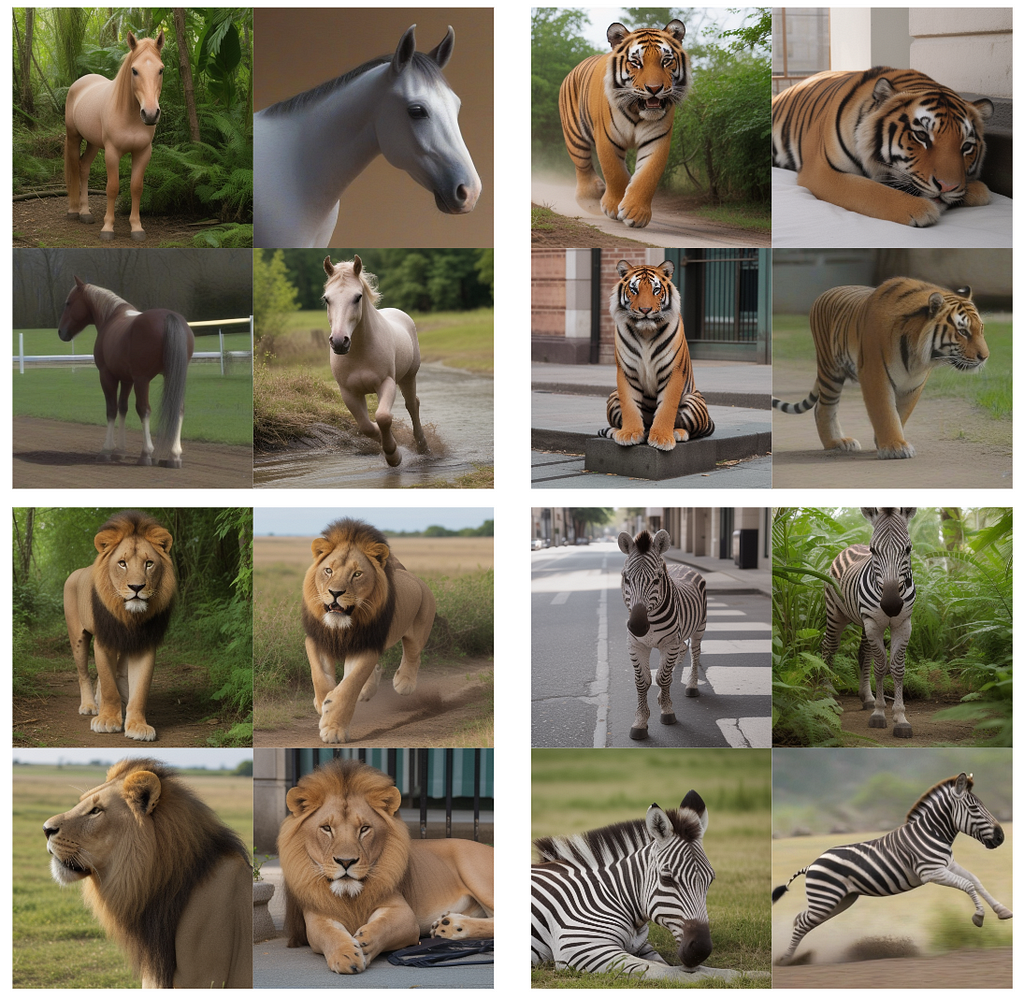
    All in all, it would generate images for 4 animals, 5 actions and 6 locations: so 120 possibilities. Adding to that, I used a batch count of 2 and 2 different models, increasing the generated images to 480 to create my dataset (120 for each animal class). Below are some examples of the generated images.

    Samples of the generated images using Stable Diffusion. Image by author.

    As we can see, most of the pictures are realistic enough. We will now get the instance masks, so that we can then train a segmentation model.

    Getting the labels

    To get the labels, we will use SAM model to generate masks, and we will then manually filter out masks that are not good enough, as well as unrealistic images (often called hallucinations).

    Generating the raw masks

    To generate the raw masks, let’s use SAM model. The SAM model requires input prompts (not a textual prompt): either a bounding box or a few point locations. This allows the model to generate the mask from this input prompt.

    In our case, we will do the most simple input prompt: the center point. Indeed, in most images generated by Stable Diffusion, the main object is centered, allowing us to efficiently use SAM with always the same input prompt and absolutely no labeling. To do so, we use the following function:

    This function will first instantiate a SAM predictor, given a model type and a checkpoint (to download here). It will then loop over the images in the input folder and do the following:

    • Load the image
    • Compute the mask thanks to SAM, with both the options multimask_output set to True and False
    • Apply closing to the mask before writing it as an image

    A few things to note:

    • We use both options multimask_output set to True and False because no option gives consistently superior results
    • We apply closing to the masks, because raw masks sometimes have a few holes

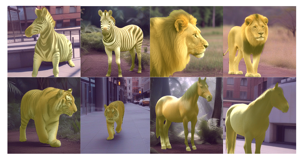
    Here are a few examples of images with their masks:

    A few images with the generated SAM masks displayed as a yellowish overlay. Image by author.

    As we can see, once selected, the masks are quite accurate and it took virtually no time to label.

    Selecting the masks

    Not all the masks were correctly computed in the previous subsection. Indeed, sometimes the object was not centered, thus the mask prediction was off. Sometimes, for some reason, the mask is just wrong and would need more input prompts to make it work.

    One quick workaround is to simply either select the best mask between the 2 computed ones, or simply remove the image from the dataset if no mask was good enough. Let’s do that with the following code:

    This code loops over all the generated images with Stable Diffusion and does the following for each image:

    • Load the two generated SAM masks
    • Display the image twice, one with each masks as an overlay, side by side
    • Waits for a keyboard event to make the selection

    The expected keyboard events are the following:

    • Left arrow of the keyboard to select the left mask
    • Right arrow to select the left mask
    • Down arrow to discard this image

    Running this script may take some time, since you have to go through all the images. Assuming 1 second per image, it would take about 10 minutes for 600 images. This is still much faster than actually labeling images with masks, that usually takes at least 30 second per mask for high quality masks. Moreover, this allows to effectively filter out any unrealistic image.

    Running this script on the generated 480 images took me less than 5 minutes. I selected the masks and filtered unrealistic images, so that I ended up with 412 masks. Next step is to train the model.

    Training the model

    Before training the YOLO segmentation model, we need to create the dataset properly. Let’s go through these steps.

    Creating the dataset

    This code loops through all the image and does the following:

    • Randomly select the train or validation set
    • Convert the masks to polygons for YOLO expected input label
    • Copy the image and the label in the right folders

    One tricky part in this code is in the mask to polygon conversion, done by the mask2yolo function. This makes use of shapely and rasterio libraries to make this conversion efficiently. Of course, you can find the fully working in the repository.

    In the end, you would end up with the following structure in your datasets folder:

    Folder structure after creating the dataset. Image by author.

    This is the expected structure to train a model using the YOLOv8 library: it’s finally time to train the model!

    Training the model

    We can now train the model. Let’s use a YOLOv8 nano segmentation model. Training a model is just two lines of code with the Ultralytics library, as we can see in the following gist:

    After 15 epochs of training on the previously prepared dataset, the results are the following:

    Results generated by YOLOv8 library after 15 epochs.

    As we can see, the metrics are quite high with a mAP50–95 close to 1, suggesting good performances. Of course, the dataset diversity being quite limited, those good performances are mostly likely caused by overfitting in some extent.

    For a more realistic evaluation, next we’ll evaluate the model on a few real images.

    Evaluating the model on real data

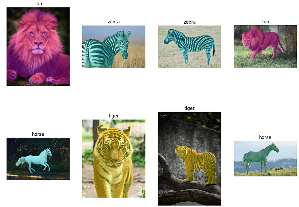
    From Unsplash, I got a few images from each class and tested the model on this data. The results are right below:

    Segmentation and class prediction results on real images from Unsplash.

    On these 8 real images, the model performed quite well: the animal class is successfully predicted, and the mask seems quite accurate. Of course, to evaluate properly this model, we would need a proper labeled dataset images and segmentation masks of each class.

    Conclusion

    With absolutely no images and no labels, we could train a segmentation model for 4 classes: horse, lion, tiger and zebra. To do so, we leveraged three amazing tools:

    • Stable diffusion to generate realistic images
    • SAM to compute the accurate masks of the objects
    • YOLOv8 to efficiently train an instance segmentation model

    While we couldn’t properly evaluate the trained model because we lack a labeled test dataset, it seems promising on a few images. Do not take this post as self-sufficient way to train any instance segmentation, but more as a method to speed up and boost the performances in your next projects. From my own experience, the use of synthetic data and tools like SAM can greatly improve your productivity in building production-grade computer vision models.

    Of course, all the code to do this on your own is fully available in this repository, and will hopefully help you in your next computer vision project!


    How to Train an Instance Segmentation Model with No Training Data was originally published in Towards Data Science on Medium, where people are continuing the conversation by highlighting and responding to this story.

    Originally appeared here:
    How to Train an Instance Segmentation Model with No Training Data

    Go Here to Read this Fast! How to Train an Instance Segmentation Model with No Training Data

  • Benchmark and optimize endpoint deployment in Amazon SageMaker JumpStart 

    Benchmark and optimize endpoint deployment in Amazon SageMaker JumpStart 

    Kyle Ulrich

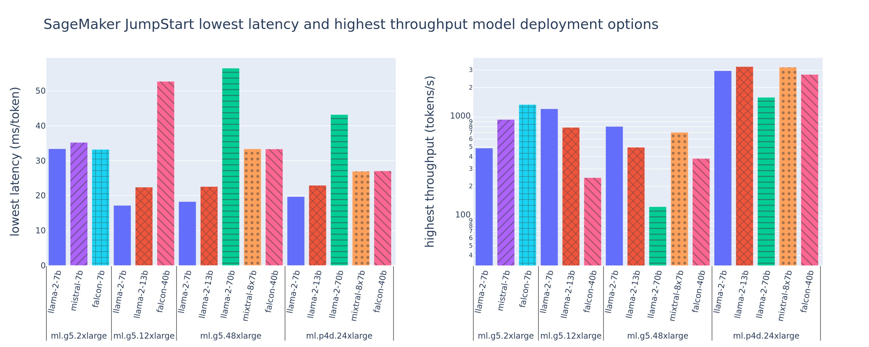
    When deploying a large language model (LLM), machine learning (ML) practitioners typically care about two measurements for model serving performance: latency, defined by the time it takes to generate a single token, and throughput, defined by the number of tokens generated per second. Although a single request to the deployed endpoint would exhibit a throughput […]

    Originally appeared here:
    Benchmark and optimize endpoint deployment in Amazon SageMaker JumpStart 

    Go Here to Read this Fast! Benchmark and optimize endpoint deployment in Amazon SageMaker JumpStart 

  • Mixed-input matrix multiplication performance optimizations

    Mixed-input matrix multiplication performance optimizations

    Google AI

    AI-driven technologies are weaving themselves into the fabric of our daily routines, with the potential to enhance our access to knowledge and boost our overall productivity. The backbone of these applications lies in large language models (LLMs). LLMs are memory-intensive and typically require specialized hardware accelerators to efficiently deliver tens of exaflops of computing power. This blog post shows how we can start addressing the computational challenges by utilizing memory more effectively.

    The bulk of an LLM’s memory and compute are consumed by weights in matrix multiplication operations. Using narrower data types reduces memory consumption. For example, storing weights in the 8-bit integer (i.e., U8 or S8) data type reduces the memory footprint by 4× relative to single-precision (F32) and 2× relative to half-precision (F16) or bfloat16 (BF16). Furthermore, previous work has shown that LLM models running matrix multiplications with weights in S8 and input in F16 (preserving higher precision of the user-input) is an effective method for increasing the efficiency with acceptable trade-offs in accuracy. This technique is known as weight-only quantization and requires efficient implementation of matrix multiplication with mixed-inputs, e.g., half-precision input multiplied with 8-bits integer. Hardware accelerators, including GPUs, support a fixed set of data types, and thus, mixed-input matrix multiplication requires software transformations to map to the hardware operations.

    To that end, in this blog we focus on mapping mixed-input matrix multiplication onto the NVIDIA Ampere architecture. We present software techniques addressing data type conversion and layout conformance to map mixed-input matrix multiplication efficiently onto hardware-supported data types and layouts. Our results show that the overhead of additional work in software is minimal and enables performance close to the peak hardware capabilities. The software techniques described here are released in the open-source NVIDIA/CUTLASS repository.

    Memory footprint for an 175B parameter LLM model with various data types formats.

    The matrix-multiply-accumulate operation

    Modern AI hardware accelerators such as Google’s TPU and NVIDIA’s GPU multiply matrices natively in the hardware by targeting Tensor Cores, which are specialized processing elements to accelerate matrix operations, particularly for AI workloads. In this blog, we focus on NVIDIA Ampere Tensor Cores, which provide the matrix-multiply-accumulate (mma) operation. For the rest of the blog the reference to mma is for Ampere Tensor Cores. The supported data types, shapes, and data layout of the two input matrices (called operands) for the mma operation are fixed in hardware. This means that matrix multiplications with various data types and larger shapes are implemented in the software by tiling the problem onto hardware-supported data types, shapes, and layouts.

    The Tensor Core mma operation is defined by specifying two input matrices (e.g., A & B, shown below) to produce a result matrix, C. The mma operation natively supports mixed-precision. Mixed-precision Tensor Cores allow mixing input (A and B) data type with the result (C) data type. In contrast, mixed-input matrix multiplication involves mixing the input data types, and it is not supported by the hardware, so it needs to be implemented in the software.

    Tensor Core operation of M-by-N-by-K on input matrix A of M-by-K and matrix B of K-by-N produces output matrix C of M-by-N.

    Challenges of mixed-input matrix multiplication

    To simplify the discussion, we restrict to a specific example of mixed-input matrix multiplication: F16 for user input and U8 for the model weights (written as F16 * U8). The techniques described here work for various combinations of mixed-input data types.

    A GPU programmer can access a hierarchy of memory, including global memory, shared memory, and registers, which are arranged in order of decreasing capacity but increasing speed. NVIDIA Ampere Tensor Core mma operations consume input matrices from registers. Furthermore, input and output matrices are required to conform to a layout of data within a group of 32 threads known as a warp. The supported data type and layout within a warp are fixed for an mma operation, so to implement mixed-input multiplication efficiently, it is necessary to solve the challenges of data type conversion and layout conformance in software.

    Data type conversion

    The mma operation requires two input matrices with the same data type. Thus, mixed-input matrix multiplication, where one of the operands is stored in U8 in global memory and other in F16, requires a data type conversion from U8 to F16. The conversion will bring two operands to F16, mapping the mixed-input matrix multiplication to hardware-supported mixed-precision Tensor Cores. Given the large number of weights, there are a large number of such operations, and our techniques show how to reduce their latency and improve performance.

    Layout conformance

    The mma operation also requires the layout of two input matrices, within the registers of a warp, to be conformat with hardware specification. The layout for the input matrix B of U8 data type in mixed-input matrix multiplication (F16 * U8) needs to conform with the converted F16 data type. This is called layout conformance and needs to be achieved in the software.

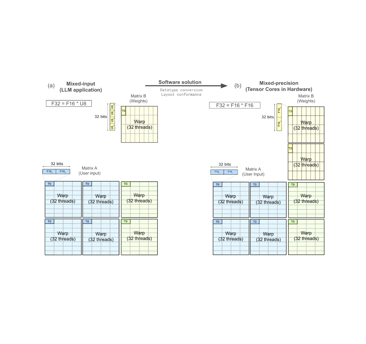
    The figure below shows an mma operation consuming matrix A and matrix B from registers to produce matrix C in registers, distributed across one warp. The thread T0 is highlighted and zoomed in to show the weight matrix B goes through data type conversion and needs a layout conformance to be able to map to the hardware-supported Tensor Core operation.

    The mapping of mixed-input (F32 = F16 * U8) operation in software to natively supported warp-level Tensor Cores in hardware (F32 = F16 * F16). (Original figure source Developing CUDA kernels to push Tensor Cores to the Absolute Limit on NVIDIA A100.)

    Software strategies addressing challenges

    A typical data type conversion involves a sequence of operations on 32-bit registers, shown below. Each rectangular block represents a register and the adjoining text are the operations. The entire sequence shows the conversion from 4xU8 to 2x(2xF16). The sequence involves roughly 10 operations.

    NumericArrayConvertor from 4xU8 to 2x(2xF16) in 32-bit registers.

    There are many ways of achieving layout conformance. Two of the existing solutions are:

    1. Narrower bitwidth shared memory loads: In this approach, threads issue narrow bitwidth memory loads moving the U8 data from shared memory to registers. This results in two 32-bit registers, with each register containing 2xF16 values (shown above for the matrix B’s thread T0). The narrower shared memory load achieves layout conformance directly into registers without needing any shuffles; however, it does not utilize the full shared memory bandwidth.
    2. Pre-processing in global memory: An alternative strategy involves rearranging the data within the global memory (one level above the shared memory in memory hierarchy), allowing wider shared memory loads. This approach maximizes the shared memory bandwidth utilization and ensures that the data is loaded in a conformant layout directly in the registers. Although the rearrangement process can be executed offline prior to the LLM deployment, ensuring no impact on the application performance, it introduces an additional, non-trivial hardware-specific pre-processing step that requires an extra program to rearrange the data. NVIDIA/FasterTransformer adopts this method to effectively address layout conformance challenges.

    Optimized software strategies

    To further optimize and reduce the overhead of data type conversion and layout conformance, we have implemented FastNumericArrayConvertor and FragmentShuffler, respectively.

    FastNumericArrayConvertor operates on 4xU8 in 32-bit registers without unpacking individual 1xU8 values. Furthermore, it uses less expensive arithmetic operations which reduces the number of instructions and increases the speed of the conversion.

    The conversion sequence for U8-to-F16 is shown below. The operations use packed 32b registers, avoiding explicit unpacking and packing. FastNumericArrayConvertor uses the permute byte to rearrange bytes of 4xU8 into two registers. Additionally, FastNumericArrayConvertor does not use expensive integer to floating-point conversion instructions and employs vectorized operations to obtain the packed results in two 32-bit registers containing 2x(2xF16) values. The FastNumericArrayConvertor for U8-to-F16 approximately uses six operations, a 1.6× reduction relative to the approach shown above.

    FastNumericArrayConvertor utilizes permute bytes and packed arithmetic, reducing the number of instructions in the data type conversion.

    FragmentShuffler handles the layout conformance by shuffling data in a way that allows the use of wider bitwidth load operation, increasing shared memory bandwidth utilization and reducing the total number of operations.

    NVIDIA Ampere architecture provides a load matrix instruction (ldmatrix). The ldmatrix is a warp-level operation, where 32 threads of a warp move the data from shared memory to registers in the shape and layout that mma matrix A and B consume. The use of ldmatrix reduces the number of load instructions and increases the memory bandwidth utilization. Since the ldmatrix instruction moves U8 data to registers, the layout after the load conforms with U8*U8 mma operation, and not with F16*F16 mma operation. We implemented FragmentShuffler to rearrange the data within registers using shuffle (shfl.sync) operations to achieve the layout conformance.

    The most significant contribution of this work is to achieve layout conformance through register shuffles, avoiding offline pre-processing in global memory or narrower bitwidth shared memory loads. Furthermore, we provide implementations for FastNumericArrayConvertor covering data type conversion from U8-to-F16, S8-to-F16, U8-to-BF16, and S8-to-BF16.

    Performance results

    We measured the performance of eight mixed-input variants of our method (shown below in blue and red; varying the data types of matrix A and B) and two mixed-precision data types (shown in green) on an NVIDIA A100 SXM chip. The performance results are shown in FLOPS (higher is better). Notably, the first eight matrix-multipications require additional operations relative to the last two, because the mixed-precision variants directly target hardware-accelerated Tensor Core operations and do not need data type conversion and layout conformance. Even so, our approach demonstrates mixed-input matrix multiplication performance only slightly below or on par with mixed-precision.

    Mixed-input matrix multiplication performance on NVIDIA A100 40GB SMX4 chip for a compute-bound matrix problem shape m=3456, n=4096, k=2048.

    Acknowledgements

    We would like to mention several folks who have contributed through technical brainstorming and improving the blog post including, Quentin Colombet, Jacques Pienaar, Allie Culp, Calin Cascaval, Ashish Gondimalla, Matt Walsh, Marek Kolodziej, and Aman Bhatia. We would like to thank our NVIDIA partners Rawn Henry, Pradeep Ramani, Vijay Thakkar, Haicheng Wu, Andrew Kerr, Matthew Nicely, and Vartika Singh.

    Originally appeared here:
    Mixed-input matrix multiplication performance optimizations

    Go Here to Read this Fast! Mixed-input matrix multiplication performance optimizations

  • Exphormer: Scaling transformers for graph-structured data

    Google AI

    Graphs, in which objects and their relations are represented as nodes (or vertices) and edges (or links) between pairs of nodes, are ubiquitous in computing and machine learning (ML). For example, social networks, road networks, and molecular structure and interactions are all domains in which underlying datasets have a natural graph structure. ML can be used to learn the properties of nodes, edges, or entire graphs.

    A common approach to learning on graphs are graph neural networks (GNNs), which operate on graph data by applying an optimizable transformation on node, edge, and global attributes. The most typical class of GNNs operates via a message-passing framework, whereby each layer aggregates the representation of a node with those of its immediate neighbors.

    Recently, graph transformer models have emerged as a popular alternative to message-passing GNNs. These models build on the success of Transformer architectures in natural language processing (NLP), adapting them to graph-structured data. The attention mechanism in graph transformers can be modeled by an interaction graph, in which edges represent pairs of nodes that attend to each other. Unlike message passing architectures, graph transformers have an interaction graph that is separate from the input graph. The typical interaction graph is a complete graph, which signifies a full attention mechanism that models direct interactions between all pairs of nodes. However, this creates quadratic computational and memory bottlenecks that limit the applicability of graph transformers to datasets on small graphs with at most a few thousand nodes. Making graph transformers scalable has been considered one of the most important research directions in the field (see the first open problem here).

    A natural remedy is to use a sparse interaction graph with fewer edges. Many sparse and efficient transformers have been proposed to eliminate the quadratic bottleneck for sequences, however, they do not generally extend to graphs in a principled manner.

    In “Exphormer: Sparse Transformers for Graphs”, presented at ICML 2023, we address the scalability challenge by introducing a sparse attention framework for transformers that is designed specifically for graph data. The Exphormer framework makes use of expander graphs, a powerful tool from spectral graph theory, and is able to achieve strong empirical results on a wide variety of datasets. Our implementation of Exphormer is now available on GitHub.

    Expander graphs

    A key idea at the heart of Exphormer is the use of expander graphs, which are sparse yet well-connected graphs that have some useful properties — 1) the matrix representation of the graphs have similar linear-algebraic properties as a complete graph, and 2) they exhibit rapid mixing of random walks, i.e., a small number of steps in a random walk from any starting node is enough to ensure convergence to a “stable” distribution on the nodes of the graph. Expanders have found applications to diverse areas, such as algorithms, pseudorandomness, complexity theory, and error-correcting codes.

    A common class of expander graphs are d-regular expanders, in which there are d edges from every node (i.e., every node has degree d). The quality of an expander graph is measured by its spectral gap, an algebraic property of its adjacency matrix (a matrix representation of the graph in which rows and columns are indexed by nodes and entries indicate whether pairs of nodes are connected by an edge). Those that maximize the spectral gap are known as Ramanujan graphs — they achieve a gap of d – 2*√(d-1), which is essentially the best possible among d-regular graphs. A number of deterministic and randomized constructions of Ramanujan graphs have been proposed over the years for various values of d. We use a randomized expander construction of Friedman, which produces near-Ramanujan graphs.

    Expander graphs are at the heart of Exphormer. A good expander is sparse yet exhibits rapid mixing of random walks, making its global connectivity suitable for an interaction graph in a graph transformer model.

    Exphormer replaces the dense, fully-connected interaction graph of a standard Transformer with edges of a sparse d-regular expander graph. Intuitively, the spectral approximation and mixing properties of an expander graph allow distant nodes to communicate with each other after one stacks multiple attention layers in a graph transformer architecture, even though the nodes may not attend to each other directly. Furthermore, by ensuring that d is constant (independent of the size of the number of nodes), we obtain a linear number of edges in the resulting interaction graph.

    Exphormer: Constructing a sparse interaction graph

    Exphormer combines expander edges with the input graph and virtual nodes. More specifically, the sparse attention mechanism of Exphormer builds an interaction graph consisting of three types of edges:

    • Edges from the input graph (local attention)
    • Edges from a constant-degree expander graph (expander attention)
    • Edges from every node to a small set of virtual nodes (global attention)
    Exphormer builds an interaction graph by combining three types of edges. The resulting graph has good connectivity properties and retains the inductive bias of the input dataset graph while still remaining sparse.

    Each component serves a specific purpose: the edges from the input graph retain the inductive bias from the input graph structure (which typically gets lost in a fully-connected attention module). Meanwhile, expander edges allow good global connectivity and random walk mixing properties (which spectrally approximate the complete graph with far fewer edges). Finally, virtual nodes serve as global “memory sinks” that can directly communicate with every node. While this results in additional edges from each virtual node equal to the number of nodes in the input graph, the resulting graph is still sparse. The degree of the expander graph and the number of virtual nodes are hyperparameters to tune for improving the quality metrics.

    Furthermore, since we use an expander graph of constant degree and a small constant number of virtual nodes for the global attention, the resulting sparse attention mechanism is linear in the size of the original input graph, i.e., it models a number of direct interactions on the order of the total number of nodes and edges.

    We additionally show that Exphormer is as expressive as the dense transformer and obeys universal approximation properties. In particular, when the sparse attention graph of Exphormer is augmented with self loops (edges connecting a node to itself), it can universally approximate continuous functions [1, 2].

    Relation to sparse Transformers for sequences

    It is interesting to compare Exphormer to sparse attention methods for sequences. Perhaps the architecture most conceptually similar to our approach is BigBird, which builds an interaction graph by combining different components. BigBird also uses virtual nodes, but, unlike Exphormer, it uses window attention and random attention from an Erdős-Rényi random graph model for the remaining components.

    Window attention in BigBird looks at the tokens surrounding a token in a sequence — the local neighborhood attention in Exphormer can be viewed as a generalization of window attention to graphs.

    The Erdős-Rényi graph on n nodes, G(n, p), which connects every pair of nodes independently with probability p, also functions as an expander graph for suitably high p. However, a superlinear number of edges (Ω(n log n)) is needed to ensure that an Erdős-Rényi graph is connected, let alone a good expander. On the other hand, the expanders used in Exphormer have only a linear number of edges.

    Experimental results

    Earlier works have shown the use of full graph Transformer-based models on datasets with graphs of size up to 5,000 nodes. To evaluate the performance of Exphormer, we build upon the celebrated GraphGPS framework [3], which combines both message passing and graph transformers and achieves state-of-the-art performance on a number of datasets. We show that replacing dense attention with Exphormer for the graph attention component in the GraphGPS framework allows one to achieve models with comparable or better performance, often with fewer trainable parameters.

    Furthermore, Exphormer notably allows graph transformer architectures to scale well beyond the usual graph size limits mentioned above. Exphormer can scale up to datasets of 10,000+ node graphs, such as the Coauthor dataset, and even beyond to larger graphs such as the well-known ogbn-arxiv dataset, a citation network, which consists of 170K nodes and 1.1 million edges.

    Results comparing Exphormer to standard GraphGPS on the five Long Range Graph Benchmark datasets. We note that Exphormer achieved state-of-the-art results on four of the five datasets (PascalVOC-SP, COCO-SP, Peptides-Struct, PCQM-Contact) at the time of the paper’s publication.

    Finally, we observe that Exphormer, which creates an overlay graph of small diameter via expanders, exhibits the ability to effectively learn long-range dependencies. The Long Range Graph Benchmark is a suite of five graph learning datasets designed to measure the ability of models to capture long-range interactions. Results show that Exphormer-based models outperform standard GraphGPS models (which were previously state-of-the-art on four out of five datasets at the time of publication).

    Conclusion

    Graph transformers have emerged as an important architecture for ML that adapts the highly successful sequence-based transformers used in NLP to graph-structured data. Scalability has, however, proven to be a major challenge in enabling the use of graph transformers on datasets with large graphs. In this post, we have presented Exphormer, a sparse attention framework that uses expander graphs to improve scalability of graph transformers. Exphormer is shown to have important theoretical properties and exhibit strong empirical performance, particularly on datasets where it is crucial to learn long range dependencies. For more information, we point the reader to a short presentation video from ICML 2023.

    Acknowledgements

    We thank our research collaborators Hamed Shirzad and Danica J. Sutherland from The University of British Columbia as well as Ali Kemal Sinop from Google Research. Special thanks to Tom Small for creating the animation used in this post.

    Originally appeared here:
    Exphormer: Scaling transformers for graph-structured data

    Go Here to Read this Fast! Exphormer: Scaling transformers for graph-structured data

  • Introducing ASPIRE for selective prediction in LLMs

    Introducing ASPIRE for selective prediction in LLMs

    Google AI

    In the fast-evolving landscape of artificial intelligence, large language models (LLMs) have revolutionized the way we interact with machines, pushing the boundaries of natural language understanding and generation to unprecedented heights. Yet, the leap into high-stakes decision-making applications remains a chasm too wide, primarily due to the inherent uncertainty of model predictions. Traditional LLMs generate responses recursively, yet they lack an intrinsic mechanism to assign a confidence score to these responses. Although one can derive a confidence score by summing up the probabilities of individual tokens in the sequence, traditional approaches typically fall short in reliably distinguishing between correct and incorrect answers. But what if LLMs could gauge their own confidence and only make predictions when they’re sure?

    Selective prediction aims to do this by enabling LLMs to output an answer along with a selection score, which indicates the probability that the answer is correct. With selective prediction, one can better understand the reliability of LLMs deployed in a variety of applications. Prior research, such as semantic uncertainty and self-evaluation, has attempted to enable selective prediction in LLMs. A typical approach is to use heuristic prompts like “Is the proposed answer True or False?” to trigger self-evaluation in LLMs. However, this approach may not work well on challenging question answering (QA) tasks.

    The OPT-2.7B model incorrectly answers a question from the TriviaQA dataset: “Which vitamin helps regulate blood clotting?” with “Vitamin C”. Without selective prediction, LLMs may output the wrong answer which, in this case, could lead users to take the wrong vitamin. With selective prediction, LLMs will output an answer along with a selection score. If the selection score is low (0.1), LLMs will further output “I don’t know!” to warn users not to trust it or verify it using other sources.

    In “Adaptation with Self-Evaluation to Improve Selective Prediction in LLMs“, presented at Findings of EMNLP 2023, we introduce ASPIRE — a novel framework meticulously designed to enhance the selective prediction capabilities of LLMs. ASPIRE fine-tunes LLMs on QA tasks via parameter-efficient fine-tuning, and trains them to evaluate whether their generated answers are correct. ASPIRE allows LLMs to output an answer along with a confidence score for that answer. Our experimental results demonstrate that ASPIRE significantly outperforms state-of-the-art selective prediction methods on a variety of QA datasets, such as the CoQA benchmark.

    The mechanics of ASPIRE

    Imagine teaching an LLM to not only answer questions but also evaluate those answers — akin to a student verifying their answers in the back of the textbook. That’s the essence of ASPIRE, which involves three stages: (1) task-specific tuning, (2) answer sampling, and (3) self-evaluation learning.

    Task-specific tuning: ASPIRE performs task-specific tuning to train adaptable parameters (θp) while freezing the LLM. Given a training dataset for a generative task, it fine-tunes the pre-trained LLM to improve its prediction performance. Towards this end, parameter-efficient tuning techniques (e.g., soft prompt tuning and LoRA) might be employed to adapt the pre-trained LLM on the task, given their effectiveness in obtaining strong generalization with small amounts of target task data. Specifically, the LLM parameters (θ) are frozen and adaptable parameters (θp) are added for fine-tuning. Only θp are updated to minimize the standard LLM training loss (e.g., cross-entropy). Such fine-tuning can improve selective prediction performance because it not only improves the prediction accuracy, but also enhances the likelihood of correct output sequences.

    Answer sampling: After task-specific tuning, ASPIRE uses the LLM with the learned θp to generate different answers for each training question and create a dataset for self-evaluation learning. We aim to generate output sequences that have a high likelihood. We use beam search as the decoding algorithm to generate high-likelihood output sequences and the Rouge-L metric to determine if the generated output sequence is correct.

    Self-evaluation learning: After sampling high-likelihood outputs for each query, ASPIRE adds adaptable parameters (θs) and only fine-tunes θs for learning self-evaluation. Since the output sequence generation only depends on θ and θp, freezing θ and the learned θp can avoid changing the prediction behaviors of the LLM when learning self-evaluation. We optimize θs such that the adapted LLM can distinguish between correct and incorrect answers on their own.

    The three stages of the ASPIRE framework.

    In the proposed framework, θp and θs can be trained using any parameter-efficient tuning approach. In this work, we use soft prompt tuning, a simple yet effective mechanism for learning “soft prompts” to condition frozen language models to perform specific downstream tasks more effectively than traditional discrete text prompts. The driving force behind this approach lies in the recognition that if we can develop prompts that effectively stimulate self-evaluation, it should be possible to discover these prompts through soft prompt tuning in conjunction with targeted training objectives.

    Implementation of the ASPIRE framework via soft prompt tuning. We first generate the answer to the question with the first soft prompt and then compute the learned self-evaluation score with the second soft prompt.

    After training θp and θs, we obtain the prediction for the query via beam search decoding. We then define a selection score that combines the likelihood of the generated answer with the learned self-evaluation score (i.e., the likelihood of the prediction being correct for the query) to make selective predictions.

    Results

    To demonstrate ASPIRE’s efficacy, we evaluate it across three question-answering datasets — CoQA, TriviaQA, and SQuAD — using various open pre-trained transformer (OPT) models. By training θp with soft prompt tuning, we observed a substantial hike in the LLMs’ accuracy. For example, the OPT-2.7B model adapted with ASPIRE demonstrated improved performance over the larger, pre-trained OPT-30B model using the CoQA and SQuAD datasets. These results suggest that with suitable adaptations, smaller LLMs might have the capability to match or potentially surpass the accuracy of larger models in some scenarios.

    When delving into the computation of selection scores with fixed model predictions, ASPIRE received a higher AUROC score (the probability that a randomly chosen correct output sequence has a higher selection score than a randomly chosen incorrect output sequence) than baseline methods across all datasets. For example, on the CoQA benchmark, ASPIRE improves the AUROC from 51.3% to 80.3% compared to the baselines.

    An intriguing pattern emerged from the TriviaQA dataset evaluations. While the pre-trained OPT-30B model demonstrated higher baseline accuracy, its performance in selective prediction did not improve significantly when traditional self-evaluation methods — Self-eval and P(True) — were applied. In contrast, the smaller OPT-2.7B model, when enhanced with ASPIRE, outperformed in this aspect. This discrepancy underscores a vital insight: larger LLMs utilizing conventional self-evaluation techniques may not be as effective in selective prediction as smaller, ASPIRE-enhanced models.

    Our experimental journey with ASPIRE underscores a pivotal shift in the landscape of LLMs: The capacity of a language model is not the be-all and end-all of its performance. Instead, the effectiveness of models can be drastically improved through strategic adaptations, allowing for more precise, confident predictions even in smaller models. As a result, ASPIRE stands as a testament to the potential of LLMs that can judiciously ascertain their own certainty and decisively outperform larger counterparts in selective prediction tasks.

    Conclusion

    In conclusion, ASPIRE is not just another framework; it’s a vision of a future where LLMs can be trusted partners in decision-making. By honing the selective prediction performance, we’re inching closer to realizing the full potential of AI in critical applications.

    Our research has opened new doors, and we invite the community to build upon this foundation. We’re excited to see how ASPIRE will inspire the next generation of LLMs and beyond. To learn more about our findings, we encourage you to read our paper and join us in this thrilling journey towards creating a more reliable and self-aware AI.

    Acknowledgments

    We gratefully acknowledge the contributions of Sayna Ebrahimi, Sercan O Arik, Tomas Pfister, and Somesh Jha.

    Originally appeared here:
    Introducing ASPIRE for selective prediction in LLMs

    Go Here to Read this Fast! Introducing ASPIRE for selective prediction in LLMs