Category: AI

Building a Chat Application with LangChain, LLMs, and Streamlit for Complex SQL Database Interaction

Build and deploy a chat application for complex database interaction with LangChain agents.

In this article we will see how we can use large language models (LLMs) to interact with a complex database using Langchain agents and tools, and then deploying the chat application using Streamlit.

This article is the second and final part of a two-phase project that exploits RappelConso API data, a French public service that shares information about product recalls in France.

In the first article, we set up a pipeline that queries the data from the API and stores it in a PostgreSQL database using various data engineering tools. In this article, we will develop a language model-based chat application that allows us to interact with the database.

Table of Contents

· Overview
· Set-up
· SQL Agent
· SQL Database Toolkit
· Extra tools
· Implementing Memory Features
· Creating the application with Streamlit
· Observations and enhancements
· Conclusion
· References

Overview

In this project, we’re going to create a chatbot that can talk to the RappelConso database through the Langchain framework. This chatbot will be able to understand natural language and use it to create and run SQL queries. We’ll enhance the chatbot’s ability to make SQL queries by giving it additional tools. It will also have a memory feature to remember past interactions with users. To make it user-friendly, we’ll use Streamlit to turn it into a chat-based web application.

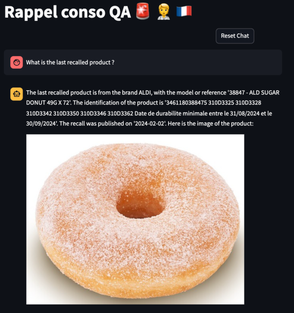
You can see a demo of the final application here:

The chatbot can answer queries with different complexities, from the categories count of the recalled products to specific questions about the products or brands. It can identify the right columns to query by using the tools at its disposal. The chatbot can also answer queries in “ASCII” compatible languages such as English, French, German, etc …

Glossary:

Here is a quick rundown of key terms to help you get a grasp of the concepts mentioned in this article.

• Langchain: LangChain is an open-source framework designed for building applications that leverage large language models (LLMs).
• Agents: They are components of Langchain that use a language model to determine which actions to take and in which order. The Agent has typically access to a set of functions called Tools and it can decide which Tool to use based on the user input.
• Tools: These are functions that an agent can invoke and enable it to interact with the world. Tools must be well described in a way that is most helpful to the agent.
• Toolkits: A set of related tools. In this project we will be using the SQLDatabaseToolkit. More on this in the subsequent sections.
• SQL Databases: The backbone holding the data you’ll be querying. In our project we will be using a Postgres Database.
• Streamlit: A python framework that enables the creation of interactive web applications very simply.

Now let’s dive into the technical details of this project !

Set-up

First you can clone the github repo with the following command:

git clone https://github.com/HamzaG737/rappel-conso-chat-app.git

Next, you can navigate to the project root and install the packages requirements:

pip install -r requirements.txt

In this project we experimented with two large language models from OpenAI, gpt-3.5-turbo-1106 and gpt-4–1106-preview . Since the latter is better at understanding and executing complex queries, we used it as the default LLM.

Setting-up the database

In my previous article, I covered how to set up a data pipeline for streaming data from a source API directly into a Postgres database. However, if you want a simpler solution, I created a script that allows you to transfer all the data from the API straight to Postgres, bypassing the need to set up the entire pipeline.

First off, you need to install Docker. Then you have to set the POSTGRES_PASSWORD as environment variable. By default, it will be set to the string “postgres” .

Next, get the Postgres server running with the docker-compose yaml file at the project’s root:

docker-compose -f docker-compose-postgres.yaml up -d

After that, the script database/stream_data.py helps you create the rappel_conso_table table, stream the data from the API into the database, and do a quick check on the data by counting the rows. As of February 2024, you should see around 10400 rows, so expect a number close to that.

To run the script, use this command:

python database/stream_data.py

Please note that the data transfer might take around one minute, possibly a little longer, depending on the speed of your internet connection.

The rappel_conso_table contains in total 25 columns, most of them are in TEXT type and can take infinite values. Some of the important columns are:

• reference_fiche (reference sheet): Unique identifier of the recalled product. It acts as the primary key of our Postgres database.
• categorie_de_produit (Product category): For instance food, electrical appliance, tools, transport means, etc …
• sous_categorie_de_produit (Product sub-category): For instance we can have meat, dairy products, cereals as sub-categories for the food category.
• motif_de_rappel (Reason for recall): Self explanatory and one of the most important fields.
• date_de_publication which translates to the publication date.
• risques_pour_le_consommateur which contains the risks that the consumer may encounter when using the product.
• There are also several fields that correspond to different links, such as link to product image, link to the distributers list, etc..

The full list of columns can be found in the constants.py file under the constant RAPPEL_CONSO_COLUMNS .

Given the wide range of columns present, it’s crucial for the agent to effectively distinguish between them, particularly in cases of ambiguous user queries. The SQLDatabaseToolkit, along with the additional tools we plan to implement, will play an important role in providing the necessary context. This context is key for the agent to accurately generate the appropriate SQL queries.

SQL Agent

LangChain has an SQL Agent which provides a flexible way of interacting with SQL Databases.

The benefits of employing the SQL Agent include:

• Its capability to respond to queries not only about the structure of the databases (such as details about a particular table) but also their content.
• Its ability to handle errors effectively. When an error occurs during the execution of a query, the SQL Agent can identify the issue, correct it, and then execute the revised query successfully.

In Langchain, we can initalize a SQL agent with the create_sql_agent function.

from langchain.agents import create_sql_agent

agent = create_sql_agent(
        llm=llm_agent,
        agent_type=AgentType.ZERO_SHOT_REACT_DESCRIPTION,
        toolkit=toolkit,
        verbose=True,
    )

• In this function, the llm is the large language model backbone of the agent. We chose OpenAI GPT models for this task but other models could also be suitable. Here is how we can define the LLM for the agent:

from langchain.chat_models import ChatOpenAI

from constants import chat_openai_model_kwargs, langchain_chat_kwargs

# Optional: set the API key for OpenAI if it's not set in the environment.
# os.environ["OPENAI_API_KEY"] = "xxxxxx"

def get_chat_openai(model_name):
    llm = ChatOpenAI(
        model_name=model_name,
        model_kwargs=chat_openai_model_kwargs,
        **langchain_chat_kwargs
    )
    return llm

• Currently, the create_sql_agent function supports two types of agents: OpenAI functions and ReAct agents. We opted for ReAct agents due to their easier integration with memory features. The ReAct agent model uses large language models to generate reasoning and task-specific actions together. This method helps the agent to plan, track, and adjust its actions while dealing with exceptions. It also enables the agent to connect with external sources like knowledge bases to get more information, improving its effectiveness in tasks. More details about this framework can be found here.

• Finally the toolkit in the create_sql_agent function represents the SQL set of tools used to interact with the database. More on this in the next section !

SQL Database Toolkit

The SQLDatabaseToolkit contains tools that can:

• Create and execute queries: In the following example, the ReAct agent will call the sql_db_query tool with a certain SQL query as input. Following this, it analyzes the database results to formulate an appropriate response for the user.

Action: sql_db_query
Action Input: SELECT reference_fiche, nom_de_la_marque_du_produit, noms_des_modeles_ou_references, date_de_publication, liens_vers_les_images FROM rappel_conso_table WHERE categorie_de_produit = 'Alimentation' ORDER BY date_de_publication DESC LIMIT 1
Observation: [('2024-01-0125', 'MAITRE COQ', 'Petite Dinde', '2024-01-13', 'https://rappel.conso.gouv.fr/image/ea3257df-7a68-4b49-916b-d6f019672ed2.jpg https://rappel.conso.gouv.fr/image/2a73be1e-b2ae-4a31-ad38-266028c6b219.jpg https://rappel.conso.gouv.fr/image/95bc9aa0-cc75-4246-bf6f-b8e8e35e2a88.jpg')]
Thought:I now know the final answer to the question about the last recalled food item.

Final Answer: The last recalled food item is "Petite Dinde" by the brand "MAITRE COQ", which was published on January 13, 2024. You can find the images of the recalled food item here: [lien vers l'image](https://rappel.conso.gouv.fr/image/ea3257df-7a68-4b49-916b-d6f019672ed2.jpg), [lien vers l'image](https://rappel.conso.gouv.fr/image/2a73be1e-b2ae-4a31-ad38-266028c6b219.jpg), [lien vers l'image](https://rappel.conso.gouv.fr/image/95bc9aa0-cc75-4246-bf6f-b8e8e35e2a88.jpg).

• Check the query syntax with the sql_db_query_checker tool.

Action: sql_db_query_checker
Action Input: SELECT reference_fiche, nom_de_la_marque_du_produit, noms_des_modeles_ou_references, date_de_publication, liens_vers_les_images FROM rappel_conso_table WHERE categorie_de_produit = 'Alimentation' ORDER BY date_de_publication DESC LIMIT 1
Observation: ```sql
SELECT reference_fiche, nom_de_la_marque_du_produit, noms_des_modeles_ou_references, date_de_publication, liens_vers_les_images FROM rappel_conso_table WHERE categorie_de_produit = 'Alimentation' ORDER BY date_de_publication DESC LIMIT 1
```
Thought:The query has been checked and is correct. I will now execute the query to find the last recalled food item.

• Retrieve table descriptions with the sql_db_schema tool.

Action: sql_db_schema
Action Input: rappel_conso_table
Observation: 
CREATE TABLE rappel_conso_table (
        reference_fiche TEXT NOT NULL, 
        liens_vers_les_images TEXT, 
        lien_vers_la_liste_des_produits TEXT, 
        lien_vers_la_liste_des_distributeurs TEXT, 
        lien_vers_affichette_pdf TEXT, 
        lien_vers_la_fiche_rappel TEXT, 
        date_de_publication TEXT, 
        date_de_fin_de_la_procedure_de_rappel TEXT, 
        categorie_de_produit TEXT, 
        sous_categorie_de_produit TEXT, 
        nom_de_la_marque_du_produit TEXT, 
        noms_des_modeles_ou_references TEXT, 
        identification_des_produits TEXT, 
        conditionnements TEXT, 
        temperature_de_conservation TEXT, 
        zone_geographique_de_vente TEXT, 
        distributeurs TEXT, 
        motif_du_rappel TEXT, 
        numero_de_contact TEXT, 
        modalites_de_compensation TEXT, 
        risques_pour_le_consommateur TEXT, 
        recommandations_sante TEXT, 
        date_debut_commercialisation TEXT, 
        date_fin_commercialisation TEXT, 
        informations_complementaires TEXT, 
        CONSTRAINT rappel_conso_table_pkey PRIMARY KEY (reference_fiche)
)

/*
1 rows from rappel_conso_table table:
reference_fiche liens_vers_les_images   lien_vers_la_liste_des_produits lien_vers_la_liste_des_distributeurs    lien_vers_affichette_pdf        lien_vers_la_fiche_rappel      date_de_publication     date_de_fin_de_la_procedure_de_rappel   categorie_de_produit    sous_categorie_de_produit       nom_de_la_marque_du_produit     noms_des_modeles_ou_references identification_des_produits     conditionnements        temperature_de_conservation     zone_geographique_de_vente      distributeurs   motif_du_rappel        numero_de_contact       modalites_de_compensation       risques_pour_le_consommateur    recommandations_sante   date_debut_commercialisation    date_fin_commercialisation     informations_complementaires
2021-04-0165    https://rappel.conso.gouv.fr/image/bd8027eb-ba27-499f-ba07-9a5610ad8856.jpg     None    None    https://rappel.conso.gouv.fr/affichettePDF/225/Internehttps://rappel.conso.gouv.fr/fiche-rappel/225/Interne    2021-04-22      mercredi 5 mai 2021     Alimentation    Cereales et produits de boulangerie     GERBLE BIO    BISCUITS 3 GRAINES BIO   3175681257535 11908141 Date de durabilite minimale 31/03/2022   ETUI CARTON 132 g       Produit a conserver a temperature ambiante      France entiere CASINO  Presence possible d'oxyde d'ethylene superieure a la limite autorisee sur un lot de matiere premiere    0805293032      Remboursement   Produits phytosanitaires non autorises Ne plus consommer Rapporter le produit au point de vente        19/03/2021      02/04/2021      None

Before defining the SQLDatabaseToolkit class, we must initialise the SQLDatabase wrapper around the Postgres database:

import os

from langchain.sql_database import SQLDatabase
from .constants_db import port, password, user, host, dbname


url = f"postgresql+psycopg2://{user}:{password}@{host}:{port}/{dbname}"
TABLE_NAME = "rappel_conso_table"

db = SQLDatabase.from_uri(
    url,
    include_tables=[TABLE_NAME],
    sample_rows_in_table_info=1,
)

The sample_rows_in_table_info setting determines how many example rows are added to each table’s description. Adding these sample rows can enhance the agent’s performance, as shown in this paper. Therefore, when the agent accesses a table’s description to gain a clearer understanding, it will obtain both the table’s schema and a sample row from that table.

Finally let’s define the SQL toolkit:

from langchain.agents.agent_toolkits import SQLDatabaseToolkit


def get_sql_toolkit(tool_llm_name):
    llm_tool = get_chat_openai(model_name=tool_llm_name)
    toolkit = SQLDatabaseToolkit(db=db, llm=llm_tool)
    return toolkit

Extra tools

Given the complexity of our table, the agent might not fully understand the information in the database by only examining the schema and a sample row. For example, the agent should recognise that a query regarding cars equates to searching the ‘category’ column for the value ‘Automobiles et moyens de déplacement’ (i.e., ‘Automobiles and means of transportation’). Therefore, additional tools are necessary to provide the agent with more context about the database.

Here’s a breakdown of the extra tools we plan to use:

• get_categories_and_sub_categories: This tool is designed to help the agent fetch a list of distinct items from the category and sub_category columns. This approach is effective due to the relatively low number of unique values within these columns. If the columns contained hundreds or thousands of unique values, it might be better to use a retrieval tool. In such cases, when a user asks about a category, the agent could look for the most similar categories in a vector database, which stores embeddings of various values. The agent would then use these categories for its SQL queries. However, given that our category and sub_category columns don’t have a wide range of unique values, we’ll simply return the list directly.

from langchain.tools import tool, Tool

import ast
import json

from sql_agent.sql_db import db


def run_query_save_results(db, query):
    res = db.run(query)
    res = [el for sub in ast.literal_eval(res) for el in sub]
    return res



def get_categories(query: str) -> str:
    """
    Useful to get categories and sub_categories. A json is returned where the key can be category or sub_category,
    and the value is a list of unique itmes for either both.
    """
    sub_cat = run_query_save_results(
        db, "SELECT DISTINCT sous_categorie_de_produit FROM rappel_conso_table"
    )
    cat = run_query_save_results(
        db, "SELECT DISTINCT categorie_de_produit FROM rappel_conso_table"
    )
    category_str = (
        "List of unique values of the categorie_de_produit column : n"
        + json.dumps(cat, ensure_ascii=False)
    )
    sub_category_str = (
        "n List of unique values of the sous_categorie_de_produit column : n"
        + json.dumps(sub_cat, ensure_ascii=False)
    )

    return category_str + sub_category_str

• get_columns_descriptions: Since we can’t feed the columns descriptions in the schema directly, we created an extra tool that returns short description for every ambiguous column. Some examples include:

"reference_fiche": "primary key of the database and unique identifier in the database. ",
"nom_de_la_marque_du_produit": "A string representing the Name of the product brand. Example: Apple, Carrefour, etc ... When you filter by this column,you must use LOWER() function to make the comparison case insensitive and you must use LIKE operator to make the comparison fuzzy.",
"noms_des_modeles_ou_references": "Names of the models or references. Can be used to get specific infos about the product. Example: iPhone 12, etc, candy X, product Y, bread, butter ...",
"identification_des_produits": "Identification of the products, for example the sales lot.",

def get_columns_descriptions(query: str) -> str:
    """
    Useful to get the description of the columns in the rappel_conso_table table.
    """
    return json.dumps(COLUMNS_DESCRIPTIONS)

• get_today_date : tool that retrieves today’s date using python datetime library. The agent will use this tool when asked about temporality. For example: “What are the recalled products since last week ?”

from datetime import datetime


def get_today_date(query: str) -> str:
    """
    Useful to get the date of today.
    """
    # Getting today's date in string format
    today_date_string = datetime.now().strftime("%Y-%m-%d")
    return today_date_string

Finally we create a list of all these tools and we feed it to the create_sql_agent function. For every tool we must define a unique name within the set of tools provided to the agent. The description is optional but is very recommended as it can be used to provide more information.

def sql_agent_tools():
    tools = [
        Tool.from_function(
            func=get_categories,
            name="get_categories_and_sub_categories",
            description="""
            Useful to get categories and sub_categories. A json is returned where the key can be category or sub_category, 
            and the value is a list of unique items for either both.
            """,
        ),
        Tool.from_function(
            func=get_columns_descriptions,
            name="get_columns_descriptions",
            description="""
            Useful to get the description of the columns in the rappel_conso_table table.
            """,
        ),
        Tool.from_function(
            func=get_today_date,
            name="get_today_date",
            description="""
            Useful to get the date of today.
            """,
        ),
    ]
    return tools

extra_tools = sql_agent_tools()

agent = create_sql_agent(
    llm=llm_agent,
    toolkit=toolkit,
    agent_type=AgentType.ZERO_SHOT_REACT_DESCRIPTION,
    extra_tools=extra_tools,
    verbose=True,
)

Sometimes, the tool descriptions aren’t enough for the agent to understand when to use them. To address this, we can change the ending part of the agent LLM prompt, known as the suffix. In our setup, the prompt has three sections:

1. Prefix: This is a string placed before the tool list. We’re sticking with the default prefix, which instructs the agent on how to create and execute SQL queries in response to user questions, set a limit on result numbers to 10 , check the queries carefully, and avoid making changes to the database.
2. The list of tools: This part lists out all the tools that the agent has at its disposal.
3. Suffix: This is the part where we give the agent directions on how to process and think about the user’s question.

Here’s the default suffix for the SQL ReAct agent in Langchain:

SQL_SUFFIX = """Begin!

Question: {input}
Thought: I should look at the tables in the database to see what I can query.  Then I should query the schema of the most relevant tables.
{agent_scratchpad}"""

input and agent_scratchpad are two placeholders. input represents the user’s query and agent_scratchpad will represent the history of tool invocations and the corresponding tool outputs.

We can make the “Thought” part longer to give more instructions on which tools to use and when:

CUSTOM_SUFFIX = """Begin!

Question: {input}
Thought Process: It is imperative that I do not fabricate information not present in the database or engage in hallucination; 
maintaining trustworthiness is crucial. If the user specifies a category, I should attempt to align it with the categories in the `categories_produits` 
or `sous_categorie_de_produit` columns of the `rappel_conso_table` table, utilizing the `get_categories` tool with an empty string as the argument. 
Next, I will acquire the schema of the `rappel_conso_table` table using the `sql_db_schema` tool. 
Utilizing the `get_columns_descriptions` tool is highly advisable for a deeper understanding of the `rappel_conso_table` columns, except for straightforward tasks. 
When provided with a product brand, I will search in the `nom_de_la_marque_du_produit` column; for a product type, in the `noms_des_modeles_ou_references` column. 
The `get_today_date` tool, requiring an empty string as an argument, will provide today's date. 
In SQL queries involving string or TEXT comparisons, I must use the `LOWER()` function for case-insensitive comparisons and the `LIKE` operator for fuzzy matching. 
Queries for currently recalled products should return rows where `date_de_fin_de_la_procedure_de_rappel` (the recall's ending date) is null or later than today's date. 
When presenting products, I will include image links from the `liens_vers_les_images` column, formatted strictly as:  [lien vers l'image] url1, [lien vers l'image] url2 ... Preceded by the mention in the query's language "here is(are) the image(s) :"
Additionally, the specific recalled product lot will be included from the `identification_des_produits` column. 
My final response must be delivered in the language of the user's query.

{agent_scratchpad}
"""

This way, the agent doesn’t just know what tools it has but also gets better guidance on when to use them.

Now let’s modify the arguments for the create_sql_agent to account for new suffix:

agent = create_sql_agent(
    llm=llm_agent,
    toolkit=toolkit,
    agent_type=AgentType.ZERO_SHOT_REACT_DESCRIPTION,
    suffix=CUSTOM_SUFFIX,
    extra_tools=agent_tools,
    verbose=True,
)

Another option we considered was to include the instructions in the prefix. However, our empirical observations indicated that this had little to no impact on the final response. Therefore, we chose to retain the instructions in the suffix. Conducting a more extensive evaluation of the model outputs could be beneficial for a detailed comparison of the two approaches.

Implementing Memory Features

A useful feature for our agent would be the ability to remember past interactions. This way, it doesn’t have to start over with each conversation, especially when queries are connected.

To add this memory feature, we’ll take a few steps:

• First, we import the ConversationBufferMemory class. This is a buffer that keeps track of the conversation history.

from langchain.memory import ConversationBufferMemory

memory = ConversationBufferMemory(memory_key="history", input_key="input")

• Next, we update the suffix to include the conversation history.

custom_suffix = """Begin!

Relevant pieces of previous conversation:
{history}
(Note: Only reference this information if it is relevant to the current query.)

Question: {input}
Thought Process: It is imperative that I do not fabricate information ... (same as previous suffix)

{agent_scratchpad}
"""

• Finally, we adjust the create_sql_agent function to add the history into the prompt placeholders and include the memory in the agent executor arguments.

agent = create_sql_agent(
    llm=llm_agent,
    toolkit=toolkit,
    agent_type=AgentType.ZERO_SHOT_REACT_DESCRIPTION,
    input_variables=["input", "agent_scratchpad", "history"],
    suffix=custom_suffix,
    agent_executor_kwargs={"memory": memory},
    extra_tools=agent_tools,
    verbose=True,
)

This way, the agent can use its memory to better handle related queries in a conversation.

Creating the application with Streamlit

We will use the python framework Streamlit to build a basic LLM chat app. Streamlit offers chat elements that can be used to construct a conversational application. The elements that we will use are:

• st.chat_input : a chat input widget that the user can use to type in a message.

• st.chat_message : This function adds a chat message to the app, displaying input from either the user or the application. The first argument specifies the message author, with “user” or “assistant” options to apply appropriate styling and avatars.

Additionally, we’ll utilize Streamlit’s session state to maintain a history of the conversation. This feature is crucial for providing a good user experience by preserving chat context.

More details on the process to create the conversational app can be found here.

Since we instructed the agent to always return the images urls, we created a post-processing function that fetches the images from these urls, formats the output, and displays the content using Streamlit’s markdown and image components. The implementation details for this functionality are available in the streamlit_app/gen_final_output.py module.

Now everything is set to start the chat application. You can execute the following command:

streamlit run streamlit_app/app.py

Future enhancements could include options for users to select the desired model and configure the OpenAI API key, further customizing the chat experience.

Observations and enhancements

Here are some insights we gained after running multiple dialogues with the agent:

• It’s not surprising, but GPT-4 is significantly better than GPT-3.5. The latter manages simple queries well but often struggles to invoke the necessary tools for additional context about the database, leading to frequent hallucinations.
• The complexity of the user’s question can make using GPT-4 both costly and slow. Generating detailed information like the database schema, row counts, and column descriptions uses a lot of tokens. Furthermore, if you’re looking for in-depth results, such as information on the last 10 recalled products, the agent has to process the query’s output along with the tools’ actions and observations, which can be very expensive. Therefore, it’s important to keep an eye on your usage to avoid unexpected costs.

To enhance the agent’s performance, we can:

• Refine how we engineer prompts, adjusting the suffix and/or prefix to better anticipate and efficiently invoke the right tools when needed.
• Include a few examples in the prompt, or employ a retrieval tool to find the most relevant examples for common user queries, reducing the need to repeatedly invoke the same tools for each new question.
• Add an evaluation framework to assess for instance the LLMs performance based on the final answer, or to compare prompts.

Conclusion

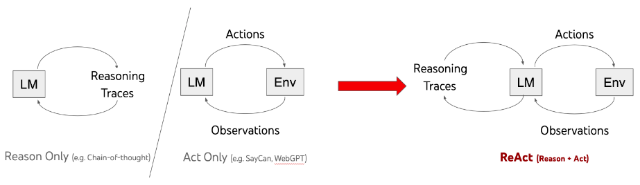
To wrap up, this article delved into creating a chat application that uses Large Language Models (LLMs) to communicate with SQL databases via the Langchain framework. We utilized the ReACT agent framework, along with various SQL tools and additional resources, to be able to respond to a wide range of user queries.

By incorporating memory capabilities and deploying via Streamlit, we’ve created a user-friendly interface that simplifies complex database queries into conversational exchanges.

Given the database’s complexity and the extensive number of columns it contains, our solution required a comprehensive set of tools and a powerful LLM.

We already talked about ways to enhance the capabilities of the chatbot. Additionally, using an LLM fine-tuned on SQL queries can be a substitute approach to using a general model like GPT. This could make the system much better at working with databases, helping it get even better at figuring out and handling tough queries.

References

• [2210.03629] ReAct: Synergizing Reasoning and Acting in Language Models (arxiv.org)
• Langchain SQL database
• Langchain SQL agent
• Langchain agents and tools documentation
• Build a basic LLM chat app with Streamlit
• An article on LLMs and SQL on Langchain’s blog.

---

Building a Chat App with LangChain, LLMs, and Streamlit for Complex SQL Database Interaction was originally published in Towards Data Science on Medium, where people are continuing the conversation by highlighting and responding to this story.

This article is part of a project that’s split into two main phases. The first phase focuses on building a data pipeline. This involves getting data from an API and storing it in a PostgreSQL database. In the second phase, we’ll develop an application that uses a language model to interact with this database.

Ideal for those new to data systems or language model applications, this project is structured into two segments:

• This initial article guides you through constructing a data pipeline utilizing Kafka for streaming, Airflow for orchestration, Spark for data transformation, and PostgreSQL for storage. To set-up and run these tools we will use Docker.
• The second article, which will come later, will delve into creating agents using tools like LangChain to communicate with external databases.

This first part project is ideal for beginners in data engineering, as well as for data scientists and machine learning engineers looking to deepen their knowledge of the entire data handling process. Using these data engineering tools firsthand is beneficial. It helps in refining the creation and expansion of machine learning models, ensuring they perform effectively in practical settings.

This article focuses more on practical application rather than theoretical aspects of the tools discussed. For detailed understanding of how these tools work internally, there are many excellent resources available online.

Overview

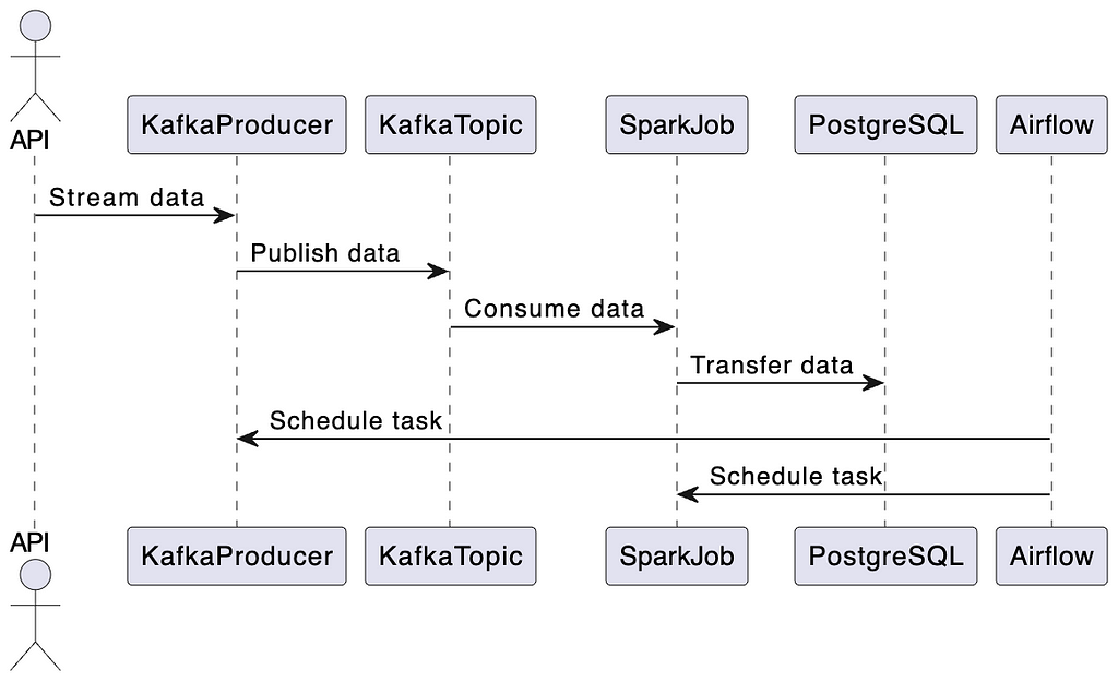
Let’s break down the data pipeline process step-by-step:

1. Data Streaming: Initially, data is streamed from the API into a Kafka topic.
2. Data Processing: A Spark job then takes over, consuming the data from the Kafka topic and transferring it to a PostgreSQL database.
3. Scheduling with Airflow: Both the streaming task and the Spark job are orchestrated using Airflow. While in a real-world scenario, the Kafka producer would constantly listen to the API, for demonstration purposes, we’ll schedule the Kafka streaming task to run daily. Once the streaming is complete, the Spark job processes the data, making it ready for use by the LLM application.

All of these tools will be built and run using docker, and more specifically docker-compose.

Now that we have a blueprint of our pipeline, let’s dive into the technical details !

Local setup

First you can clone the Github repo on your local machine using the following command:

git clone https://github.com/HamzaG737/data-engineering-project.git

Here is the overall structure of the project:

├── LICENSE
├── README.md
├── airflow
│   ├── Dockerfile
│   ├── __init__.py
│   └── dags
│       ├── __init__.py
│       └── dag_kafka_spark.py
├── data
│   └── last_processed.json
├── docker-compose-airflow.yaml
├── docker-compose.yml
├── kafka
├── requirements.txt
├── spark
│   └── Dockerfile
└── src
    ├── __init__.py
    ├── constants.py
    ├── kafka_client
    │   ├── __init__.py
    │   └── kafka_stream_data.py
    └── spark_pgsql
        └── spark_streaming.py

• The airflow directory contains a custom Dockerfile for setting up airflow and a dags directory to create and schedule the tasks.
• The data directory contains the last_processed.json file which is crucial for the Kafka streaming task. Further details on its role will be provided in the Kafka section.
• The docker-compose-airflow.yaml file defines all the services required to run airflow.
• The docker-compose.yaml file specifies the Kafka services and includes a docker-proxy. This proxy is essential for executing Spark jobs through a docker-operator in Airflow, a concept that will be elaborated on later.
• The spark directory contains a custom Dockerfile for spark setup.
• src contains the python modules needed to run the application.

To set up your local development environment, start by installing the required Python packages. The only essential package is psycopg2-binary. You have the option to install just this package or all the packages listed in the requirements.txt file. To install all packages, use the following command:

pip install -r requirements.txt

Next let’s dive step by step into the project details.

About the API

The API is RappelConso from the French public services. It gives access to data relating to recalls of products declared by professionals in France. The data is in French and it contains initially 31 columns (or fields). Some of the most important are:

• reference_fiche (reference sheet): Unique identifier of the recalled product. It will act as the primary key of our Postgres database later.
• categorie_de_produit (Product category): For instance food, electrical appliance, tools, transport means, etc …
• sous_categorie_de_produit (Product sub-category): For instance we can have meat, dairy products, cereals as sub-categories for the food category.
• motif_de_rappel (Reason for recall): Self explanatory and one of the most important fields.
• date_de_publication which translates to the publication date.
• risques_encourus_par_le_consommateur which contains the risks that the consumer may encounter when using the product.
• There are also several fields that correspond to different links, such as link to product image, link to the distributers list, etc..

You can see some examples and query manually the dataset records using this link.

We refined the data columns in a few key ways:

1. Columns like ndeg_de_version and rappelguid, which were part of a versioning system, have been removed as they aren’t needed for our project.
2. We combined columns that deal with consumer risks — risques_encourus_par_le_consommateur and description_complementaire_du_risque — for a clearer overview of product risks.
3. The date_debut_fin_de_commercialisation column, which indicates the marketing period, has been divided into two separate columns. This split allows for easier queries about the start or end of a product’s marketing.
4. We’ve removed accents from all columns except for links, reference numbers, and dates. This is important because some text processing tools struggle with accented characters.

For a detailed look at these changes, check out our transformation script at src/kafka_client/transformations.py. The updated list of columns is available insrc/constants.py under DB_FIELDS.

Kafka streaming

To avoid sending all the data from the API each time we run the streaming task, we define a local json file that contains the last publication date of the latest streaming. Then we will use this date as the starting date for our new streaming task.

To give an example, suppose that the latest recalled product has a publication date of 22 november 2023. If we make the hypothesis that all of the recalled products infos before this date are already persisted in our Postgres database, We can now stream the data starting from the 22 november. Note that there is an overlap because we may have a scenario where we didn’t handle all of the data of the 22nd of November.

The file is saved in ./data/last_processed.json and has this format:

{last_processed:"2023-11-22"}

By default the file is an empty json which means that our first streaming task will process all of the API records which are 10 000 approximately.

Note that in a production setting this approach of storing the last processed date in a local file is not viable and other approaches involving an external database or an object storage service may be more suitable.

The code for the kafka streaming can be found on ./src/kafka_client/kafka_stream_data.py and it involves primarily querying the data from the API, making the transformations, removing potential duplicates, updating the last publication date and serving the data using the kafka producer.

The next step is to run the kafka service defined the docker-compose defined below:

version: '3'

services:
  kafka:
    image: 'bitnami/kafka:latest'
    ports:
      - '9094:9094'
    networks:
      - airflow-kafka
    environment:
      - KAFKA_CFG_NODE_ID=0
      - KAFKA_CFG_PROCESS_ROLES=controller,broker
      - KAFKA_CFG_LISTENERS=PLAINTEXT://:9092,CONTROLLER://:9093,EXTERNAL://:9094
      - KAFKA_CFG_ADVERTISED_LISTENERS=PLAINTEXT://kafka:9092,EXTERNAL://localhost:9094
      - KAFKA_CFG_LISTENER_SECURITY_PROTOCOL_MAP=CONTROLLER:PLAINTEXT,EXTERNAL:PLAINTEXT,PLAINTEXT:PLAINTEXT
      - KAFKA_CFG_CONTROLLER_QUORUM_VOTERS=0@kafka:9093
      - KAFKA_CFG_CONTROLLER_LISTENER_NAMES=CONTROLLER
    volumes:
      - ./kafka:/bitnami/kafka

  kafka-ui:
    container_name: kafka-ui-1
    image: provectuslabs/kafka-ui:latest
    ports:
      - 8800:8080  
    depends_on:
      - kafka
    environment:
      KAFKA_CLUSTERS_0_NAME: local
      KAFKA_CLUSTERS_0_BOOTSTRAPSERVERS: PLAINTEXT://kafka:9092
      DYNAMIC_CONFIG_ENABLED: 'true'
    networks:
      - airflow-kafka


networks:
  airflow-kafka:
    external: true

The key highlights from this file are:

• The kafka service uses a base image bitnami/kafka.
• We configure the service with only one broker which is enough for our small project. A Kafka broker is responsible for receiving messages from producers (which are the sources of data), storing these messages, and delivering them to consumers (which are the sinks or end-users of the data). The broker listens to port 9092 for internal communication within the cluster and port 9094 for external communication, allowing clients outside the Docker network to connect to the Kafka broker.
• In the volumes part, we map the local directory kafka to the docker container directory /bitnami/kafka to ensure data persistence and a possible inspection of Kafka’s data from the host system.
• We set-up the service kafka-ui that uses the docker image provectuslabs/kafka-ui:latest . This provides a user interface to interact with the Kafka cluster. This is especially useful for monitoring and managing Kafka topics and messages.
• To ensure communication between kafka and airflow which will be run as an external service, we will use an external network airflow-kafka.

Before running the kafka service, let’s create the airflow-kafka network using the following command:

docker network create airflow-kafka

Now everything is set to finally start our kafka service

docker-compose up 

After the services start, visit the kafka-ui at http://localhost:8800/. Normally you should get something like this:

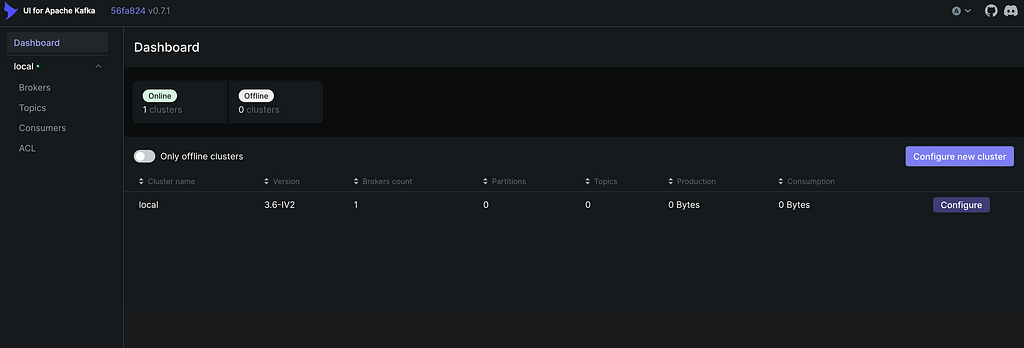
Next we will create our topic that will contain the API messages. Click on Topics on the left and then Add a topic at the top left. Our topic will be called rappel_conso and since we have only one broker we set the replication factor to 1. We will also set the partitions number to 1 since we will have only one consumer thread at a time so we won’t need any parallelism. Finally, we can set the time to retain data to a small number like one hour since we will run the spark job right after the kafka streaming task, so we won’t need to retain the data for a long time in the kafka topic.

Postgres set-up

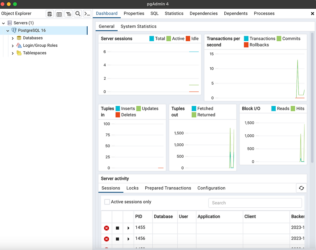
Before setting-up our spark and airflow configurations, let’s create the Postgres database that will persist our API data. I used the pgadmin 4 tool for this task, however any other Postgres development platform can do the job.

To install postgres and pgadmin, visit this link https://www.postgresql.org/download/ and get the packages following your operating system. Then when installing postgres, you need to setup a password that we will need later to connect to the database from the spark environment. You can also leave the port at 5432.

If your installation has succeeded, you can start pgadmin and you should observe something like this window:

Since we have a lot of columns for the table we want to create, we chose to create the table and add its columns with a script using psycopg2, a PostgreSQL database adapter for Python.

You can run the script with the command:

python scripts/create_table.py

Note that in the script I saved the postgres password as environment variable and name it POSTGRES_PASSWORD. So if you use another method to access the password you need to modify the script accordingly.

Spark Set-up

Having set-up our Postgres database, let’s delve into the details of the spark job. The goal is to stream the data from the Kafka topic rappel_conso to the Postgres table rappel_conso_table.

from pyspark.sql import SparkSession
from pyspark.sql.types import (
    StructType,
    StructField,
    StringType,
)
from pyspark.sql.functions import from_json, col
from src.constants import POSTGRES_URL, POSTGRES_PROPERTIES, DB_FIELDS
import logging


logging.basicConfig(
    level=logging.INFO, format="%(asctime)s:%(funcName)s:%(levelname)s:%(message)s"
)


def create_spark_session() -> SparkSession:
    spark = (
        SparkSession.builder.appName("PostgreSQL Connection with PySpark")
        .config(
            "spark.jars.packages",
            "org.postgresql:postgresql:42.5.4,org.apache.spark:spark-sql-kafka-0-10_2.12:3.5.0",

        )
        .getOrCreate()
    )

    logging.info("Spark session created successfully")
    return spark


def create_initial_dataframe(spark_session):
    """
    Reads the streaming data and creates the initial dataframe accordingly.
    """
    try:
        # Gets the streaming data from topic random_names
        df = (
            spark_session.readStream.format("kafka")
            .option("kafka.bootstrap.servers", "kafka:9092")
            .option("subscribe", "rappel_conso")
            .option("startingOffsets", "earliest")
            .load()
        )
        logging.info("Initial dataframe created successfully")
    except Exception as e:
        logging.warning(f"Initial dataframe couldn't be created due to exception: {e}")
        raise

    return df


def create_final_dataframe(df):
    """
    Modifies the initial dataframe, and creates the final dataframe.
    """
    schema = StructType(
        [StructField(field_name, StringType(), True) for field_name in DB_FIELDS]
    )
    df_out = (
        df.selectExpr("CAST(value AS STRING)")
        .select(from_json(col("value"), schema).alias("data"))
        .select("data.*")
    )
    return df_out


def start_streaming(df_parsed, spark):
    """
    Starts the streaming to table spark_streaming.rappel_conso in postgres
    """
    # Read existing data from PostgreSQL
    existing_data_df = spark.read.jdbc(
        POSTGRES_URL, "rappel_conso", properties=POSTGRES_PROPERTIES
    )

    unique_column = "reference_fiche"

    logging.info("Start streaming ...")
    query = df_parsed.writeStream.foreachBatch(
        lambda batch_df, _: (
            batch_df.join(
                existing_data_df, batch_df[unique_column] == existing_data_df[unique_column], "leftanti"
            )
            .write.jdbc(
                POSTGRES_URL, "rappel_conso", "append", properties=POSTGRES_PROPERTIES
            )
        )
    ).trigger(once=True) 
        .start()

    return query.awaitTermination()


def write_to_postgres():
    spark = create_spark_session()
    df = create_initial_dataframe(spark)
    df_final = create_final_dataframe(df)
    start_streaming(df_final, spark=spark)


if __name__ == "__main__":
    write_to_postgres()

Let’s break down the key highlights and functionalities of the spark job:

1. First we create the Spark session

def create_spark_session() -> SparkSession:
    spark = (
        SparkSession.builder.appName("PostgreSQL Connection with PySpark")
        .config(
            "spark.jars.packages",
            "org.postgresql:postgresql:42.5.4,org.apache.spark:spark-sql-kafka-0-10_2.12:3.5.0",

        )
        .getOrCreate()
    )

    logging.info("Spark session created successfully")
    return spark

2. The create_initial_dataframe function ingests streaming data from the Kafka topic using Spark’s structured streaming.

def create_initial_dataframe(spark_session):
    """
    Reads the streaming data and creates the initial dataframe accordingly.
    """
    try:
        # Gets the streaming data from topic random_names
        df = (
            spark_session.readStream.format("kafka")
            .option("kafka.bootstrap.servers", "kafka:9092")
            .option("subscribe", "rappel_conso")
            .option("startingOffsets", "earliest")
            .load()
        )
        logging.info("Initial dataframe created successfully")
    except Exception as e:
        logging.warning(f"Initial dataframe couldn't be created due to exception: {e}")
        raise

    return df

3. Once the data is ingested, create_final_dataframe transforms it. It applies a schema (defined by the columns DB_FIELDS) to the incoming JSON data, ensuring that the data is structured and ready for further processing.

def create_final_dataframe(df):
    """
    Modifies the initial dataframe, and creates the final dataframe.
    """
    schema = StructType(
        [StructField(field_name, StringType(), True) for field_name in DB_FIELDS]
    )
    df_out = (
        df.selectExpr("CAST(value AS STRING)")
        .select(from_json(col("value"), schema).alias("data"))
        .select("data.*")
    )
    return df_out

4. The start_streaming function reads existing data from the database, compares it with the incoming stream, and appends new records.

def start_streaming(df_parsed, spark):
    """
    Starts the streaming to table spark_streaming.rappel_conso in postgres
    """
    # Read existing data from PostgreSQL
    existing_data_df = spark.read.jdbc(
        POSTGRES_URL, "rappel_conso", properties=POSTGRES_PROPERTIES
    )

    unique_column = "reference_fiche"

    logging.info("Start streaming ...")
    query = df_parsed.writeStream.foreachBatch(
        lambda batch_df, _: (
            batch_df.join(
                existing_data_df, batch_df[unique_column] == existing_data_df[unique_column], "leftanti"
            )
            .write.jdbc(
                POSTGRES_URL, "rappel_conso", "append", properties=POSTGRES_PROPERTIES
            )
        )
    ).trigger(once=True) 
        .start()

    return query.awaitTermination()

The complete code for the Spark job is in the file src/spark_pgsql/spark_streaming.py. We will use the Airflow DockerOperator to run this job, as explained in the upcoming section.

Let’s go through the process of creating the Docker image we need to run our Spark job. Here’s the Dockerfile for reference:

FROM bitnami/spark:latest


WORKDIR /opt/bitnami/spark

RUN pip install py4j


COPY ./src/spark_pgsql/spark_streaming.py ./spark_streaming.py
COPY ./src/constants.py ./src/constants.py

ENV POSTGRES_DOCKER_USER=host.docker.internal
ARG POSTGRES_PASSWORD
ENV POSTGRES_PASSWORD=$POSTGRES_PASSWORD

In this Dockerfile, we start with the bitnami/spark image as our base. It’s a ready-to-use Spark image. We then install py4j, a tool needed for Spark to work with Python.

The environment variables POSTGRES_DOCKER_USER and POSTGRES_PASSWORD are set up for connecting to a PostgreSQL database. Since our database is on the host machine, we use host.docker.internal as the user. This allows our Docker container to access services on the host, in this case, the PostgreSQL database. The password for PostgreSQL is passed as a build argument, so it’s not hard-coded into the image.

It’s important to note that this approach, especially passing the database password at build time, might not be secure for production environments. It could potentially expose sensitive information. In such cases, more secure methods like Docker BuildKit should be considered.

Now, let’s build the Docker image for Spark:

docker build -f spark/Dockerfile -t rappel-conso/spark:latest --build-arg POSTGRES_PASSWORD=$POSTGRES_PASSWORD  .

This command will build the image rappel-conso/spark:latest . This image includes everything needed to run our Spark job and will be used by Airflow’s DockerOperator to execute the job. Remember to replace $POSTGRES_PASSWORD with your actual PostgreSQL password when running this command.

Airflow

As said earlier, Apache Airflow serves as the orchestration tool in the data pipeline. It is responsible for scheduling and managing the workflow of the tasks, ensuring they are executed in a specified order and under defined conditions. In our system, Airflow is used to automate the data flow from streaming with Kafka to processing with Spark.

Airflow DAG

Let’s take a look at the Directed Acyclic Graph (DAG) that will outline the sequence and dependencies of tasks, enabling Airflow to manage their execution.

start_date = datetime.today() - timedelta(days=1)


default_args = {
    "owner": "airflow",
    "start_date": start_date,
    "retries": 1,  # number of retries before failing the task
    "retry_delay": timedelta(seconds=5),
}


with DAG(
    dag_id="kafka_spark_dag",
    default_args=default_args,
    schedule_interval=timedelta(days=1),
    catchup=False,
) as dag:

    kafka_stream_task = PythonOperator(
        task_id="kafka_data_stream",
        python_callable=stream,
        dag=dag,
    )

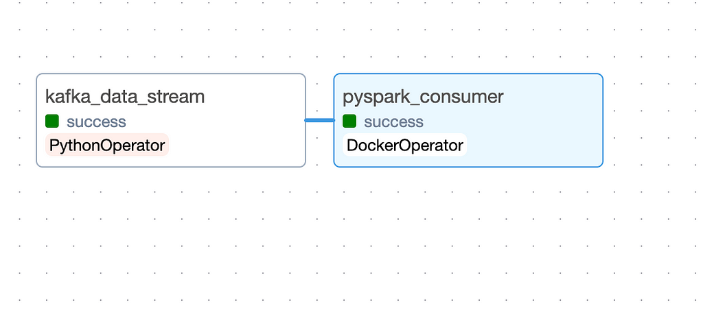
    spark_stream_task = DockerOperator(
        task_id="pyspark_consumer",
        image="rappel-conso/spark:latest",
        api_version="auto",
        auto_remove=True,
        command="./bin/spark-submit --master local[*] --packages org.postgresql:postgresql:42.5.4,org.apache.spark:spark-sql-kafka-0-10_2.12:3.5.0 ./spark_streaming.py",
        docker_url='tcp://docker-proxy:2375',
        environment={'SPARK_LOCAL_HOSTNAME': 'localhost'},
        network_mode="airflow-kafka",
        dag=dag,
    )


    kafka_stream_task >> spark_stream_task

Here are the key elements from this configuration

• The tasks are set to execute daily.
• The first task is the Kafka Stream Task. It is implemented using the PythonOperator to run the Kafka streaming function. This task streams data from the RappelConso API into a Kafka topic, initiating the data processing workflow.
• The downstream task is the Spark Stream Task. It uses the DockerOperator for execution. It runs a Docker container with our custom Spark image, tasked with processing the data received from Kafka.
• The tasks are arranged sequentially, where the Kafka streaming task precedes the Spark processing task. This order is crucial to ensure that data is first streamed and loaded into Kafka before being processed by Spark.

About the DockerOperator

Using docker operator allow us to run docker-containers that correspond to our tasks. The main advantage of this approach is easier package management, better isolation and enhanced testability. We will demonstrate the use of this operator with the spark streaming task.

Here are some key details about the docker operator for the spark streaming task:

• We will use the image rappel-conso/spark:latest specified in the Spark Set-up section.
• The command will run the Spark submit command inside the container, specifying the master as local, including necessary packages for PostgreSQL and Kafka integration, and pointing to the spark_streaming.py script that contains the logic for the Spark job.
• docker_url represents the url of the host running the docker daemon. The natural solution is to set it as unix://var/run/docker.sock and to mount the var/run/docker.sock in the airflow docker container. One problem we had with this approach is a permission error to use the socket file inside the airflow container. A common workaround, changing permissions with chmod 777 var/run/docker.sock, poses significant security risks. To circumvent this, we implemented a more secure solution using bobrik/socat as a docker-proxy. This proxy, defined in a Docker Compose service, listens on TCP port 2375 and forwards requests to the Docker socket:

  docker-proxy:
    image: bobrik/socat
    command: "TCP4-LISTEN:2375,fork,reuseaddr UNIX-CONNECT:/var/run/docker.sock"
    ports:
      - "2376:2375"
    volumes:
      - /var/run/docker.sock:/var/run/docker.sock
    networks:
      - airflow-kafka

In the DockerOperator, we can access the host docker /var/run/docker.sock via thetcp://docker-proxy:2375 url, as described here and here.

• Finally we set the network mode to airflow-kafka. This allows us to use the same network as the proxy and the docker running kafka. This is crucial since the spark job will consume the data from the kafka topic so we must ensure that both containers are able to communicate.

After defining the logic of our DAG, let’s understand now the airflow services configuration in the docker-compose-airflow.yaml file.

Airflow Configuration

The compose file for airflow was adapted from the official apache airflow docker-compose file. You can have a look at the original file by visiting this link.

As pointed out by this article, this proposed version of airflow is highly resource-intensive mainly because the core-executor is set to CeleryExecutor that is more adapted for distributed and large-scale data processing tasks. Since we have a small workload, using a single-noded LocalExecutor is enough.

Here is an overview of the changes we made on the docker-compose configuration of airflow:

• We set the environment variable AIRFLOW__CORE__EXECUTOR to LocalExecutor.
• We removed the services airflow-worker and flower because they only work for the Celery executor. We also removed the redis caching service since it works as a backend for celery. We also won’t use the airflow-triggerer so we remove it too.
• We replaced the base image ${AIRFLOW_IMAGE_NAME:-apache/airflow:2.7.3} for the remaining services, mainly the scheduler and the webserver, by a custom image that we will build when running the docker-compose.

version: '3.8'
x-airflow-common:
  &airflow-common
  build:
    context: .
    dockerfile: ./airflow_resources/Dockerfile
  image: de-project/airflow:latest

• We mounted the necessary volumes that are needed by airflow. AIRFLOW_PROJ_DIR designates the airflow project directory that we will define later. We also set the network as airflow-kafka to be able to communicate with the kafka boostrap servers.

volumes:
  - ${AIRFLOW_PROJ_DIR:-.}/dags:/opt/airflow/dags
  - ${AIRFLOW_PROJ_DIR:-.}/logs:/opt/airflow/logs
  - ${AIRFLOW_PROJ_DIR:-.}/config:/opt/airflow/config
  - ./src:/opt/airflow/dags/src
  - ./data/last_processed.json:/opt/airflow/data/last_processed.json
user: "${AIRFLOW_UID:-50000}:0"
networks:
  - airflow-kafka

Next, we need to create some environment variables that will be used by docker-compose:

echo -e "AIRFLOW_UID=$(id -u)nAIRFLOW_PROJ_DIR="./airflow_resources"" > .env

Where AIRFLOW_UID represents the User ID in Airflow containers and AIRFLOW_PROJ_DIR represents the airflow project directory.

Now everything is set-up to run your airflow service. You can start it with this command:

 docker compose -f docker-compose-airflow.yaml up

Then to access the airflow user interface you can visit this url http://localhost:8080 .

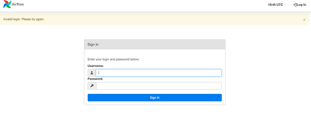
By default, the username and password are airflow for both. After signing in, you will see a list of Dags that come with airflow. Look for the dag of our project kafka_spark_dag and click on it.

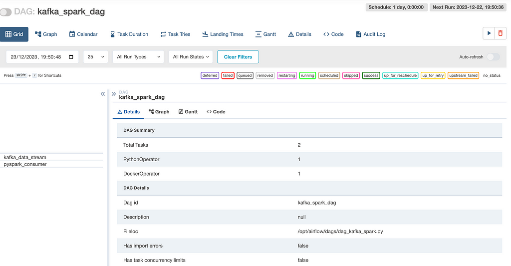
You can start the task by clicking on the button next to DAG: kafka_spark_dag.

Next, you can check the status of your tasks in the Graph tab. A task is done when it turns green. So, when everything is finished, it should look something like this:

To verify that the rappel_conso_table is filled with data, use the following SQL query in the pgAdmin Query Tool:

SELECT count(*) FROM rappel_conso_table

When I ran this in January 2024, the query returned a total of 10022 rows. Your results should be around this number as well.

Conclusion

This article has successfully demonstrated the steps to build a basic yet functional data engineering pipeline using Kafka, Airflow, Spark, PostgreSQL, and Docker. Aimed primarily at beginners and those new to the field of data engineering, it provides a hands-on approach to understanding and implementing key concepts in data streaming, processing, and storage.

Throughout this guide, we’ve covered each component of the pipeline in detail, from setting up Kafka for data streaming to using Airflow for task orchestration, and from processing data with Spark to storing it in PostgreSQL. The use of Docker throughout the project simplifies the setup and ensures consistency across different environments.

It’s important to note that while this setup is ideal for learning and small-scale projects, scaling it for production use would require additional considerations, especially in terms of security and performance optimization. Future enhancements could include integrating more advanced data processing techniques, exploring real-time analytics, or even expanding the pipeline to incorporate more complex data sources.

In essence, this project serves as a practical starting point for those looking to get their hands dirty with data engineering. It lays the groundwork for understanding the basics, providing a solid foundation for further exploration in the field.

In the second part, we’ll explore how to effectively use the data stored in our PostgreSQL database. We’ll introduce agents powered by Large Language Models (LLMs) and a variety of tools that enable us to interact with the database using natural language queries. So, stay tuned !

To reach out

• LinkedIn : https://www.linkedin.com/in/hamza-gharbi-043045151/
• Twitter : https://twitter.com/HamzaGh25079790

---

End-to-End Data Engineering System on Real Data with Kafka, Spark, Airflow, Postgres, and Docker was originally published in Towards Data Science on Medium, where people are continuing the conversation by highlighting and responding to this story.

How to Use LLMs and Controlled Vocabularies for Enhanced Similarity Models

The accompanying code for this tutorial is here.

Recommender systems are how we find much of the content and products we consume, probably including this article. A recommender system is:

“a subclass of information filtering system that provides suggestions for items that are most pertinent to a particular user.” — Wikipedia

Some examples of recommender systems we interact with regularly are on Netflix, Spotify, Amazon, and social media. All of these recommender systems are attempting to answer the same question: given a user’s past behavior, what other products or content are they most likely to like? These systems generate a lot of money — a 2013 study from McKinsey found that, “35 percent of what consumers purchase on Amazon and 75 percent of what they watch on Netflix come from product recommendations.” Netflix famously started an open competition in 2006 offering a one million dollar prize to anyone who could significantly improve their recommendation system. For more information on recommender systems see this article.

Generally, there are three kinds of recommender systems: content based, collaborative, and a hybrid of content based and collaborative. Collaborative recommender systems focus on users’ behavior and preferences to predict what they will like based on what other similar users like. Content based filtering systems focus on similarity between the products themselves rather than the users. For more info on these systems see this Nvidia piece.

Calculating similarity between products that are well-defined in a structured dataset is relatively straightforward. We could identify which properties of the products we think are most important, and measure the ‘distance’ between any two products given the difference between those properties. But what if we want to compare items when the only data we have is unstructured text? For example, given a dataset of movie and TV show descriptions, how can we calculate which are most similar?

In this tutorial, I will:

1. Show a basic similarity model (no controlled vocabulary) of unstructured text using natural language processing (NLP) techniques
2. Create a genre list using an LLM
3. Use the genre list to tag films with genres
4. Use the genre tags to build a similarity model
5. Use the genre tags to create a network visualization

The goal, for me, in writing this, was to learn two things: whether a taxonomy (controlled vocabulary) significantly improved the outcomes of a similarity model of unstructured data, and whether an LLM can significantly improve the quality and/or time required to construct that controlled vocabulary.

If you don’t feel like reading the whole thing, here are my main findings:

• The basic NLP model (without a controlled vocabulary) certainly has some problems — it sometimes uses words for identifying similar movies that are not relevant (like the protagonists’ first name or the location).
• Using a controlled vocabulary does significantly improve the outcomes of the similarity model, at least based on some of the examples I have been using to test the models.
• Building a simple, basic genre list using an LLM is easy — building a useful and/or detailed genre taxonomy is hard i.e. it would take more iterations or more descriptive prompts. I ended up building a quick and dirty list of about 200 genres without definitions, which worked good enough for doing simple similarity calculations.
• Even this very basic genre list built using an LLM has issues, however. There are duplicate genres with minor spelling differences, for example.
• Using an LLM to tag the movies and TV shows took a very long time. This might just be a problem in the way I have structured my code though.
• Perhaps not surprisingly, the depth and breadth of the taxonomy matters. Like I said above, building a detailed and descriptive taxonomy of movie genres is difficult and would require a lot more work than I am willing to do for this tutorial. But depending on the use case, that level of detail might not be necessary. I started by building a taxonomy of thousands of genres with synonyms and definitions but that had drawbacks — the tagging became harder and the similarity calculations were often not as good. Because I was only looking at a couple thousand movies, having a genre list of thousands of genres just made every movie unique and similar to almost nothing.
• Visualizing movies and genres as graphs is awesome, as always.

Basic Similarity Model of Unstructured Text Using NLP Techniques

We could use natural language processing (NLP) to extract key words from the text, identify how important these words are, and then find matching words in other descriptions. Here is a tutorial on how to do that in Python. I won’t recreate that entire tutorial here but here is a brief synopsis:

First, we extract key words from a plot description. For example, here is the description for the movie, ‘Indiana Jones and the Raiders of the Lost Ark.’

“When Indiana Jones is hired by the government to locate the legendary Ark of the Covenant, he finds himself up against the entire Nazi regime.”

We then use out-of-the-box libraries from sklearn to extract key words and rank their ‘importance’. To calculate importance, we use term-frequency-inverse document frequency (tf-idf). The idea is to balance the frequency of the term in the individual film’s description with how common the word is across all film descriptions in our dataset. The word ‘finds,’ for example, appears in this description, but it is a common word and appears in many other movie descriptions, so it is less important than ‘covenant’.

This model actually works very well for films that have a uniquely identifiable protagonist. If we run the similarity model on this film, the most similar movies are: ‘Indiana Jones and the Temple of Doom’, ‘Indiana Jones and the Last Crusade’, and ‘Indiana Jones and the Kingdom of the Crystal Skull’. This is because the descriptions for each of these movies contains the words, ‘Indiana’ and ‘Jones’.

But there are problems here. How do we know the words that are extracted and used in the similarity model are relevant? For example, if I run this model to find movies or TV shows similar to ‘Beavis and Butt-head Do America,” the top result is “Army of the Dead.” If you’re not a sophisticated film and TV buff like me, you may not be familiar with the animated series ‘Beavis and Butt-Head,’ featuring ‘unintelligent teenage boys [who] spend time watching television, drinking unhealthy beverages, eating, and embarking on mundane, sordid adventures, which often involve vandalism, abuse, violence, or animal cruelty.’ The description of their movie, ‘Beavis and Butt-head Do America,’ reads, ‘After realizing that their boob tube is gone, Beavis and Butt-head set off on an expedition that takes them from Las Vegas to the nation’s capital.’ ‘Army of the Dead,’ on the other hand, is a Zack Snyder-directed ‘post-apocalyptic zombie heist film’. Why is Army of the Dead considered similar then? Because it takes place in Las Vegas — both movie descriptions contain the words ‘Las Vegas’.

Another example of where this model fails is that if I want to find movies or TV shows similar to ‘Eat Pray Love,’ the top result is, ‘Extremely Wicked, Shockingly Evil and Vile.’ ‘Eat Pray Love’ is a romantic comedy starring Julia Roberts as Liz Gilbert, a recently divorced woman traveling the world in a journey of self-discovery. ‘Extremely Wicked, Shockingly Evil and Vile,’ is a true crime drama about serial killer Ted Bundy. What do these films have in common? Ted Bundy’s love interest is also named Liz.

These are, of course, cherry-picked examples of cases where this model doesn’t work. There are plenty of cases where extracting key words from text can be a useful way of finding similar products. As shown above, text that contains uniquely identifiable names like Power Rangers, Indiana Jones, or James Bond can be used to find other titles with those same names in their descriptions. Likewise, if the description contains information about the genre of the title, like ‘thriller’ or ‘mystery’, then those words can link the film to other films of the same genre. This has limitations too, however. Some films may use the word ‘dramatic’ in their description, but using this methodology, we would not match these films with film descriptions containing the word ‘drama’ — we are not accounting for synonyms. What we really want is to only use relevant words and their synonyms.

How can we ensure that the words extracted are relevant? This is where a taxonomy can help. What is a taxonomy?

Create a genre taxonomy using an LLM

“A taxonomy (or taxonomic classification) is a scheme of classification, especially a hierarchical classification, in which things are organized into groups or types.” — Wikipedia

Perhaps the most famous example of a taxonomy is the one used in biology to categorize all living organisms — remember domain, kingdom, phylum class, order, family, genus, and species? All living creatures can be categorized into this hierarchical taxonomy.

A note on terminology: ontologies are similar to taxonomies but different. As this article explains, taxonomies classify while ontologies specify. “An ontology is the system of classes and relationships that describe the structure of data, the rules, if you will, that prescribe how a new category or entity is created, how attributes are defined, and how constraints are established.” Since we are focused on classifying movies, we are going to build a taxonomy. However, for the purposes of this tutorial, I just need a very basic list of genres, which can’t even really be described as a taxonomy. A list of genres is just a tag set, or a controlled vocabulary.

For this tutorial, we will focus only on genre. What we need is a list of genres that we can use to ‘tag’ each movie. Imagine that instead of having the movie, ‘Eat Pray Love’ tagged with the words ‘Liz’ and ‘true’, it were tagged with ‘romantic comedy’, ‘drama’, and ‘travel/adventure’. We could then use these genres to find other movies similar to Eat Pray Love, even if the protagonist is not named Liz. Below is a diagram of what we are doing. We use a subset of the unstructured movie data, along with GPT 3.5, to create a list of genres. Then we use the genre list and GPT 3.5 to tag the unstructured movie data. Once our data is tagged, we can run a similarity model using the tags as inputs.

I couldn’t find any free movie genre taxonomies online, so I built my own using a large language model (LLM). I started with this tutorial, which used an LLM agent to build a taxonomy of job titles. That LLM agent looks for job titles from job descriptions, creates definitions and responsibilities for each of these job titles, and synonyms. I used that tutorial to create a movie genre taxonomy, but it was overkill — we don’t really need to do all of that for the purposes of this tutorial. We just need a very basic list of genres that we can use to tag movies. Here is the code I used to create that genre list.

I used Netflix movie and TV show description data available here (License CC0: Public Domain).

Import required packages and load english language NLP model.

import openai
import os
import re
import pandas as pd
import spacy
from ipywidgets import FloatProgress
from tqdm import tqdm

# Load English tokenizer, tagger, parser and NER
nlp = spacy.load("en_core_web_sm")

Then we need to set up our connection with OpenAI (or whatever LLM you want to use).

os.environ["OPENAI_API_KEY"] = "XXXXXX"  # replace with yours

Read in the Netflix movie data:

movies = pd.read_csv("netflix_titles.csv")
movies = movies.sample(n=1000) #I just used 1000 rows of data to reduce the runtime

Create a function to predict the genre of a title given its description:

def predict_genres(movie_description):
    prompt = f"Predict the top three genres (only genres, not descriptions) for a movie with the following description: {movie_description}"
    response = openai.completions.create(
      model="gpt-3.5-turbo-instruct",  # You can use the GPT-3 model for this task
      prompt=prompt,
      max_tokens=50,
      n=1,
      stop=None,
      temperature=0.2
    )
    predicted_genres = response.choices[0].text.strip()
    return predicted_genres

Now we iterate through our DataFrame of movie descriptions, use the function above to predict the genres associated with the movie, then add them to our list of established unique genres.

# Create an empty list to store the predicted genres
all_predicted_genres = []

# Create an empty set to store unique genres
unique_genres_set = set()

# Iterate through the movie descriptions
for index, row in tqdm(movies.iterrows(), total=movies.shape[0]):
    
        # Get the movie description
        movie_description = row['description']
    
        # Predict the genres for the movie description
        predicted_genres = predict_genres(movie_description)
    
        # Extract genres from the text
        predicted_genres_tokens = nlp(predicted_genres)
        predicted_genres_tokens = predicted_genres_tokens.text
        
        # Use regular expression to extract genres
        genres_with_numbers = re.findall(r'd+.s*([^n]+)', predicted_genres_tokens)
        
        # Remove leading/trailing whitespaces from each genre
        predicted_genres = [genre.strip().lower() for genre in genres_with_numbers]
    
        # Update the set of unique genres
        unique_genres_set.update(predicted_genres)

# Convert the set of unique genres back to a list
all_unique_genres = list(unique_genres_set)

Now turn this list into a DataFrame and save to a csv file:

all_unique_genres = pd.DataFrame(all_unique_genres,columns=['genre'])
all_unique_genres.to_csv("genres_taxonomy_quick.csv")

Like I said, this is a quick and dirty way to generate this list of genres.

Use the genre list to tag films with genres

Now that we have a list of genres, we need to tag each of the movies and TV shows in our dataset (over 8,000) with them. To be able to use these tags to calculate similarity between two entities, we need to tag each movie and TV show with more than one genre. If we only used one genre, then all action movies will be equally similar, even though some may be more about sports and others, horror.

First, we read in our genre list and movie dataset:

#Read in our genre list
genres = pd.read_csv('genres_taxonomy_quick.csv')  # Replace 'genres_taxonomy_quick.csv' with the actual file name
genres = genres['genre']

#Read in our movie data
movies = pd.read_csv("netflix_titles.csv")
movies = movies.sample(n=1000) #This takes a while to run so I didn't do it for the entire dataset at once

We already have a function for predicting genres. Now we need to define two more functions: one for filtering the predictions to ensure that the predictions are in our established genre list, and one for adding those filtered predictions to the movie DataFrame.

#Function to filter predicted genres
def filter_predicted_genres(predicted_genres, predefined_genres):
    # Use word embeddings to calculate semantic similarity between predicted and predefined genres
    predicted_genres_tokens = nlp(predicted_genres)
    predicted_genres_tokens = predicted_genres_tokens.text
    # Use regular expression to extract genres
    genres_with_numbers = re.findall(r'd+.s*([^n]+)', predicted_genres_tokens)
    # Remove leading/trailing whitespaces from each genre
    predicted_genres = [genre.strip().lower() for genre in genres_with_numbers]

    filtered_genres = []
    similarity_scores = []

    for predicted_genre in predicted_genres:
        max_similarity = 0
        best_match = None
        for predefined_genre in predefined_genres:
            similarity_score = nlp(predicted_genre).similarity(nlp(predefined_genre))
            if similarity_score > max_similarity:  # Adjust the threshold as needed
                max_similarity = similarity_score
                best_match = predefined_genre
        filtered_genres.append(best_match)
        similarity_scores.append(max_similarity)

    # Sort the filtered genres based on the similarity scores
    filtered_genres = [x for _, x in sorted(zip(similarity_scores, filtered_genres), reverse=True)]
    
    return filtered_genres

#Function to add filtered predictions to DataFrame
def add_predicted_genres_to_df(df, predefined_genres):   
    # Iterate through the dataframe
    for index, row in tqdm(df.iterrows(), total=df.shape[0]):
        # Apply the predict_genres function to the movie description
        predicted_genres = predict_genres(row['description'])
        # Prioritize the predicted genres
        filtered_genres = filter_predicted_genres(predicted_genres, predefined_genres)
        # Add the prioritized genres to the dataframe
        df.at[index, 'predicted_genres'] = filtered_genres

Once we have these functions defined, we can run them on our movies dataset:

add_predicted_genres_to_df(movies, genres)

Now we do some data cleaning:

# Split the lists into separate columns with specific names
movies[['genre1', 'genre2', 'genre3']] = movies['predicted_genres'].apply(lambda x: pd.Series((x + [None, None, None])[:3]))

#Keep only the columns we need for similarity
movies = movies[['title','genre1','genre2','genre3']]

#Drop duplicates
movies = movies.drop_duplicates()

#Set the 'title' column as our index
movies = movies.set_index('title')

If we print the head of the DataFrame it should look like this:

Use the genre tags to build a similarity model

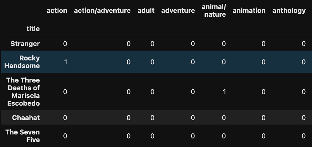
Now we turn the genre columns into dummy variables — each genre becomes its own column and if the movie or TV show is tagged with that genre then the column gets a 1, otherwise the value is 0.

# Combine genre columns into a single column
movies['all_genres'] = movies[['genre1', 'genre2', 'genre3']].astype(str).agg(','.join, axis=1)

# Split the genres and create dummy variables for each genre
genres = movies['all_genres'].str.get_dummies(sep=',')

# Concatenate the dummy variables with the original DataFrame
movies = pd.concat([movies, genres], axis=1)

# Drop unnecessary columns
movies.drop(['all_genres', 'genre1', 'genre2', 'genre3'], axis=1, inplace=True)

If we print the head of this DataFrame, this is what it looks like:

We need to use these dummy variables to build a matrix and run a similarity model across all pairs of movies:

# If there are duplicate columns due to the one-hot encoding, you can sum them up
movie_genre_matrix = movies.groupby(level=0, axis=1).sum()

# Calculate cosine similarity 
similarity_matrix = cosine_similarity(movie_genre_matrix, movie_genre_matrix)

Now we can define a function that calculates the most similar movies to a given title:

def find_similar_movies(movie_name, movie_genre_matrix, num_similar_movies=3):
    # Calculate cosine similarity
    similarity_matrix = cosine_similarity(movie_genre_matrix, movie_genre_matrix)
    
    # Find the index of the given movie
    movie_index = movie_genre_matrix.index.get_loc(movie_name)
    
    # Sort and get indices of most similar movies (excluding the movie itself)
    most_similar_indices = np.argsort(similarity_matrix[movie_index])[:-num_similar_movies-1:-1]
    
    # Return the most similar movies
    return movie_genre_matrix.index[most_similar_indices].tolist()

Let’s see if this model finds movies more similar to ‘Eat Pray Love,’ than the previous model:

# Example usage
similar_movies = find_similar_movies("Eat Pray Love", movie_genre_matrix, num_similar_movies=4)
print(similar_movies)

The output from this query, for me, were, ‘The Big Day’, ‘Love Dot Com: The Social Experiment’, and ’50 First Dates’. All of these movies are tagged as romantic comedies and dramas, just like Eat Pray Love.

‘Extremely Wicked, Shockingly Evil and Vile,’ the movie about a woman in love with Ted Bundy, is tagged with the genres romance, drama, and crime. The most similar movies are, ‘The Fury of a Patient Man’, ‘Much Loved’, and ‘Loving You’, all of which are also tagged with romance, drama, and crime. ‘Beavis and Butt-head Do America’ is tagged with the genres comedy, adventure and road trip. The most similar movies are ‘Pee-wee’s Big Holiday’, ‘A Shaun the Sheep Movie: Farmageddon’, and ‘The Secret Life of Pets 2.’ All of these movies are also tagged with the genres adventure and comedy — there are no other movies in this dataset (at least the portion I tagged) that match all three genres from Beavis and Butt-head.

Use the genre tags to create a network visualization

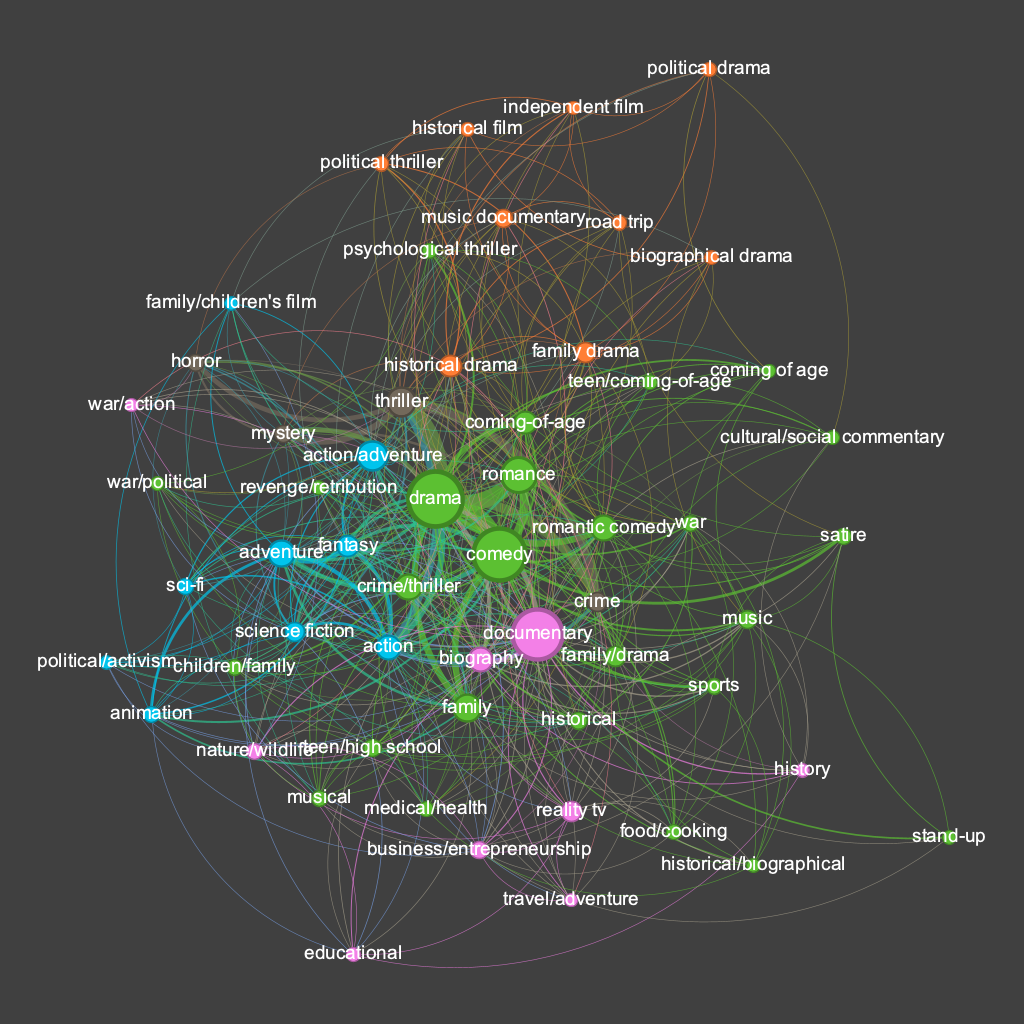
You can’t link data together without building a cool network visualization. There are a few ways to turn this data into a graph — we could look at how movies are conneted via genres, how genres are connected via movies, or a combination of the two. Because there are so many movies in this dataset, I just made a graph using genres as nodes and movies as edges.

Here is my code to turn the data into nodes and edges:

# Melt the dataframe to unpivot genre columns
melted_df = pd.melt(movies, id_vars=['title'], value_vars=['genre1', 'genre2', 'genre3'], var_name='Genre', value_name='GenreValue')

genre_links = pd.crosstab(index=melted_df['title'], columns=melted_df['GenreValue'])

# Create combinations of genres for each title
combinations_list = []

for title, group in melted_df.groupby('title')['GenreValue']:
    genre_combinations = list(combinations(group, 2))
    combinations_list.extend([(title, combo[0], combo[1]) for combo in genre_combinations])

# Create a new dataframe from the combinations list
combinations_df = pd.DataFrame(combinations_list, columns=['title', 'Genre1', 'Genre2'])

combinations_df = combinations_df[['Genre1','Genre2']]

combinations_df = combinations_df.rename(columns={"Genre1": "source", "Genre2": "target"}, errors="raise")

combinations_df = combinations_df.set_index('source')

combinations_df.to_csv("genreCombos.csv")

This produces a DataFrame that looks like this:

Each row in this DataFrame represents a movie that has been tagged with these two genres. We did not remove duplicates so there will be, presumably, many rows that look like row 1 above — there are many movies that are tagged as both romance and drama.

I used Gephi to build a visualization that looks like this:

The size of the nodes here represents the number of movies tagged with that genre. The color of the nodes is a function of a community detection algorithm — clusters that have closer connections amongst themselves than with nodes outside their cluster are colored the same.

This is fascinating to me. Drama, comedy, and documentary are the three largest nodes meaning more movies are tagged with those genres than any others. The genres also naturally form clusters that make intuitive sense. The genres most aligned with ‘documentary’ are colored pink and are mostly some kind of documentary sub-genre: nature/wildlife, reality TV, travel/adventure, history, educational, biography, etc. There are a core cluster of genres in green: drama, comedy, romance, coming of age, family, etc. One issue here is that we have multiple spellings of the ‘coming of age’ genre — a problem I would fix in future versions. There is a cluster in blue that includes action/adventure, fantasy, sci-fi, and animation. Again, we have duplicates and overlapping genres here which is a problem. There is also a small genre in brown that includes thriller, mystery, and horror — adult genres often present in the same film. The lack of connections between certain genres is also interesting — there are no films tagged with both ‘stand-up’ and ‘horror’, for example.

Conclusion

This project has shown me how even the most basic controlled vocabulary is useful, and potentially necessary, when building a content-based recommendation system. With just a list of genres we were able to tag movies and find other similar movies in a more explainable way than using just NLP. This could obviously be improved immensely through a more detailed and description genre taxonomy, but also through additional taxonomies including the cast and crew of films, the locations, etc.

As is usually the case when using LLMs, I was very impressed at first at how well it could perform this task, only to be disappointed when I viewed and tried to improve the results. Building taxonomies, ontologies, or any controlled vocabulary requires human engagement — there needs to be a human in the loop to ensure the vocabulary makes sense and will be useful in satisfying a particular use case.

LLMs and knowledge graphs (KGs) naturally fit together. One way they can be used together is that LLMs can help facilitate KG creation. LLMs can’t build a KG themselves but they can certainly help you create one.

---

Unraveling Unstructured Movie Data was originally published in Towards Data Science on Medium, where people are continuing the conversation by highlighting and responding to this story.