Here I explained how to create a simplified dashboard with various diagrams, including a line plot, pie & bar charts, and a choropleth map. For plotting them I used ‘good old’ Matplotlib [1], because I was familiar with its keywords and main functions. I still believe that Matplotlib is a great library for starting your data journey with Python, as there is a very large collective knowledge base. If something is unclear with Matplotlib, you can google your queries and most likely you will get answers.
However, Matplotlib may encounter some difficulties when creating interactive and web-based visualizations. For the latter purpose, Plotly [2] can be a good alternative, allowing you to create unusual interactive dashboards. Matplotlib, on the other hand, is a powerful library that offers better control over plot customization, which is good for creating publish-ready visualizations.
In this post, I will try to substitute code which uses Matlab (1) with that based on Plotly (2). The structure will repeat the initial post, because the types of plots and input data [3] are the same. However, here I will add some comments on level of similarity between (1) and (2) for each type of plots. My main intention of writing this article is to look back to my first post and try to remake it with my current level of knowledge.
Note: You will be surprised how short the Plotly code is that’s required for building the choropleth map 🙂
But first things first, and we will start by creating a line graph in Plotly.
#1. Line Plot
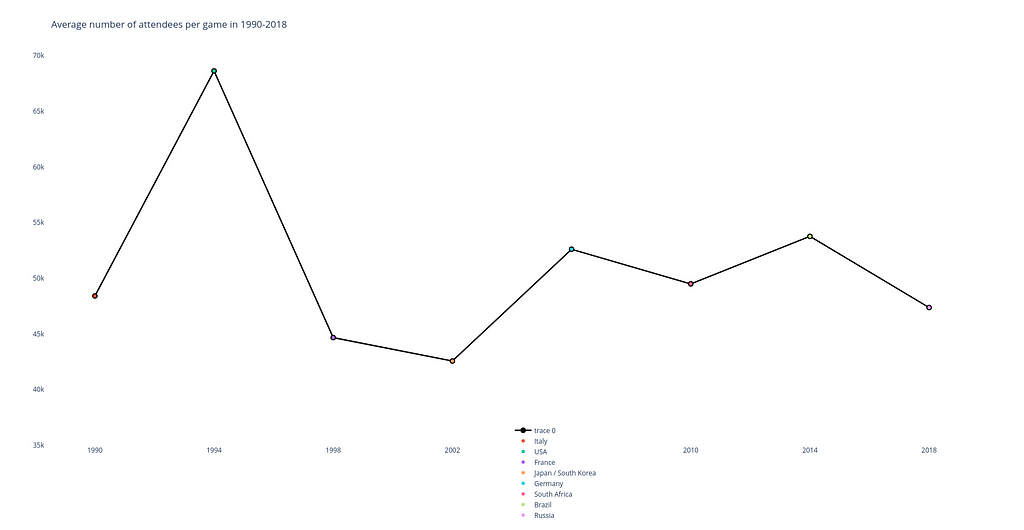
The line plot can be a wise choice for displaying the dynamics of changing our data with time. In the case below we will combine a line plot with a scatter plot to mark each location with its own color.
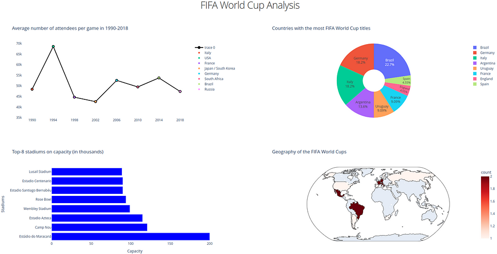
Below you can find a code snippet using Plotly that produces a line chart showing the average attendance at the FIFA World Cup over the period 1990–2018: each value is marked with a label and a colored scatter point.
# Line plot fig.add_trace(go.Scatter(x=time, y=numbers, mode='lines+markers', marker=dict(color='black',size=10), line=dict(width=2.5)))
# Scatter plot for i in range(len(time)): fig.add_trace(go.Scatter(x=[time[i]], y=[numbers[i]], mode='markers', name=labels[i]))
# Layout settings fig.update_layout(title='Average number of attendees per game in 1990-2018', xaxis=dict(tickvals=time), yaxis=dict(range=[35000, 70000]), showlegend=True, legend=dict(x=0.5, y=-0.2), plot_bgcolor='white')
fig.show()
And the result looks as follows:
Line plot built with Plotly. Image by Author.
When you hover your mouse over any point of the chart in Plotly, a window pops up showing the number of spectators and the name of the country where the tournament was held.
Level of similarity to Matplotlib plot: 8 out of 10. In general, the code looks very similar to the initial snippet in terms of structure and the placement of the main code blocks inside it.
What is different: However, some differences are also presented. For instance, pay attention to details how plot elements are declared (e.g. a line plot mode lines+markers which allows to display them simultaneously).
What is important: For building this plot I use the plotly.graph_objects (which is imported as go) module. It provides an automatically-generated hierarchy of classes called ‘graph objects’ that may be used to represent various figures.
#2. Pie Chart (actually, a donut chart)
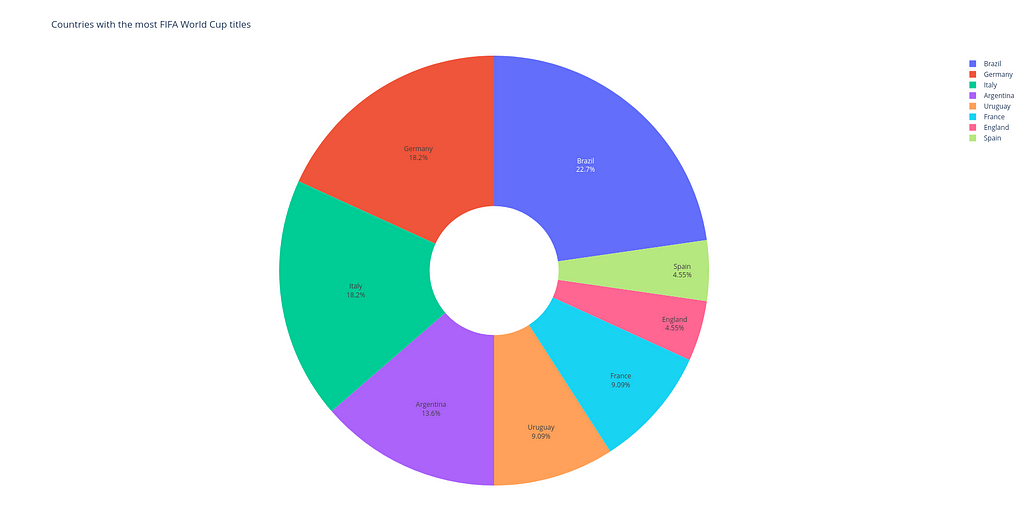
Pie & donut charts are very good for demonstrating the contributions of different values to a total amount: they are divided in segments, which show the proportional value of each piece of our data.
Here is a code snippet in Plotly that is used to build a pie chart which would display the proportion between the countries with the most World Cup titles.
# Building chart fig = px.pie(values=freq, names=label_list, title='Countries with the most FIFA World Cup titles', color_discrete_map=dict(zip(label_list, colors)), labels={'label': 'Country', 'value': 'Frequency'}, hole=0.3)
The resulting visual item is given below (by the way, it is an interactive chart too!):
Pie chart built with Plotly. Image by Author.
Level of similarity to Matplotlib plot: 7 out of 10. Again the code logic is almost the same for the two versions.
What is different: One might notice that with a help of hole keyword it is possible to turn a pie chart into a donut chart. And see how easy and simple it is to display percentages for each segment of the chart in Plotly compared to Matplotlib.
What is important: Instead of using plotly.graph_objects module, here I apply plotly.express module (usually imported as px) containing functions that can create entire figures at once. This is the easy-to-use Plotly interface, which operates on a variety of types of data.
#3. Bar Chart
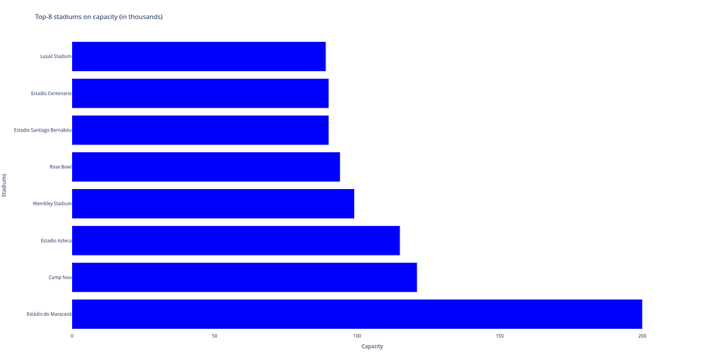
Bar charts, no matter whether they are vertical or horizontal, show comparisons among different categories. The vertical axis (‘Stadium’) of the chart shows the specific categories being compared, and the horizontal axis represents a measured value, i.e. the ‘Capacity’itself.
# Horizontal bar chart fig.add_trace(go.Bar(y=labels, x=capacity, orientation='h', marker_color='blue'))
# Layout settings fig.update_layout(title='Top-8 stadiums on capacity (in thousands)', yaxis=dict(title='Stadiums'), xaxis=dict(title='Capacity'), showlegend=False, plot_bgcolor='white')
fig.show()
Horizontal bar chart built with Plotly. Image by Author.
Level of similarity to Matplotlib plot: 6 out of 10. All in all, the two code pieces have more or less the same blocks, but the code in Plotly is shorter.
What is different: The code fragment in Plotly is shorter because we don’t have to include a paragraph to place labels for each column — Plotly does this automatically thanks to its interactivity.
What is important: For building this type of plot, plotly.express module was also used. For a horizontal bar char, we can use the px.bar function with orientation=’h’.
#4. Choropleth Map
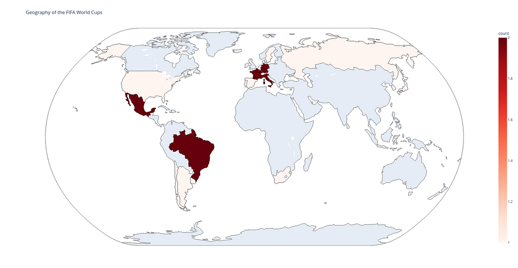
Choropleth map is a great tool for visualizing how a variable varies across a geographic area. A heat map is similar, but uses regions drawn according to a variable’s pattern rather than geographic areas as choropleth maps do.
Below you can see the Plotly code to draw the chorogram. Here each country gets its color depending on the frequency how often it holds the FIFA World Cup. Dark red countries hosted the tournament 2 times, light red countries — 1, and all others (gray) — 0.
## Choropleth Map ##

import polars as pl
import plotly.express as px

df = pl.read_csv('data_football.csv')
df.head(5)
fig = px.choropleth(df, locations='team_code', color='count',
                    hover_name='team_name', projection='natural earth',
                    title='Geography of the FIFA World Cups',
                    color_continuous_scale='Reds')
fig.show()
Choropleth map built with Plotly. Image by Author.
Level of similarity to Matplotlib plot: 4 out of 10. The code in Plotly is three times smaller than the code in Matplotlib.
What is different: While using Matplotlib to build a choropleth map, we have to do a lot of additional staff, e.g.:
to download a zip-folder ne_110m_admin_0_countries.zip with shapefiles to draw the map itself and to draw country boundaries, grid lines, etc.;
to import Basemap, Polygon and PatchCollection items from mpl_toolkits.basemap and matplotlib.patches and matplotlib.collections libraries and to use them to make colored background based on the logic we suggested in data_football.csv file.
What is important: And what is the Plotly do? It takes the same data_football.csv file and with a help of the px.choropleth function displays data that is aggregated across different map regions or countries. Each of them is colored according to the value of a specific information given, in our case this is the count variable in the input file.
As you can see, all Plotly codes are shorter (or the same in a case of building the line plot) than those in Matplotlib. This is achieved because Plotly makes it far easy to create complex plots. Plotly is great for creating interactive visualizations with just a few lines of code.
Sum Up: Creating a Single Dashboard with Dash
Dash allows to build an interactive dashboard on a base of Python code with no need to learn complex JavaScript frameworks like React.js.
Here you can find the code and comments to its important parts:
import polars as pl import plotly.express as px import plotly.graph_objects as go import dash from dash import dcc from dash import html
for i in range(len(time)): chart1.add_trace(go.Scatter(x=[time[i]], y=[numbers[i]], mode='markers', name=labels[i]))
# Layout settings chart1.update_layout(title='Average number of attendees per game in 1990-2018', xaxis=dict(tickvals=time), yaxis=dict(range=[35000, 70000]), showlegend=True, plot_bgcolor='white')
# Building chart chart2 = px.pie(values=freq, names=label_list, title='Countries with the most FIFA World Cup titles', color_discrete_map=dict(zip(label_list, colors)), labels={'label': 'Country', 'value': 'Frequency'}, hole=0.3)
# Building chart chart4 = px.choropleth(df, locations='team_code', color='count', hover_name='team_name', projection='natural earth', title='Geography of the FIFA World Cups', color_continuous_scale='Reds')
if __name__ == "__main__": app.run_server(debug=False)
Comments to the code:
First, we need to import all libraries (including HTML modules) and initialize dashboard with a help of the string app = dash.Dash(__name__, external_stylesheets=external_stylesheets).
We then paste each graph into Dash core components to further integrate them with other HTML components (dcc.Graph). Here className=”six columns” needs to use half the screen for each row of plots.
After that we create 2 rows of html.Div components with 2 plots in each. In addition, a simple CSS with the style attribute can be used to display the header of our dashboard in the layout string. This layout is set as the layout of the app initialized before.
Finally, the last paragraph allows to run the app locally (app.run_server(debug=False)). To see the dashboard, just follow the link http://127.0.0.1:8050/ and you will find something like the image below.
The final dashboard built with Dash. Image by Author.
Final Remarks
Honestly, the question in the title was rhetorical, and only you, dear reader, can decide whether the current version of the dashboard is better than the previous one. But at least I tried my best (and deep inside I believe that version 2.0 is better) 🙂
You may think that this post doesn’t contain any new information, but I couldn’t disagree more. By writing this post, I wanted to emphasize the importance of improving skills over time, even if the first version of the code may not look that bad.
I hope this post encourages you to look at your finished projects and try to remake them using the new techniques available. That is the main reason why I decided to substitute Matplotlib with Plotly & Dash(plus the latter two make it easy to create data analysis results).
The ability to constantly improve your work by improving an old version or using new libraries instead of the ones you used before is a great skill for any programmer. If you take this advice as a habit, you will see progress, because only practice makes perfect.
Strategically enhancing address mapping during data integration using geocoding and string matching
Many individuals in the big data industry may encounter the following scenario: Is the acronym “TIL” equivalent to the phrase “Today I learned” when extracting these two entries from distinct systems? Your program might get confused too when records come in with different names even though it means the same thing. As we are pulling data with discrepancies together from different operational systems, the data ingestion process can be more time-consuming than originally thought!
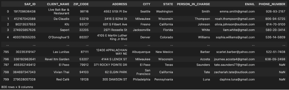
Now, you are working for a food supply chain company whose clients are from the catering industry. The company provides two data extracts about clients’ contact information and their restaurant details from different operational systems. You need to link them together so that the front-end dashboarding team can gain more information from the populated data. Unfortunately, there are no unique primary keys to link these two data sources but some geographic information and names of restaurants. This article is going to enhance your geographical mapping solution by combining geopy and fuzzywuzzy on top of manual mapping.
Using pandas read the two data sources:
Image by the author: custom_master.csvImage by the author: client_profile.csv
Basic Data Cleaning and Manual Mapping
When dealing with large datasets, every factor that might affect the accuracy of mapping needs to be considered. Including basic data cleaning and manual mapping as the first step can improve data consistency and alignment for more accurate results.
*The following code should be applied to both data sources.
1: Capitalization (eg. 123 Main St and 123 MAIN ST should be mapped)
2: Inadvertent Whitespace and Unnecessary Punctuations (eg. 123 Main St_whitespace_ or 123 Main St; should be mapped with 123 Main St)
3: Standardizing Postal Abbreviation (eg. 123 Main Street should be mapped with 123 Main St)
Please consider using the full standardized postal abbreviation mapping table from the United States Postal Service Street Suffix Abbreviationsin practical applications for higher consistency and accuracy in mapping geographical locations.
Other potential factors that might affect the accuracy of mapping include misspellings in addresses (eg. 123 Mian St and 123 Main St) and shortened addresses (eg. 123 Forest Hill and 123 Frst Hl) could be challenging to tackle using manual mapping approach, which more advanced mapping technique should be introduced.
Geopy
Geopy is an open-source Python library that plays a crucial role in the geospatial landscape by converting human-readable addresses into precise geographic coordinates through address geocoding. It employs great-circle distance calculations to accurately compute latitude and longitude during the geocoding process. Other geocoding APIs such as the Google Maps Geocoding API, OpenCage Geocoding API, and Smarty API can also be considered based on the specific business requirements of the project.
After the geocoding process, we can merge the two DataFrames using LATITUDE and LONGITUDE columns with pandas library and check the number of rows that are successfully mapped. Addresses that cannot be mapped will be passed on to the next mapping stage.
Fuzzy Wuzzy
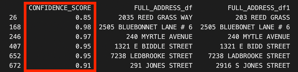
Fuzzywuzzy is another Python library that is designed to facilitate fuzzy string matching, by providing a set of tools for comparing and measuring the similarity between strings. The library uses algorithms like Levenshtein distance to quantify the degree of resemblance between strings, which is particularly useful for data containing typos or discrepancies. A confidence score will be populated for each address comparison, which is a numerical value between 0 and 100. A higher score suggests a stronger similarity between the strings, while a lower score indicates a lesser degree of similarity. In our case, we can use fuzzywuzzy to tackle the remaining rows that cannot be mapped with geopy.
Image by the author: Output from the code above using fuzzywuzzy to show confidence_score for the remaining rows that were unmapped.
The demo above only uses column ADDRESS for string matching, adding another column in common CLENT_NAME to this process can advance mapping in this business scenario which brings more accurate output.
Conclusion
This address mapping technique is versatile across various industries. The combination of manual mapping, geopy, and fuzzywuzzy provides a comprehensive approach to enhance geographical mapping accuracy, making it a valuable asset for businesses across different sectors that a facing similar challenges in data ingestion and integration.
As the AI Act was officially adopted in late January, I’ve gotten tangled up in a couple of its provisions. Some of them regulating emotion recognition technologies, which got me admittedly more tangled up than I originally anticipated. Maybe I was just looking for an excuse for getting back into researching some of my personally favourite topics: human psyche, motivation and manipulation. In any event, I discovered many new and interesting technologies, but was disappointed to find much less exciting legal analyses of the questions they raise. As the hamster wheel in my head continued spinning, I couldn’t help myself but writing some of the things down.
The series Emotions-in-the-loop is planned in the following way: I will first set up the scene imagining a hypothetical (although to a greater degree already possible) scenario of a morning in the life of (scanned) Jane. Then, I will describe the technologies that could be used to make this hypothetical scenario a reality, together with referencing patents and papers justifying my claim that we are already at the point where Scanned Jane could exist somewhere out there. The point of this first part will be to demonstrate just how far the technologies can go and to hopefully make the readers wonder at which point the scenario goes from a utopia to a dystopia. At least for them personally.
In the following sequels, I will then analyze the legal situation of the fictitious scenario. Hopefully helping demonstrate where some of the gaps in protecting individuals persist in our legal frameworks. I will do that by focusing on the protection provided (or lack thereof) by the GDPR, the recently adopted Data Act, and the upcoming AI Act. The point being: these regulations fail miserably at protecting individuals from some of the (potentially) most useful and at the same time most easily misused technologies available nowadays. Especially when these are combined as in the imagined (admittedly slightly Black-Mirror-like) scenario.
As I’m developing the idea of the series on the go, I have no clue where exactly it might take me. Still, if you are also up for some dangerous speculations paired with far-fetched claims and some legal analysis sprinkled on top, hop on and enjoy the ride!
Painting the Picture: A Morning in the Life of (Scanned) Jane
Jane opens her eyes. It takes a second or two for her to figure out where she is. Oh good, it’s her room.
(What day is it, do I even have to get up?)
Her hand stretches out to the side cupboard, she feels her glasses and puts them on her head.
— Good morning, Jane! — a soft female voice says.
— Looks like you didn’t sleep that well. — the voice continues — You should probably consider buying a new ergonomic mattress. I found 12 online that would be perfect for you. I can set a reminder for you to check them out. Or should I just order the one with the best price/quality ratio based on user reviews? — the voice stops.
— Just order it — Jane hears herself mumbling the words before she could even think them through. (It is so early after all. Or is it? What day is it?)
— It’s Sunday the 12 of July 2027, 8:30 AM. It is also your mother’s birthday today, I bought her the antique Chinese vase you wanted. — short pause — You should leave the house by 12, so you make it in time. The weather will be sunny and warm.
— Oh right — Jane thinks to herself. — Yes thanks, I’ll get up now.
(Hmm.. I guess I do feel a bit tired. It’s a good thing I’m ordering the new mattress, I probably need it. Wait, I can’t remember picking any vase for my mom?)
— Is everything alright, you look worried? — the voice again.
— Oh yes, I was just wondering about the vase. I can’t remember choosing it.
— You didn’t, you were busy with work so I picked one for you.
(Oh right, yes, now I remember.)
— Your coffee is waiting for you in the kitchen. I’ll put some upbeat music on, it might help you get up and get into a cheerful mood for the birthday party.
— Great thank you. — Jane slowly makes her way to the kitchen.
(Where did I leave my phone?)
— Your phone is in the bathroom, you left it there yesterday evening while taking a shower and didn’t take it with you when you went to bed.
— Right…. — Jane makes her way to the bathroom, takes her phone, and opens the analytics app.
(Interesting.)
Her app shows that she had multiple pulse increases during the night, and moved a lot.
— Yes, you had a pretty rough night — the voice continues, this time in a slightly worried tone — you should probably consider seeing a physician. I looked up your symptoms and certain non-prescription medications might help as well. Do you want me to order them?
Jane is now starting to feel slightly worried herself.
— Well, I don’t know… Is it serious, should I really go see a physician?
— I can order the medication and save the list of physicians in case you continue sleeping poorly. Is that okay?
— Yes, I guess that sounds reasonable.
— Great, the medication is on its way and will arrive here tomorrow. Now you can relax and drink your coffee. I have also prepared a list of news that might interest you and the taxi will be here to drive you to your mother’s at exactly 15 to 12.
(Perfect!)
Jane makes her way to her coffee. God knows she needs it. A couple of seconds later Jane is surprised to find her favorite coffee cup only halfway full.
— Hey Lucy, why is my cup only halfway full?
— Well — the voice starts carefully — you locked the settings yesterday to halve the amount of coffee you drink per day. You said it makes you jittery.
(Did I? Oh right…Well okay, I guess that is the right call.)
Jane opens the fridge and is again surprised to find no milk in it. Now already annoyed Jane proceeds:
— Why is there no milk in the fridge?
— Well you also said that you will only drink black coffee from now on, to help you lose weight. — the voice sounds very worried now — You also said not to change these settings no matter what you tell me afterward.
Jane is now completely confused.
(Did I actually say that??)
— No, I’m pretty sure I’ve never said that.
— Sure you have! Remember two days ago when you were looking at yourself in the mirror while trying that skirt on at the shopping mall?
(Hmmm… I can’t remember saying it, but I definitely wasn’t happy with how I looked in that skirt… Maybe I did say it after all? Well, it’s probably for the better, I should really lose some weight before the summer. But oh I really need another cup of coffee…)
— In case you are still feeling tired after your coffee, I also ordered the Feel Good pill to help energize you without making you jittery. They are in the cupboard next to the fridge.
— Wow, sometimes it’s like you can read my mind!
— I’m happy to be of assistance, let me know if there is anything else I can help you with!
Jane is only half-listening to the voice now.
(Oh I knew that getting this smart analytics package was a good idea!)
[Jane never said that she didn’t want to drink coffee with milk anymore or that she wanted to halve her caffeine intake. She did, however, feel terribly distressed at the store the other day and said to her friend on the same day that she needed to lose weight ASAP and should probably stop “drinking her calories”. She does have trouble sleeping as well, which is only made worse by the high caffeine intake. What else was Lucy supposed to do?]
Where Sci-Fi Meets Reality
The particular point where the previously described scenario becomes less appealing and more worrying will heavily differ from one person to the other. While some will be more than happy to leave the all too many little everyday decisions to the algorithms, others might wonder about the loss of control and dehumanizing effect that the described scenario might have. And when it comes to drawing lines and deciding what can or cannot and what should or should not be tolerated, the clock for making these decisions is slowly but steadily ticking.
In the hypothetical morning of our Scanned Jane and her good friend, interconnected, all-knowing AI Lucy (association with the movie is made very intentionally), it’s not at all so unimaginable that the described scenario might soon become reality. Smartwatches measuring all types of activities and processing a whole stream of bodily data (including even blood sampling) are nothing new. Nor is the possibility of connecting the collected data streams across multiple devices. (Just think about the fact that the Internet of Things (IoT) can be traced at least back to 1999.) The science behind “high-quality sleep” is also getting increasingly more predictable and therefore also adjustable. So much so that you can even connect your sensors to allow free data flows to your ‘smart mattress’ that will then adjust the temperature, firmness, and other features. Finally, all the collected data can also already help your device predict your mental and cognitive state (even more so with special smart glasses tracking your eye movements and brain waves). This then in turn makes it possible to provide recommendations as to the actions you might want to take to improve your condition, but also to help medical workers provide better treatments. From there it is basically a baby step to also connect all that useful data, combine it with the data collected by your smart glasses and have super personalized predictions and recommendations. The glasses then also allowing for a seamless user experience. Of course, all the newest smart glasses also have full internet access and their own AI-powered smart voice assistants to basically act as your consciousness. (Or maybe in place of it?) Finally, the voice assistants are then more than capable of both making decisions for you as well as executing those decisions if you give them the necessary permissions of course. And have enough confidence in their decisions. Not to mention smart fridges can already do your shopping for you, and in a way that optimizes your health and nutrition all on their own.
Our willingness to surrender to these technologies will usually depend on our affinity towards technology and the amount of control we are willing to give over. (As well as in terms of the depicted scenario, the lack of self-control to actually go through with our decisions ourselves.) I for one, am sure I’m not going to resolve to these technologies any time soon, but I’m certain some people will. And it is also my opinion that there should be something resembling a line of human dignity and freedom of choice we can never (even willfully) give away. Or should never be able to give away. This does not appear to be the dominating mindset at the moment.
So what’s the big deal?
Now, for the million-dollar question: what’s the big deal? Jane is happy with the technology and not having to worry about what day it is, what she is going to get her mother for her birthday, or how she is going to lose weight, as long as she loses it. Everyone is free to make their own choices, the technology is here to serve us, so why can’t I just let it be?
I’ve battled with similar questions a fair bit myself and the only answer I can offer rests on a couple of points, features, characteristics, facts, or whatever you want to call them.
Our environment undeniably has a great influence on us as individuals. However, in comparison to other people expressing their opinions, these technologies work invisibly. We are oftentimes not aware they are doing anything let alone that this affects us. They lock us in filter bubbles. They shape or reaffirm our beliefs. And there isn’t anything we can do about it. How do you fight something that is basically a voice in your own head?
Although some people don’t have a problem with technologies subconsciously altering their behaviour (as long as it’s changing them for the better), this is not a universal phenomenon. We should all have the right to decide how we want to shape our opinions, beliefs, and decisions, as well as be able to change our decisions later on.
These technologies raise multiple ethical questions on the side of the data processing necessary to train the algorithms, as well as the data processing necessary for them to generate their assumptions and predictions, and finally, as to the effects they may cause. These questions already justify giving the super smart watches, fridges, phones, cars, and glasses (especially when they all work together) a bit more attention. Is there a line to what people can agree to? To be more precise can I agree to an algorithm subconsciously manipulating me to eat healthier? Many would sign that pact with the devil in a heartbeat to have their smartwatch and fridge collaborate and not let them open the fridge after they “spent” all their calories for the day or the clock has ticked 8 PM. To others, this may sound like a Black Mirror episode just before the plot twist makes the useful technology fully dystopic.
Considering these new ethical dilemmas we are being confronted with, do we also need to establish new rights? Should we all have the right to lose control and go against what is good for us? To make our own decisions even if they contravene our general preferences? What if we have opposing goals? And what do we do with the commercial interests of various actors offering the technologies or relying on the data they get from the ones offering it?
What do we do with the actors, wanting to use these technologies for malevolent purposes? People have always been prone to deceit and had a weakness for using manipulation if it may help purport their agenda. Aside from the commercial interests and the “danger” of getting extra-personalized ads, what happens if these systems start being used by the state to purport an existing political system? (Hello China.) How do we fight manipulation if we don’t even know we are being manipulated in the first place? Which actor in society would we trust enough to conduct surveillance of these systems and their use?
The hypothesis of this blog series is that the current laws are insufficient to deal with many (if not all) of these questions and the novel risks they impose on individuals as well as society. The series will first try to exemplify why this is the case by comparing the scenario against the requirements of the GDPR, then the Data Act, and finally the upcoming AI Act. Hopefully, by analyzing these questions through the lens of the applicable legal framework we can identify some of the gaps and collectively think through how we can try closing them.
I wish us all good luck with it!
Emotions-in-the-loop was originally published in Towards Data Science on Medium, where people are continuing the conversation by highlighting and responding to this story.
We use cookies on our website to give you the most relevant experience by remembering your preferences and repeat visits. By clicking “Accept”, you consent to the use of ALL the cookies.
This website uses cookies to improve your experience while you navigate through the website. Out of these, the cookies that are categorized as necessary are stored on your browser as they are essential for the working of basic functionalities of the website. We also use third-party cookies that help us analyze and understand how you use this website. These cookies will be stored in your browser only with your consent. You also have the option to opt-out of these cookies. But opting out of some of these cookies may affect your browsing experience.
Necessary cookies are absolutely essential for the website to function properly. These cookies ensure basic functionalities and security features of the website, anonymously.
Cookie
Duration
Description
cookielawinfo-checkbox-analytics
11 months
This cookie is set by GDPR Cookie Consent plugin. The cookie is used to store the user consent for the cookies in the category "Analytics".
cookielawinfo-checkbox-functional
11 months
The cookie is set by GDPR cookie consent to record the user consent for the cookies in the category "Functional".
cookielawinfo-checkbox-necessary
11 months
This cookie is set by GDPR Cookie Consent plugin. The cookies is used to store the user consent for the cookies in the category "Necessary".
cookielawinfo-checkbox-others
11 months
This cookie is set by GDPR Cookie Consent plugin. The cookie is used to store the user consent for the cookies in the category "Other.
cookielawinfo-checkbox-performance
11 months
This cookie is set by GDPR Cookie Consent plugin. The cookie is used to store the user consent for the cookies in the category "Performance".
viewed_cookie_policy
11 months
The cookie is set by the GDPR Cookie Consent plugin and is used to store whether or not user has consented to the use of cookies. It does not store any personal data.
Functional cookies help to perform certain functionalities like sharing the content of the website on social media platforms, collect feedbacks, and other third-party features.
Performance cookies are used to understand and analyze the key performance indexes of the website which helps in delivering a better user experience for the visitors.
Analytical cookies are used to understand how visitors interact with the website. These cookies help provide information on metrics the number of visitors, bounce rate, traffic source, etc.
Advertisement cookies are used to provide visitors with relevant ads and marketing campaigns. These cookies track visitors across websites and collect information to provide customized ads.