Category: AI

A pragmatic guide to understand AI risks and build trust with users through responsible AI development

In the fast-paced technology landscape, product teams feel the relentless pressure to rush innovative AI offerings to market. However, prioritizing speed over ethical and safety considerations can severely backfire. When AI systems breach social norms and values, organizations bear the risk of facing long-lasting reputational damage and losing trust with users.

Companies are caught in a real-world “prisoner’s dilemma” of the AI era — while collective adherence to ethical development is ideal, it’s often more tempting for companies to secure a first-mover advantage by compromising on these crucial standards. This tension is exemplified by the infamous Facebook-Cambridge Analytica scandal, where taking ethical shortcuts led to grave, long-lasting reputational damage. As AI becomes more entrenched in our daily lives, the stakes of this ethical gamble only heightens, with each player in the industry weighing immediate gains against the longer-term value of trust and responsibility.

With the rise in AI adoption across industries since 2018, high-profile incidents of ethical violations have sharply increased. Mapping out these risks and mitigation strategies is now pivotal. This article probes the key source of AI risks, examines a few high-profile fallouts, and lays out a 6 steps framework for building products that counter these threats.

Identifying the Risks of AI

1. Privacy Intrusion & Consent Issue

Risk: Arguably the most prevalent AI pitfall is the infringement of privacy and copyright laws. This entails two distinct types of failures: failure to secure consent for the use of data, and using the data for purposes beyond the scope for which the consent was given.

Example: Artists and writers have filed class action lawsuits against OpenAI and MidJourney for training models with their work without consent. Similarly, Getty Images is suing Stability AI for using its data for model training. Privacy breaches can also occur even when consent is given but the data is used for unintended purposes. For example, Google DeepMind used the data of 1.6 million patients at the Royal London NHS Foundation Trust to build a new healthcare application. Although there was an implied consent that the data could be used to improve patients’ health, the Trust and DeepMind did not clearly communicate to patients that their information is being used to build an app.

• Artists take new shot at Stability, Midjourney in updated copyright lawsuit
• Why Google consuming DeepMind Health is scaring privacy experts

2. Algorithmic Bias

Risk: This risk involves AI systems making biased predictions, which systematically disadvantages or excludes certain group of people based on characteristics like race, gender, or socio-economic background. Such biases can have significant societal impact, especially when the AI is used to make critical decisions impacting the lives of the individuals.

Example: There was backlash against Apple in 2019, when allegations surfaced that men received higher credit limits for Apple Credit Cards than women, despite women having better credit scores in some cases. Other notable instances include AI-driven recruitment software and criminal justice applications, such as the COMPAS tool, which have been criticized for displaying racial and gender bias.

• Apple Card is accused of gender bias. Here’s how that can happen | CNN Business
• Opinion | When an Algorithm Helps Send You to Prison (Published 2017)

3. Accuracy Risk & Explainability Gap

Risk: Significant risks arise when AI systems that are used for making high-stakes decisions provide inaccurate results or fail to offer a clear rationale for their output. The ‘black box’ nature of the AI makes it difficult for users to understand and verify its results, which obscures accountability and leads to a loss of trust.

Example: IBM Watson for Oncology was designed to provide clinicians with personalized recommendations for cancer treatment. However, reports surfaced that Watson gave unsafe and incorrect treatment suggestions, which led to a loss of trust in technology and damaged IBM’s reputation.

IBM’s Watson supercomputer recommended ‘unsafe and incorrect’ cancer treatments, internal documents show

4. Security Risk

Risk: A significant societal risks emerge from the use of AI to create deepfakes, which involves generating highly convincing images or video that makes it appear as though individuals are saying or doing things they never actually did. Deepfakes have been used to create deceptive and realistic media that can be used for committing fraud, spreading misinformation, or damaging reputations. Moreover, AI can be weaponized for cyberattacks and social engineering, like tailoring phishing campaigns, which can introduce extensive security vulnerabilities.

Example: In the political domain, use of deepfakes to fabricate speeches or actions could sway public opinion during critical events like elections. During the Russia-Ukraine conflict, a deepfake showing Ukrainian president appearing to tell his soldiers to lay down arms and surrender was circulated, an act that could have demoralized troops and provided time-sensitive tactical advantage to Russia. In the cybersecurity realm, AI-powered voice imitation was used to impersonate a CEO’s voice convincingly, leading to a fraudulent transfer of funds.

• Deepfake video of Zelenskyy could be ‘tip of the iceberg’ in info war, experts warn
• Unusual CEO Fraud via Deepfake Audio Steals US$243,000 From UK Company

6 Step Framework for Mitigating AI Risks

Managing AI risks requires a thoughtful approach throughout the entire product life-cycle. Below is a six step framework, organized by different stages of AI development, that organizations can adopt to ensure the responsible use of AI technology in their products.

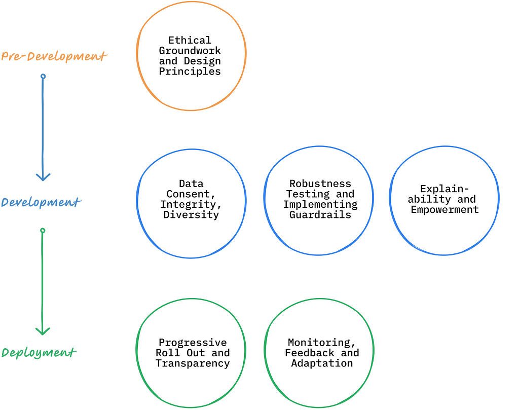
1. Pre-Development: Ethical Groundwork and Design Principles

Before a single line of code is written, product teams should lay out the groundwork. Prioritize early engagement with a broad set of stakeholders, including users, technical experts, ethicists, legal professionals, and members of communities who may be impacted by the AI application. The goal is to identify both the overt and subtle risks associated with the product’s use case. Use these insights to chalk out the set of ethical guidelines and product capabilities that needs to be embedded into the product prior to its launch to preemptively address the identified risks.

2. Development: Data Consent, Integrity, Diversity

Data is the bedrock of AI and also the most significant source of AI risks. It is critical to ensure that all data procured for model training are ethically sourced and comes with consent for its intended use. For example, Adobe trained its image generation model (Firefly) with proprietary data which allows it to provide legal protection to users against copyright lawsuits.

Further, Personally Identifiable Information (PII) should be removed from sensitive datasets used for training models to prevent potential harm. Access to such datasets should be appropriately gated and tracked to protect privacy. It’s equally important to ensure that the datasets represent the diversity of user base and the breadth of usage scenarios to mitigate bias and fairness risks. Companies like Runway have trained their text-to-image models with synthetic datasets containing AI-generated images of people from different ethnicities, genders, professions, and ages to ensure that their AI models exhibit diversity in the content they create.

• How Adobe’s Copyright Protection Will Make it an AI Leader
• Mitigating stereotypical biases in text to image generative systems | Runway Research

3. Development: Robustness Testing and Implementing Guardrails

The testing phase is pivotal in determining AI’s readiness for a public release. This involves comparing AI’s output against the curated set of verified results. An effective testing uses:

• Performance Metrics aligned with user objectives and business values,
• Evaluation Data representing users from different demographics and covering a range of usage scenarios, including edge-cases

In addition to performance testing, it is also critical to implement guardrails that prevents AI from producing harmful results. For instance, ImageFX, Google’s Image generation service, proactively blocks users from generating content that could be deemed inappropriate or used to spread misinformation. Similarly, Anthropic has proactively set guardrails and measures to avoid misuse of its AI services in 2024 elections.

• New and better ways to create images with Imagen 2
• Anthropic on LinkedIn: Preparing for global elections in 2024

4. Development: Explainability & Empowerment

In critical industry use cases where building trust is pivotal, it’s important for the AI to enable humans in an assistive role. This can be achieved by:

• Providing citations for the sources of the AI’s insights.
• Highlighting the uncertainty or confidence-level of the AI’s prediction.
• Offering users the option to opt-out of using the AI.
• Creating application workflows that ensure human oversight and prevent some tasks from being fully automated.

5. Deployment: Progressive Roll Out & Transparency

As you transition the AI systems from development to real-world deployment, adopting a phased roll-out strategy is crucial for assessing risks and gathering feedback in a controlled setting. It’s also important to clearly communicate the AI’s intended use case, capabilities, and limitations to users and stakeholders. Transparency at this stage helps manage expectations and mitigates reputational risks associated with unexpected failures of the AI system.

OpenAI, for example, demonstrated this approach with Sora, its latest text-to-video service, by initially making the service available to only a select group of red teamers and creative professionals. It has been upfront about Sora’s capabilities as well as its current limitations, such as challenges in generating video involving complex physical interactions. This level of disclosure ensures users understand where the technology excels and where it might fail, thereby managing expectations, earning users’ trust, and facilitating responsible adoption of the AI technology.

Sora: Creating video from text

6. Deployment: Monitoring, Feedback, and Adaptation

After an AI system goes live, the work isn’t over. Now comes the task of keeping a close watch on how the AI behaves in the wild and tuning it based on what you find. Create an ongoing mechanism to track performance drifts and continually test and train the model on fresh data to avoid degradation in the AI performance. Make it easy for users to flag issues and use these insights to adapt AI and constantly update guardrails to meet high ethical standards. This will ensure that the AI systems remain reliable, trustworthy, and in step with the dynamic world they operate in.

Conclusion:

As AI becomes further entrenched in our lives, managing ethical risks proactively is no longer optional — it is imperative. By embedding ethical considerations in every step of bringing AI products to life, companies not only mitigate risks but also build foundational trust with their users. The era of “move fast and break things” cannot be applied when dealing with technologies that are exponentially more powerful than anything we have seen before. There are no shortcuts when it comes to managing risks that can have far-reaching societal impacts.

AI product builders have a duty to society to move more intentionally and purposefully, making trust their true North Star. The future success and continued progress of AI hinges on getting the ethics right today.

Thanks for reading! If these insights resonate with you or spark new thoughts, let’s continue the conversation. Share your perspectives in the comments below or connect with me on LinkedIn.

---

6 Step Framework to Manage Ethical Risks of Generative AI in Your Product was originally published in Towards Data Science on Medium, where people are continuing the conversation by highlighting and responding to this story.

A post on creating a custom IPython Jupyter Magic command

Introduction

Jupyter Notebooks are commonplace in data science. They allow a mixture of “repeat, evaluation, loop” (REPL) code writing and documentation in a single place. They’re most commonly used for analysis and brainstorming purposes, but also, more contentiously, some prefer notebooks to scripts to run production code (but we won’t focus on that here).

Invariably, the code written in notebooks will be repetitive in some way such as setting up a database connection, displaying an output, saving results, interacting with an internal platform tool, etc. It’s best to store this code as functions and/or modules to make them reusable and more easily manage them.

However, the notebook experience is not always improved when you do that. For instance, you still need to import and call these functions throughout your notebook, which doesn’t change the notebook experience much at all. So what is the answer to augmenting the notebook development experience itself? IPython Jupyter Magic Commands.

IPython Jupyter Magic commands (e.g. lines in notebook cells starting with % or %%) can decorate a notebook cell, or line, to modify its behavior. Many are available by default, including %timeit to measure the execution time of the cell and %bash to execute shell commands, and others are provided by extensions such as %sql to write SQL queries directly in a cell of your notebook.

In this post, we’ll show how your team can turn any utility function(s) into reusable IPython Jupyter magics for a better notebook experience. As an example, we’ll use Hamilton, an open source library we created, to motivate the creation of a magic that facilitates better development ergonomics for using it. You needn’t know what Hamilton is to understand this post.

Note. Nowadays, there are many flavors of notebooks (Jupyter, VSCode, Databricks, etc.), but they’re all built on top of IPython. Therefore, the Magics developed should be reusable across environments.

Understanding IPython Jupyter Magics

IPython Jupyter Magics (which we’ll shorten to just Magics) are bits of code that can be dynamically loaded into your notebooks. They come in two flavors, line and cell magics.

Line magic, as it suggests, operates on a single line. That is, it only takes in as input what is specified on the same line. They are denoted by a single % in front of the command.

# will only time the first line
%time print("hello")
print("world")

Cell magic, as it suggests, takes the entire contents of a cell. They are denoted by a double `%%`in front of the command.

# will time the entire cell
%%timeit
print("hello")
print("world")

Jupyter comes with several in-built magic commands. You can think of them as “command line” tools that have access to the entire notebook context. This allows them to interact with the notebook output (e.g., printing results, displaying a PNG, rendering HTML), but also to modify the state of existing variables and write to other code and markdown cells!

This is great for developing internal tooling because it can abstract away and hide from the user unnecessary complexities, making the experience “magical”. This is a powerful tool to develop your own “platform efforts”, especially for MLOps and LLMOps purposes, as you can hide what is being integrated with from having to be exposed in the notebook. It therefore also means that notebooks don’t need to be updated if this abstracted code changes under-the-hood, since it can all be hidden in a python dependency upgrade.

Workflow example

Magic commands have the potential to make your workflow simpler and faster. For example, if you prefer to develop in a notebook before moving your code to a Python module, this can involve error-prone cutting & pasting. For this purpose, the magic %%writefile my_module.py will directly create a file and copy your cell content into it.

On the opposite hand, you might prefer developing in my_module.py in your IDE and then load it into a notebook to test your functions. This usually involves restarting the notebook kernel to refresh the module imports, which can be tedious. In that case, %autoreload will automatically reload every module imports before every cell execution, removing this friction point!

The Need for Custom Magic Commands

In the post How well-structured should your data code be?, it is argued that standardization/centralization/“platform” efforts, should change the shape of the “move quickly vs. built-to-last” trade-off curve for the better. A concrete tactic to change this trade-off is to implement better tooling. Better tooling should make what used to be complex, simpler and accessible. Which is exactly what you can achieve with your own custom Magic commands, which translates to less of a trade-off to be made.

A Hamilton Magic Command

For those unfamiliar with Hamilton we point readers to the many TDS articles with it (e.g. origin story, Production prompt engineering, Simplifying Airflow DAG Creation & Maintenance, Tidy Production Pandas, etc.) as well as https://www.tryhamilton.dev/.

Hamilton is an open source tool that we created at Stitch Fix back in 2019. Hamilton helps data scientists and engineers define testable, modular, self-documenting dataflows, that encode lineage and metadata. Hamilton achieves these traits in part by requiring Python functions to be curated into modules.

Nonetheless, the typical Jupyter notebook usage pattern leads to code residing in the notebook and nowhere else posing a developer ergonomics challenge:

How can we enable someone to create Python modules easily and quickly from a notebook, while also improving the development experience?

The Hamilton developer loop looks like the following:

Take a minute to read this loop. The loop shows that anytime a code change is made, the user would need to not only re-import the Python module, but also recreate the Driver object as well. Since notebooks allow cell execution in any order, it can become difficult for the user to track which version is loaded for each module and what is currently loaded in a Driver. This burden lies on the user and might require restarting the kernel, which would lose other computations (thankfully, Hamilton can be set up to execute complex dataflows and resume where you left-off…), which is less than ideal.

Here’s how we could improve this loop using Magics:

1. Create a “temporary” Python module from the functions defined in a cell, and import this new module directly in the notebook.
2. Automatically visualize the directed acyclic graph (DAG) defined by the functions to reduce visualization boilerplate code.
3. Rebuild all Hamilton Drivers found in the notebook with updated modules, saving the user time to have to remember to manually recreate drivers to pick up the change.

What we’re going to implement

We would like a command that looks like this:

%%cell_to_module -m my_module --display --rebuild-drivers

def my_func(some_input: str) -> str:
  """Some logic"""
  return ...

And cause the following behavior after running the cell:

• Create a module with the name my_module in the notebook.
• Display the DAG constructed by the functions within the cell.
• Rebuild any downstream drivers that used my_module in other cells, saving the user having to re-run those cells.

As you can see this is a non-trivial Magic command, since we’re adjusting output of the cell and state of the notebook.

Building a Custom Magic Command

Here we lay out step by step how to create a Magic Command. To avoid only showing a trivial “hello world” example, we’ll explain how we built Hamilton’s %%cell_to_module magic as well.

Step 1: Setting up your code

Create a new Python module where we’ll write the magic code and a jupyter notebook to try it. The name of this module (i.e., `.py` file) will be the name of the extension you’ll need to load.

If Jupyter notebook is installed, you have all the required Python dependencies already. Then, add libraries you will need for your Magic, in our case Hamilton (`pip install sf-hamilton[visualization]`).

Step 2: Define your Magic Command

To define a simple Magic command, you can use functions or objects (see these docs). For more complex Magics where state is needed, you will need the class approach. We’ll use the class based approach here. To start we need to import IPython modules/functions and then define a class that inherits magic.Magics. Each method decorated with @cell_magic or @line_magic defines a new magic, and the class can house however many of them.

To start, your code should look like this at a high level:

# my_magic.py

from IPython.core import magic
from IPython.core.magic_arguments import argument, magic_arguments, parse_argstring
@magic.magics_class
class MyMagic(magic.Magics):
   """Custom class you write"""
   @magic_arguments() # needs to be on top to enable parsing
   @argument(...)   
   @magic.cell_magic
   def a_cell_magic_command(self, line, cell):
      ...
   @magic_arguments() # needs to be on top to enable parsing
   @argument(...)   
   @magic.line_magic
   def a_line_magic_command(self, line):
     ...

For stateful magic, it can be useful to add an __init__() method (i.e. constructor). It is not needed in our case.

By inheriting from `magic.Magics`, this class has access to several important fields including self.shell, which is the IPython InteractiveShell that underlies the notebook. Using it allows you to pull and introspect variables loaded in the active Jupyter notebook.

Our Hamilton Magic Command will start off looking like:

from IPython.core import magic
from IPython.core.magic_arguments import argument, magic_arguments, parse_argstring

@magic.magics_class
class HamiltonMagics(magic.Magics):
    """Magics to facilitate Hamilton development in Jupyter notebooks"""
  @magic_arguments()  # needed on top to enable parsing
  @arguments(...)
  @magics.cell_magic
  def cell_to_module(self, line, cell):
    ...

Step 3: Parsing input arguments

Next, we specify what arguments will be passed and how to parse them. For each argument, add a @argument, and add a @magic_arguments() decorator on top. They follow a similar pattern to argparse arguments if you’re familiar, but they aren’t quite as fully featured. Within the function, you need to call the parse_argstring() function. It receives the function itself to read instructions from the decorators, and `line` (the one with % or %%) which contains the arguments values.

Our command would start to look like this:

@magic_arguments() # needs to be on top to enable parsing
# flag, long form, default value, help string.
@argument("-a", "--argument", default="some_value", help="Some optional line argument")   
@magic.cell_magic
def a_cell_magic_command(self, line, cell):
   args = parse_argstring(self.a_cell_magic_command, line)
   if args.argument:
      # do stuff -- place your utility functions here

Note, for required arguments, there is no facility in magic_arguments() for that, so you need to manually check in the body of the function for correctness, etc.

Continuing our dissection of the Hamilton Magic example, the method on the class now looks like the following; we use many optional arguments:

@magic_arguments()  # needed on top to enable parsing
@argument(
    "-m", "--module_name", help="Module name to provide. Default is jupyter_module."
)  # keyword / optional arg
@argument(
    "-c", "--config", help="JSON config, or variable name containing config to use."
)  # keyword / optional arg
@argument(
    "-r", "--rebuild-drivers", action="store_true", help="Flag to rebuild drivers"
)  # Flag / optional arg
@argument(
    "-d", "--display", action="store_true", help="Flag to visualize dataflow."
)  # Flag / optional arg
@argument(
    "-v", "--verbosity", type=int, default=1, help="0 to hide. 1 is normal, default"
)  # keyword / optional arg
@magics.cell_magic
def cell_to_module(self, line, cell):
    """Execute the cell and dynamically create a Python module from its content.

     A Hamilton Driver is automatically instantiated with that module for variable `{MODULE_NAME}_dr`.
        > %%cell_to_module -m MODULE_NAME --display --rebuild-drivers
    Type in ?%%cell_to_module to see the arugments to this magic.
    """
    # specify how to parse by passing 
    args = parse_argstring(self.cell_to_module, line)  
    # now use args for logic ...

Note, the extra arguments to @argument are useful for when someone uses ? to query what the magic does. I.e. ?%%cell_to_module will show documentation.

Step 4: Implement the Command’s Logic

Now that we have parsed the arguments, we can implement the logic of the magic command. There aren’t any particular constraints here and you can write any Python code. Skipping a generic example (you have enough to get started from the prior step), let’s dig into our Hamilton Magic example. For it, we want to use the arguments to determine the desired behavior for the command:

1. Create the Python module with module_name.
2. If — rebuild-driver, rebuild the drivers, passing in verbosity.
3. If — config is present, get that ready.
4. If — display, display the DAG.

See comments in the code for explanations:

# we're in the bowels of def cell_to_module(self, line, cell):
# and we remove an indentation for readability
...
# specify how to parse by passing this method to the function 
args = parse_argstring(self.cell_to_module, line)
# we set a default value, else use the passed in value 
# for the module name.
if args.module_name is None:
    module_name = "jupyter_module"
else:
    module_name = args.module_name
# we determine whether the configuration is a variable
# in the notebook environment
# or if it's a JSON string that needs to be parsed.
display_config = {}
if args.config:
    if args.config in self.shell.user_ns:
        display_config = self.shell.user_ns[args.config]
else:
    if args.config.startswith("'") or args.config.startswith('"'):
        # strip quotes if present
        args.config = args.config[1:-1]
    try:
        display_config = json.loads(args.config)
    except json.JSONDecodeError:
        print("Failed to parse config as JSON. "
              "Please ensure it's a valid JSON string:")
        print(args.config)
# we create the python module (using a custom function)
module_object = create_module(cell, module_name)
# shell.push() assign a variable in the notebook. 
# The dictionary keys are the variable name
self.shell.push({module_name: module_object})
# Note: self.shell.user_ns is a dict of all variables in the notebook
# -- we pass that down via self.shell.
if args.rebuild_drivers:
    # rebuild drivers that use this module (custom function)
    rebuilt_drivers = rebuild_drivers(
        self.shell, module_name, module_object, 
        verbosity=args.verbosity
    )
    self.shell.user_ns.update(rebuilt_drivers)
# create a driver to display things for every cell with %%cell_to_module
dr = (
    driver.Builder()
    .with_modules(module_object)
    .with_config(display_config)
    .build()
)
self.shell.push({f"{module_name}_dr": dr})
if args.display:
    # return will go to the output cell. 
    # To display multiple elements, use IPython.display.display(
    # print("hello"), dr.display_all_functions(), ... )
    return dr.display_all_functions()

Notice how we use self.shell. This allows us to update and inject variables into the notebook. The values returned by the function will be used as “cell output” (where you see printed values).

Step 5: Register your Magic Command

Lastly, we need to tell IPython and the notebook about the Magic Command. Our module where our Magic is defined must have the following function to register our Magic class, and be able to load our extension. If doing anything stateful, this is where you’d instantiate it.

Notice that the argument `ipython` here is the same InteractiveShell available through self.shell in the class method we defined.

def load_ipython_extension(ipython: InteractiveShell):
  """
  Any module file that define a function named `load_ipython_extension`
  can be loaded via `%load_ext module.path` or be configured to be
  autoloaded by IPython at startup time.
  """
  ipython.register_magics(MyMagic)
  ipython.register_magics(HamiltonMagics)

See the full Hamilton Magic Command here.

Try it out

To load your magic in the notebook, try the following:

%load_ext my_magic

in the case of our Hamilton Magic we’d load it via:

%load_ext hamilton.plugins.jupyter_magic

While you’re developing, use this to reload your updated magic without having to restart the notebook kernel.

%reload_ext my_magic

You can then invoke the magic commands defined on a per line or cell basis. So for the Hamilton one we’d now be able to do:

%%?cell_to_module

Here’s an example use of it, with it injecting the visualization:

What you’d do next

In a real world use case, you would most likely version and package your magic likely into a library, that you can then manage easily in python environments as required. With the Hamilton Magic Command it’s packaged into the Hamilton library, and thus to get it, one need only install sf-hamilton and loading the magic command would become accessible in the notebook.

To close

In this post we showed you the steps required to create and load your own IPython Jupyter Magic Command. Hopefully you’re now thinking of the common cells/task/actions that you perform in a notebook setting, which could be enhanced/simplified/or even removed with the addition of a simple Magic!

To demonstrate a real-life example, we motivated and showed the internals of a Hamilton Magic Command to show a command that was built to improve the developer experience within a Jupyter notebook, by augmenting the output and changing internal state.

We hope that this post helps you get over the hump and create something more ergonomic and useful for you and your teams’ Jupyter Notebook experience.

Some other resources

• Built-in magic commands — IPython 8.21.0 documentation
• Defining custom magics — IPython 8.21.0 documentation
• 1.4. Creating an IPython extension with custom magic commands

---

Using IPython Jupyter Magic Commands to Improve the Notebook Experience was originally published in Towards Data Science on Medium, where people are continuing the conversation by highlighting and responding to this story.