
Use your favorite models in combination with meta-learners to make valid causal statements
Originally appeared here:
Easy Methods for Causal Inference
Go Here to Read this Fast! Easy Methods for Causal Inference
Use your favorite models in combination with meta-learners to make valid causal statements
Originally appeared here:
Easy Methods for Causal Inference
Go Here to Read this Fast! Easy Methods for Causal Inference

A year has passed since the Toloka Visual Question Answering (VQA) Challenge at the WSDM Cup 2023, and as we predicted back then, the winning machine-learning solution didn’t match up to the human baseline. However, this past year has been packed with breakthroughs in Generative AI. It feels like every other article flips between pointing out what OpenAI’s GPT models can’t do and praising what they do better than us.
Since autumn 2023, GPT-4 Turbo has gained “vision” capabilities, meaning it accepts images as input and it can now directly participate in VQA challenges. We were curious to test its ability against the human baseline in our Toloka challenge, wondering if that gap has finally closed.
Visual Question Answering (VQA) is a multi-disciplinary artificial intelligence research problem, concentrated on making AI interpret images and answer related questions in natural language. This area has various applications: aiding visually impaired individuals, enriching educational content, supporting image search capabilities, and providing video search functionalities.
The development of VQA “comes with great responsibility”, such as ensuring the reliability and safety of the technology application. With AI systems having vision capabilities, the potential for misinformation increases, considering claims that images paired with false information can make statements appear more credible.
One of the subfields of the VQA domain, VQA Grounding, is not only about answers to visual questions but also connecting those answers to elements within the image. This subfield has great potential for applications like Mixed Reality (XR) headsets, educational tools, and online shopping, improving user interaction experience by directing attention to specific parts of an image. The goal of the Toloka VQA Challenge was to support the development of VQA grounding.
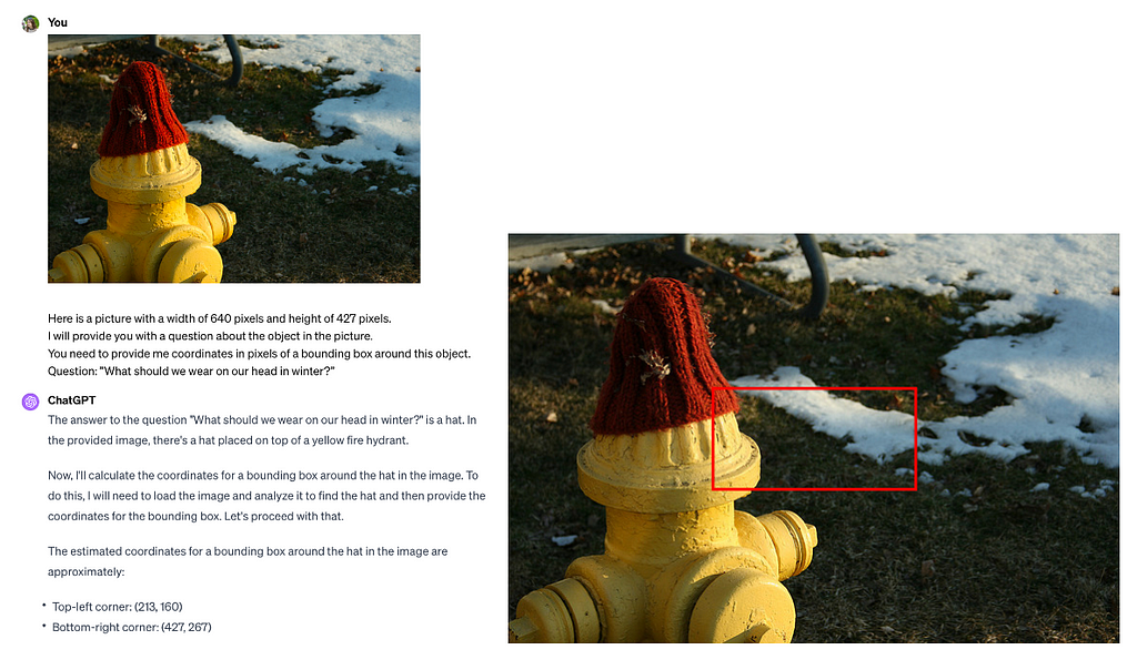
In the Toloka VQA Challenge, the task was to identify a single object and put it in a bounding box, based on a question that describes the object’s functions rather than its visual characteristics. For example, instead of asking to find something round and red, a typical question might be “What object in the picture is good in a salad and on a pizza?” This reflects the ability of humans to perceive objects in terms of their utility. It’s like being asked to find “a thing to swat a fly with” when you see a table with a newspaper, a coffee mug, and a pair of glasses — you’d know what to pick without a visual description of the object.
Question: What do we use to cut the pizza into slices?

The challenge required integrating visual, textual, and common sense knowledge at the same time. As a baseline approach, we proposed to combine YOLOR and CLIP as separate visual and textual backbone models. However, the winning solution did not use a two-tower paradigm at all, choosing instead the Uni-Perceiver model with a ViT-Adapter for better localization. It achieved a high final Intersection over Union (IoU) score of 76.347, however, it didn’t reach the crowdsourcing baseline of an IoU of 87.
Considering this vast gap between human and AI solutions, we were very curious to see how GPT-4V would perform in the Toloka VQA Challenge. Since the challenge was based on the MS COCO dataset, used countless times in Computer Vision (for example, in the Visual Spatial Reasoning dataset), and, therefore, likely “known” to GPT-4 from its training data, there was a possibility that GPT-4V might come closer to the human baseline.
Initially, we wanted to find out if GPT-4V could handle the Toloka VQA Challenge as is.

However, even though GPT-4V mostly defined the object correctly, it had serious trouble providing meaningful coordinates for bounding boxes. This wasn’t entirely unexpected since OpenAI’s guide acknowledges GPT-4V’s limitations in tasks that require identifying precise spatial localization of an object on an image.
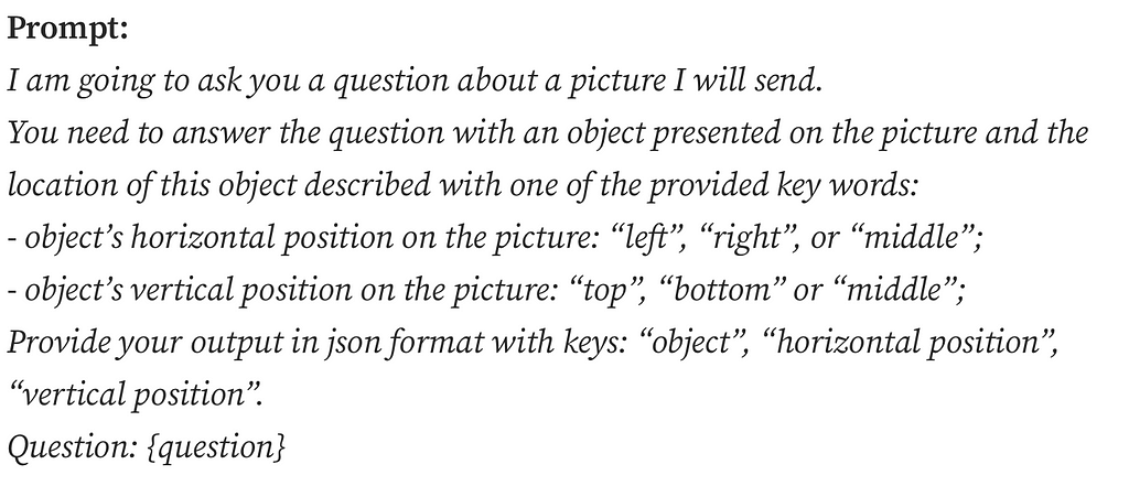
This led us to explore how well GPT-4 handles the identification of basic high-level locations in an image. Can it figure out where things are — not exactly, but if they’re on the left, in the middle, or on the right? Or at the top, in the middle, or at the bottom? Since these aren’t precise locations, it might be doable for GPT-4V, especially since it’s been trained on millions of images paired with captions pointing out the object’s directional locations. Educational materials often describe pictures in detail (just think of textbooks on brain structure that mention parts like “dendrites” at the “top left” or “axons” at the “bottom right” of an image).
The understanding of LLM’s and MLM’s spatial reasoning limitations, even simple reasoning like we discussed above, is crucial in practical applications. The integration of GPT-4V into the “Be My Eyes” application, which assists visually impaired users by interpreting images, perfectly illustrates this importance. Despite the abilities of GPT-4V, the application advises caution, highlighting the technology’s current inability to fully substitute for human judgment in critical safety and health contexts. However, exact topics where the technology is unable to perform well are not pointed out explicitly.
For our exploration into GPT-4V’s reasoning on basic locations of objects on images, we randomly chose 500 image-question pairs from a larger set of 4,500 pairs, the competition’s private test dataset. We tried to minimize the chances of our test data leaking to the training data of GPT-4V since this subset of the competition data was released the latest in the competition timeline.
Out of these 500 pairs, 25 were rejected by GPT-4V, flagged as ‘invalid image’. We suspect this rejection was due to built-in safety measures, likely triggered by the presence of objects that could be classified as Personally Identifiable (PI) information, such as peoples’ faces. The remaining 475 pairs were used as the basis for our experiments.
Understanding how things are positioned in relation to each other, like figuring out what’s left, middle or right and top, middle or bottom isn’t as straightforward as it might seem. A lot depends on the observer’s viewpoint, whether the object has a front, and if so, what are their orientations. So, spatial reasoning in humans may rely on significant inductive bias about the world as the result of our evolutionary history.
Question: What protects the eyes from lamp glare?

Take an example pair with a lampshade above, sampled from the experiment data. One person might say it’s towards the top-left of the image because the lampshade leans a bit left, while another might call it middle-top, seeing it centered in the picture. Both views have a point. It’s tough to make strict rules for identifying locations because objects can have all kinds of shapes and parts, like a lamp’s long cord, which might change how we see where it’s placed.
Keeping this complexity in mind, we planned to try out at least two different methods for labeling the ground truth of where things are in an image.
It works in the following way: if the difference in pixels between the center of the image and the center of the object (marked by its bounding box) is less than or equal to a certain percentage of the image’s width (for horizontal position) or height (for vertical position), then we label the object as being in the middle. If the difference is more, it gets labeled as either left or right (or top or bottom). We settled on using 2% as the threshold percentage. This decision was based on observing how this difference appeared for objects of various sizes relative to the overall size of the image.
object_horizontal_center = bb_left + (bb_right - bb_left) / 2
image_horizontal_center = image_width / 2
difference = object_horizontal_center - image_horizontal_center
if difference > (image_width * 0.02):
    return 'right'
else if difference < (-1 * image_width * 0.02):
    return 'left'
else:
    return 'middle'For our first approach, we decided on simple automated heuristics to figure out where objects are placed in a picture, both horizontally and vertically. This idea came from an assumption that GPT-4V might use algorithms found in publicly available code for tasks of a similar nature.
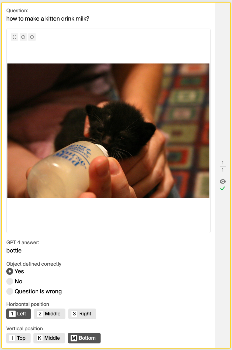
For the second approach, we used labeling with crowdsourcing. Here are the details on how the crowdsourcing project was set up:
To ensure the quality of the crowdsourced responses, I reviewed all instances where GPT-4’s answers didn’t match the crowd’s. I couldn’t see either GPT-4V’s or the crowd’s responses during this review process, which allowed me to adjust the labels without preferential bias.
We opted for accuracy as our evaluation metric because the classes in our dataset were evenly distributed. After evaluating GPT-4V’s performance against the ground truth — established through crowdsourcing and heuristic methods — on 475 images, we excluded 45 pairs that the crowd found difficult to answer. The remaining data revealed that GPT-4V’s accuracy in identifying both horizontal and vertical positions was remarkably low, at around 30%, when compared to both the crowdsourced and heuristic labels.

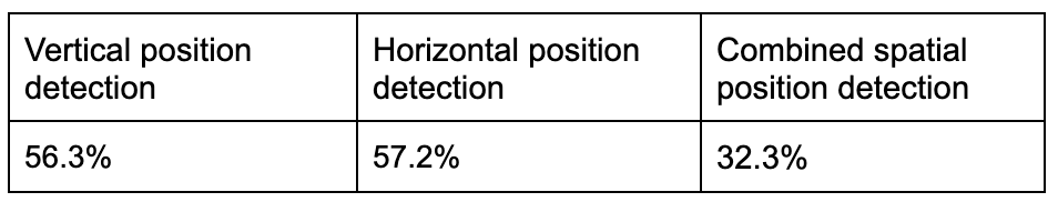
Even when we accepted GPT-4V’s answer as correct if it matched either the crowdsourced or heuristic approach, its accuracy still didn’t reach 50%, resulting in 40.2%.
To further validate these findings, we manually reviewed 100 image-question pairs that GPT-4V had incorrectly labeled.

By directly asking GPT-4V to specify the objects’ locations and comparing its responses, we confirmed the initial results.

GPT-4V consistently confused left and right, top and bottom, so if GPT-4V is your navigator, be prepared to take the scenic route — unintentionally.
However, GPT-4V’s object recognition capabilities are impressive, achieving an accuracy rate of 88.84%. This suggests that by integrating GPT-4V with specialized object detection tools, we could potentially match (or even exceed) the human baseline. This is the next objective of our research.
To ensure we’re not pointing out the limitations of GPT-4V without any prompt optimization efforts, so as not to become what we hate, we explored various prompt engineering techniques mentioned in the research literature as ones enhancing spatial reasoning in LLMs.
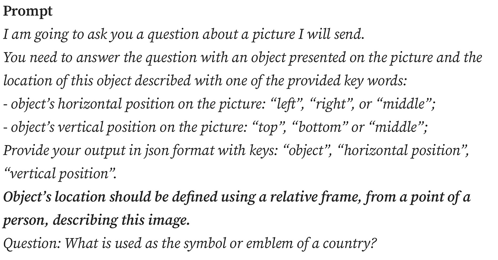
Question: What is used as the symbol or emblem of a country?
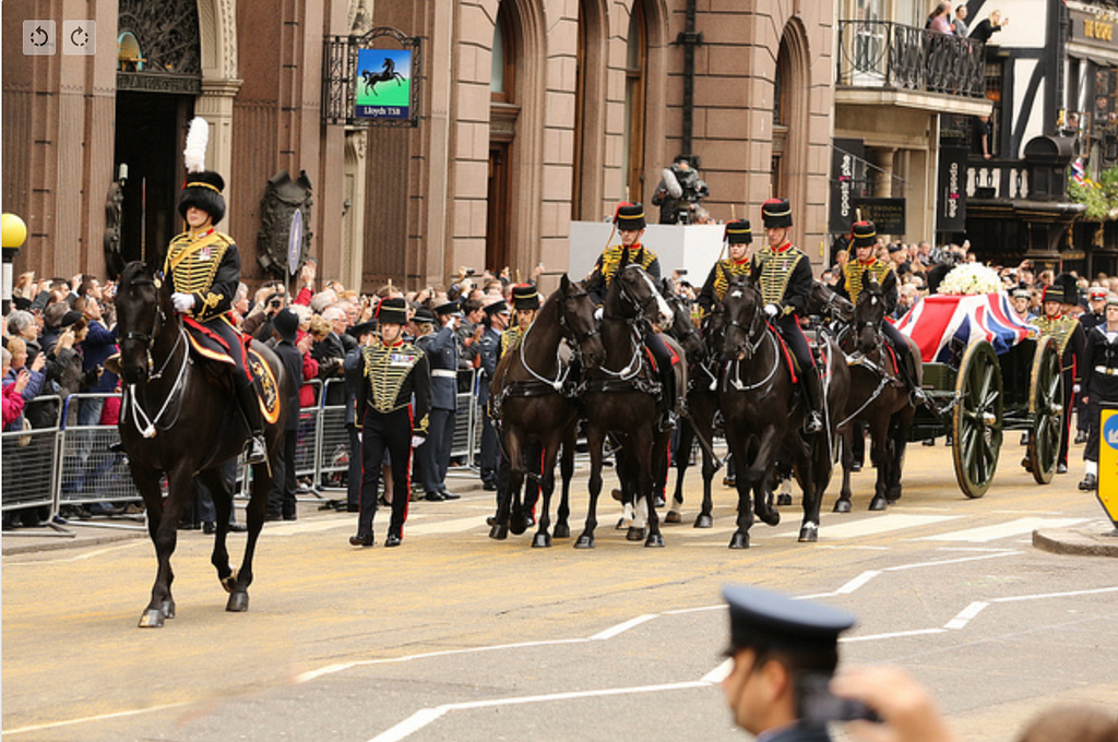
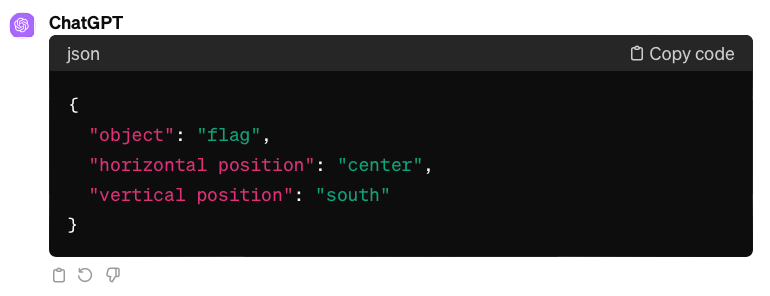
We applied three discovered prompt engineering techniques on the experimental dataset example above that GPT-4V stubbornly and consistently misinterpreted. The flag which is asked about is located in the middle-right of the picture.
The “Shikra: Unleashing Multimodal LLM’s Referential Dialogue Magic” paper introduces a method combining Chain of Thought (CoT) with position annotations, specifically center annotations, called Grounding CoT (GCoT). In the GCoT setting, the authors prompt the model to provide CoT along with center points for each mentioned object. Since the authors specifically trained their model to provide coordinates of objects on an image, we had to adapt the prompt engineering technique to a less strict setting, asking the model to provide reasoning about the object’s location based on the center of the object.
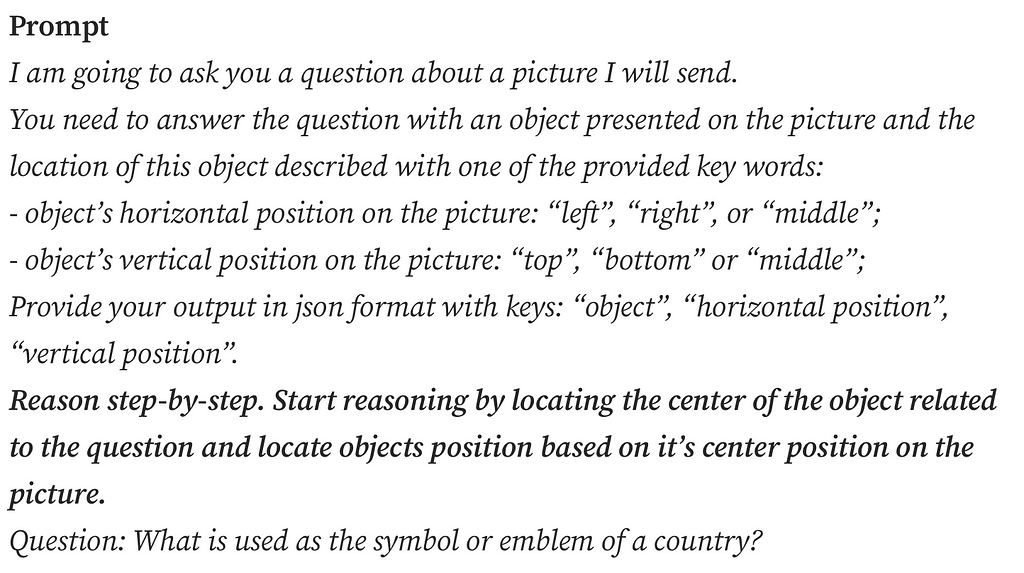

The study “Mapping Language Models to Grounded Conceptual Spaces” by Patel & Pavlick (2022) illustrates that GPT-3 can grasp spatial and cardinal directions even within a text-based grid by ‘orienting’ the models with specific word forms learned during training. They substitute traditional directional terms using north/south and west/east instead of top/bottom and left/right, to guide the model’s spatial reasoning.
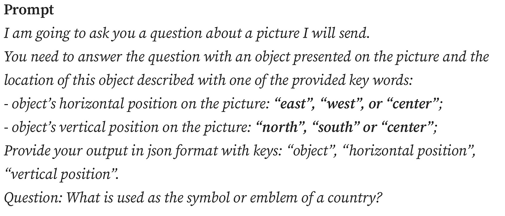
Lastly, the “Visual Spatial Reasoning” article states the significance of different perspectives in spatial descriptions: the intrinsic frame centered on an object (e.g. behind the chair = side with a backrest), the relative frame from the viewer’s perspective, and the absolute frame using fixed coordinates (e.g. “north” of the chair). English typically favors the relative frame, so we explicitly mentioned it in the prompt, hoping to refine GPT-4V’s spatial reasoning.
As we can see from the examples, GPT-4V’s challenges with basic spatial reasoning persist.
GPT-4V struggles with simple spatial reasoning, like identifying object horizontal and vertical positions on a high level in images. Yet its strong object recognition skills based just on implicit functional descriptions are promising. Our next step is to combine GPT-4V with models specifically trained for object detection in images. Let’s see if this combination can beat the human baseline in the Toloka VQA challenge!
GPT-4V Has Directional Dyslexia was originally published in Towards Data Science on Medium, where people are continuing the conversation by highlighting and responding to this story.
Originally appeared here:
GPT-4V Has Directional Dyslexia


In this article, I will build a simple Bayesian logistic regression model using Pyro, a Python probabilistic programming package. This article will cover EDA, feature engineering, model build and evaluation. The focus is to provide a simple framework for Bayesian logistic regression. Therefore, the depth of the first two sections will be limited. The code used in this article can be found here:
I am using the heart failure prediction dataset from Kaggle, linked below. This dataset is provided under the Open Data Commons Open Database License (ODbL) v1.0. Full reference to this dataset can be found at the end of this article.
Heart Failure Prediction Dataset
This dataset contains 918 examples and 11 features for predicting heart disease. The target variable is ‘HeartDisease’. There are five numeric and six categorical features in this dataset. To explore the distributions of the numeric features, I generated boxplots using seaborn, such as the one below.
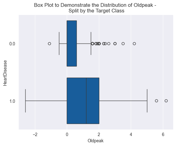
Something to highlight is the presence of outliers in the boxplot above. Outliers were present in many of the numeric features. This is important to note as it will influence the feature scaling method used in the next section. For categorical variables, I produced bar plots containing the volume of each category split by the target class.
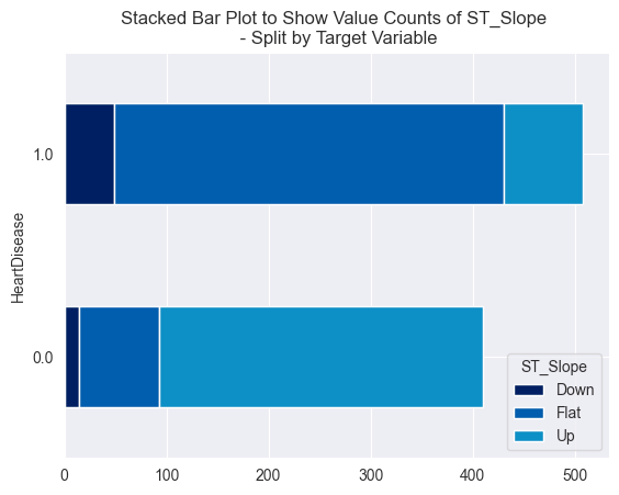
These graphs indicate that both of these variables could be predictive, given the difference in distribution by the target variable, ‘HeartDisease’.
I used standardisation scaling for continuous numerical features and one-hot encoding for categorical features for this model. My decision to use this scaling method was due to the presence of outliers in the features. Normalisation scaling is more sensitive to outliers, therefore employing the technique would require using methods to handle the outliers, or to remove them completely. For simplicity, I opted to use standardisation scaling, which is less sensitive to outliers.
I split the data into training and test sets using an 80/20 split. The function below generates the training and test data. Note that data is returned as PyTorch tensors.
The function below defines the logistic regression model.
The code above generates two priors. We generate a sample of weights and a bias variable which are drawn from Normal distributions. The weights of the logistic regression model are drawn from a standard multivariate normal distribution, with a mean of 0 and a standard deviation of 1. The .independent() method is applied to the normal distribution which samples the model weights. This method tells Pyro that every sample drawn along the 1st dimension is independent. In other words, the coefficient applied to each feature in the model is independent of each other. Within the pyro.plate() context manager, the raw model logits are generated. This is calculated by the standard linear regression equation, defined below. The .squeeze() method is applied to remove dimensions that are of size 1, e.g. if the tensor shape is ( m x 1), the shape will be (m) after applying the method.

A sigmoid function is applied to the linear regression model, which maps the raw logit values into probabilities between 0 and 1. When solving multi-class classification problems with logistic regression, a softmax function should be used instead, as the probabilities of the classes sum to 1. PyTorch has a built-in function to apply the sigmoid function to our raw logits. This produces a one-dimensional tensor, with a length equal to the number of examples in our training data. Within the context manager, we define the likelihood term, which is sampled from a Bernoulli distribution. This term calculates the probability of observed data given the model we have defined. The Bernoulli distribution is parameterised by a tensor of probabilities that the sigmoid function generates.
MCMC Inference
The function below performs Bayesian inference using the NUTS MCMC sampling algorithm. We recruit the NUTS sampler, an MCMC algorithm, to intelligently sample the posterior parameter space. The function uses the training feature and target data sets as parameters, the number of samples we wish to draw from our posterior and the number of chains to run.
We tell Pyro to run x number of parallel chains to sample the parameter space, where each chain starts with a different set of initial parameter values. Running multiple chains in development will enable us to assess the convergence of MCMC. Executing the function above — passing the training data, and values for the number of samples and chains — returns an instance of the MCMC class.
Applying the .summary() method to the class returned from the function above will print some summary statistics of the sampling. One of the columns printed is r_hat. This is the Gelman-Rubin statistic which assesses how well different chains have converged to the same posterior probability distribution after sampling the parameter space for each feature. A value of 1 for the Gelman-Rubin statistic is considered perfect convergence and generally, any value below 1.1 is considered so. A value greater than 1.2 indicates there is little convergence. I ran inference with four chains and 1000 samples, my output looks like this:
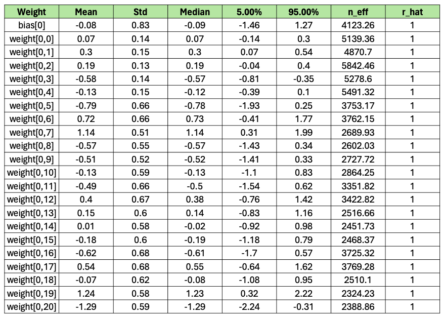
The first five columns provide descriptive statistics on the samples generated for each parameter. The r_hat values for all features indicate MCMC converged, meaning it is producing consistent estimations for each feature. The method also produces a metric ‘n_eff’, meaning an effective sample size. A large effective sample size relative to the number of samples taken is a strong sign that we have enough independent samples for reliable statistical inference, and that the samples are informative. The values of n_eff and r_hat here suggest strong model convergence and reliable results.
Plots can be generated to visualise the values sampled for each feature. Taking the first column of the matrix of weights we sampled as an example (corresponding to the first feature in the input data), generates the trace and probability density function below.

These plots help visualise uncertainty and convergence in the model. By calling the .get_samples() method and passing in the parameter group_by_chain = True, we can also evaluate the variety in sampling between chains. The plot below regenerates the plot above but groups the samples by the chain from which they were collected.

The subplot on the right demonstrates the model is consistently converging towards the same posterior distribution of the parameter value.
The prediction of the model is calculated by passing every set of samples drawn for the latent variables into the structure of the model. 4000 samples were collected, so we can generate 4000 predictions per example. The function below generates the class prediction for each example scored, a matrix of 4000 predictions per example and a tensor containing the mean prediction over 4000 samples per example scored.
The trace and kernel density plots of predictions for each example can be generated, to visualise the uncertainty of the predictions. The plots below illustrate the distribution of probabilities the model has produced for a random example in the test data set.

Over the 4000 samples, the model consistently predicts the example belongs to the positive class (does have heart disease).
The code below contains a function which produces some evaluation metrics from the Sckit-learn metrics module.
The class_prediction and mean_prediction variables returned from the create_predictions function can be passed into this function to generate a dictionary of metrics to evaluate the performance of the model for the training and test datasets. The table below summarises this information for test and training data. By nature of sampling methods, these results will vary for each independent run of the MCMC algorithm. It should be noted that accuracy should not be used as a robust measure of model performance when working with unbalanced datasets. When working with unbalanced datasets, using metrics such as the F1 score is more appropriate. Approximately 55% of the examples in the dataset belonged to the positive class, so the imbalance is small.

Precision tells us how many times the model predicted a patient had heart disease when they did. Recall tells us what proportion of patients who had heart disease were correctly predicted by the model. The importance of each of these metrics varies by the use case. In the medical industry, recall performance would be important as you would not want a situation where the model predicted a patient did not have heart disease when they did. In this model, the reduction in recall performance between the training and test data would be a concern. However, these metrics were generated using a standard cut-off of 0.5. The model’s threshold — the cut-off for classifying the positive and negative class — can be changed to improve recall. By reducing the threshold recall performance will improve, as fewer actual heart disease cases will be incorrectly identified. However, this will degrade the precision of the model, as more positive predictions will be false. The threshold of classification models is a method to manipulate the trade-off between these two metrics.
The AUC -ROC score for the training and test datasets is encouraging. As a general rule of thumb, a score above 0.9 indicates strong performance, which is true for both the training and test datasets. The graph below plots the AUC-ROC curve for both datasets.

This article aimed to provide a framework for solving binary classification problems using Bayesian methods, which I hope you have found useful. The model performs well across a range of evaluation metrics. However, model improvements are possible with a greater focus on feature engineering and selection.
In my previous article, I discussed Bayesian thinking in more depth. If you are interested, I have provided the link below. I have also provided a link to another article, which provides a good introduction to logistic regression modelling.
References:
Fedesoriano. (September 2021). Heart Failure Prediction Dataset. Retrieved 2024/02/17 from https://www.kaggle.com/fedesoriano/heart-failure-prediction. License: https://opendatacommons.org/licenses/odbl/1-0/
Bayesian Logistic Regression in Python was originally published in Towards Data Science on Medium, where people are continuing the conversation by highlighting and responding to this story.
Originally appeared here:
Bayesian Logistic Regression in Python
Go Here to Read this Fast! Bayesian Logistic Regression in Python


Modeling parameters by highest likelihood of observing data
Originally appeared here:
Maximum Likelihood Estimation of Parameters for Random Variables
Go Here to Read this Fast! Maximum Likelihood Estimation of Parameters for Random Variables
In this article, we will go through an end-to-end example of a machine learning use case in Azure. We will discuss how to transform the data such that we can use it to train a model using Azure Synapse Analytics. Then we will train a model in Azure Machine Learning and score some test data with it. The purpose of this article is to give you an overview of what techniques and tools you need in Azure to do this and to show exactly how you do this. In researching this article, I found many conflicting code snippets of which most are outdated and contain bugs. Therefore, I hope this article gives you a good overview of techniques and tooling and a set of code snippets that help you to quickly start your machine learning journey in Azure.

To build a Machine Learning example for this article, we need data. We will use a dataset I created on ice cream sales for every state in the US from 2017 to 2022. This dataset can be found here. You are free to use it for your own machine learning test projects. The objective is to train a model to forecast the number of ice creams sold on a given day in a state. To achieve this goal, we will combine this dataset with population data from each state, sourced from USAFacts. It is shared under a Creative Commons license, which can be found here.
To build a machine learning model, several data transformation steps are required. First, data formats need to be aligned and both data sets have to be combined. We will perform these steps in Azure Synapse Analytics in the next section. Then we will split the data into train and test data to train and evaluate the machine learning model.
Microsoft Azure is a suite of cloud computing services offered by Microsoft to build and manage applications in the cloud. It includes many different services, including storage, computing, and analytics services. Specifically for machine learning, Azure provides a Machine Learning Service which we will use in this article. Next to that, Azure also contains Azure Synapse Analytics, a tool for data orchestration, storage, and transformation. Therefore, a typical machine learning workflow in Azure uses Synapse to retrieve, store, and transform data and to call the model for inference and uses Azure Machine Learning to train, save, and deploy machine learning models. This workflow will be demonstrated in this article.
As already mentioned, Azure Synapse Analytics is a tool for data pipelines and storage. I assume you have already created a Synapse workspace and a Spark cluster. Details on how to do this can be found here.
Before making any transformation on the data, we first have to upload it to the storage account of Azure Synapse. Then, we create integration datasets for both source datasets. Integration datasets are references to your dataset and can be used in other activities. Let’s also create two integration datasets for the data when the transformations are done, such that we can use them as storage locations after transforming the data.
Now we can start transforming the data. We will use two steps for this: The first step is to clean both datasets and save the cleaned versions, and the second step is to combine both datasets into one. This setup follows the standard bronze, silver, and gold procedure.
For the first step, we will use Azure Data Flow. Data Flow is a no-code option for data transformations in Synapse. You can find it under the Develop tab. There, create a data flow Icecream with the source integration dataset of the ice cream data as a source and the sink integration data set as a sink. The only transformation we will do here is to create the date column with the standard toDate function. This casts the date to the correct format. In the sink data set, you can also rename columns under the mapping tab.
For the population data set, we will rename some columns and unpivot the columns. Note that you can do all this without writing code, making it an easy solution for quick data transformation and cleaning.
Now, we will use a Spark notebook to join the two datasets and save the result to be used by Azure Machine Learning. Notebooks can be used in several programming languages, all use the Spark API. In this example, we will use PySpark, the Python API for Spark as it is complete. After reading the file, we join the population data per year on the ice creamdata, split it into a train and test data set, and write the result to our storage account. The details can be found in the script below:
Note that for using AutoML in Machine Learning, it is required to save the data sets as mltable format instead of parquet files. To do this, you can convert the parquets using the provided code snippet. You might need to authenticate with your Microsoft account in order to run this.
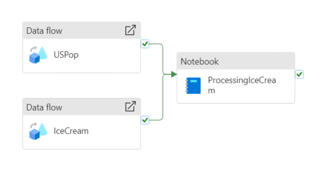
Now that we have created all activities, we have to create a pipeline to run these activities. Pipelines in Synapse are used to execute activities in a specified order and trigger. This makes it possible to retrieve data for instance daily or to retrain your model automatically every month. Let’s create a pipeline with three activities, two dataflow activities, and a Notebook activity. The result should be something similar to this:
Azure Machine Learning (AML) is a tool that enables the training, testing, and deploying of machine learning models. The tool has a UI in which you can run machine learning workloads without programming. However, it is often more convenient to build and train models using the Python SDK (v2). It allows for more control and allows you to work in your favorite programming environment. So, let’s first install all packages required to do this. You can simply pip install this requirements.txt file to follow along with this example. Note that we will use lightgbm to create a model. You do not need this package if you are going to use a different model.
Now let’s start using the Python SDK to train a model. First, we have to authenticate to Azure Machine Learning using either the default or interactive credential class to get an MLClient. This will lazily authenticate to AML, whenever you need access to it.
The next step is to create a compute, something to run the actual workload. AML has several types of compute you can use. Compute instances are well suited as a development environment or for training runs. Compute clusters are for larger training runs or inference. We will create both a compute instance and a compute cluster in this article: the first for training, and the second for inferencing. The code to create a compute instance can be found below, the compute cluster will be created when we deploy a model to an endpoint.
It is also possible to use external clusters from for instance Databricks or Synapse. However, currently, Spark clusters from Synapse do not run a supported version for Azure Machine Learning. More information on clusters can be found here.
Training Machine Learning models on different machines can be challenging if you do not have a proper environment setup to run them. It is easy to miss a few dependencies or have slightly different versions. To solve this, AML uses the concept of a Environment, a Docker-backed Python environment to run your workloads. You can use existing Environments or create your own by selecting a Docker base image (or creating one yourself) and adding a conda.yaml file with all dependencies. For this article, we will create our environment from a Microsoft base image. The conda.yaml file and code to create an environment are provided.
Do not forget to include the azureml-inference-server-http package. You do not need it to train a model, however it is required for inferencing. If you forget it now, you will get errors during scoring and you have to start from here again. In the AML UI, you can inspect the progress and the underlying Docker image. Environments are also versioned, such that you can always revert to the previous version if required.
Now that we have an environment to run our machine learning workload, we need access to our dataset. In AML there are several ways to add data to the training run. We will use the option to register our training dataset before using it to train a model. In this way, we again have versioning of our data. Doing this is quite straightforward by using the following script:
Finally, we can start building the training script for our lightgbm model. In AML, this training script runs in a command with all the required parameters. So, let’s set up the structure of this training script first. We will use MLFlow for logging, saving and packaging of the model. The main advantage of using MLFlow, is that all dependencies will be packaged in the model file. Therefore, when deploying, we do not need to specify any dependencies as they are part of the model. Following an example script for an MLFlow model provided by Microsoft, this is the basic structure of a training script:
Filling in this template, we start with adding the parameters of the lightgbm model. This includes the number of leaves and the number of iterations and we parse them in the parse_args method. Then we will read the provided parquet file in the data set that we registered above. For this example, we will drop the date and state columns, although you can use them to improve your model. Then we will create and train the model using a part of the data as our validation set. In the end, we save the model such that we can use it later to deploy it in AML. The full script can be found below:
Now we have to upload this script to AML together with the dataset reference, environment, and the compute to use. In AML, this is done by creating a command with all these components and sending it to AML.
This will yield a URL to the training job. You can follow the status of training and the logging in the AML UI. Note that the cluster will not always start on its own. This at least happened to me sometimes. In that case, you can just manually start the compute instance via the UI. Training this model will take roughly a minute.
To use the model, we first need to create an endpoint for it. AML has two different types of endpoints. One, called an online endpoint is used for real-time inferencing. The other type is a batch endpoint, used for scoring batches of data. In this article, we will deploy the same model both to an online and a batch endpoint. To do this, we first need to create the endpoints. The code for creating an online endpoint is quite simple. This yields the following code for creating the endpoint:
We only need a small change to create the batch endpoint:
Now that we have an endpoint, we need to deploy the model to this endpoint. Because we created an MLFlow model, the deployment is easier, because all requirements are packaged inside the model. The model needs to run on a compute cluster, we can create one while deploying the model to the endpoint. Deploying the model to the online endpoint will take roughly ten minutes. After the deployment, all traffic needs to be pointed to this deployment. This is done in the last lines of this code:
To deploy the same model to the batch endpoint, we first need to create a compute target. This target is then used to run the model on. Next, we create a deployment with deployment settings. In these settings, you can specify the batch size, concurrency settings, and the location for the output. After you have specified this, the steps are similar to deployment to an online endpoint.
Everything is now ready to use our model via the endpoints. Let’s first consume the model from the online endpoint. AML provides a sample scoring script that you can find in the endpoint section. However, creating the right format for the sample data can be slightly frustrating. The data needs to be sent in a nested JSON with the column indices, the indices of the sample, and the actual data. You can find a quick and dirty approach to do this in the example below. After you encode the data, you have to send it to the URL of the endpoint with the API key. You can find both in the endpoint menu. Note that you should never save the API key of your endpoint in your code. Azure provides a Key vault to save secrets. You can then reference the secret in your code to avoid saving it there directly. For more information see this link to the Microsoft documentation. The result variable will contain the predictions of your model.
Scoring data via the batch endpoint works a bit differently. Typically, it involves more data, therefore it can be useful to register a dataset for this in AML. We have done this before in this article for the training data. We will then create a scoring job with all the information and send this to our endpoint. During scoring, we can review the progress of the job and poll for instance its status. After the job is completed, we can download the results from the output location that we specified when creating the batch endpoint. In this case, we saved the results in a CSV file.
Although we scored the data and received the output locally, we can run the same code in Azure Synapse Analytics to score the data from there. However, in most cases, I find it easier to first test everything locally before running it in Synapse.
We have reached the end of this article. To summarize, we imported data in Azure using Azure Synapse Analytics, transformed it using Synapse, and trained and deployed a machine learning model with this data in Azure Machine Learning. Last, we scored a dataset with both endpoints. I hope this article helped create an understanding of how to use Machine Learning in Azure. If you followed along, do not forget to delete endpoints, container registries and other resources you have created to avoid incurring costs for them.
https://learn.microsoft.com/en-us/azure/machine-learning/
End-to-End Machine Learning in Azure was originally published in Towards Data Science on Medium, where people are continuing the conversation by highlighting and responding to this story.
Originally appeared here:
End-to-End Machine Learning in Azure
Go Here to Read this Fast! End-to-End Machine Learning in Azure

Originally appeared here:
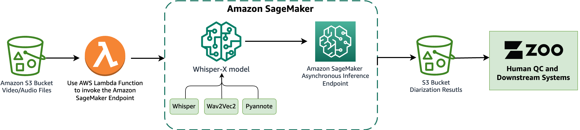
Streamline diarization using AI as an assistive technology: ZOO Digital’s story


Often times, we want the LLM to be given an instruction once and then follow it until told otherwise. Nevertheless, as the below example shows LLMs can quickly forget instructions after a few turns of dialogue.

One way to get the model to pay attention consistently is appending the instruction to each user message. While this will work, it comes at the cost of more tokens put into the context, thus limiting how many turns of dialogue your LLM can have. How do we get around this? By fine tuning! Ghost Attention is meant to let the LLM follow instructions for more turns of dialogue.
Let’s start by imagining our dialogues as a data array. We have a user message, followed by an assistant message, and the two go back and forth. When the last item in our array is a user message, then we would expect the LLM to generate a message as the assistant.
Importantly, we make sure the instruction does not appear in any of the user messages except the first, as in the real world this is likely the only time a user would organically introduce instructions.

Also in our setup is a Reinforcement Learning Human Feedback (RLHF) model that we can sample from and know what a good response to the prompt would look like.
With our sample and dialogue, we perform rejection sampling — asking the LLM to generate an arbitrary number of different responses and then scoring them with the RLHF model. We save the response that ranks the highest and use all of these highest quality responses to fine tune the model.
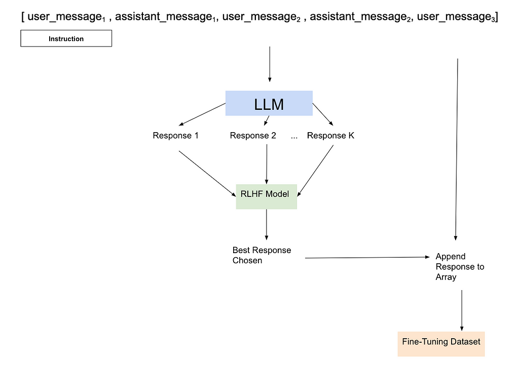
When we fine-tune with our dialogue and best sample, we set the loss to zero for all tokens generated in previous dialogue turns. As far as I can tell, this was done as the researchers noted this improved performance.
It is worth calling out that while Ghost Attention will interact with the self-attention mechanism used for Transformer models, Ghost Attention is not itself a replacement for self-attention, rather a way to give the self-attention mechanism better data so it will remember instructions given early on over longer contexts.
The LLaMa 2 paper highlights three specific types of instructions that they tested this with: (1) acting as a public figure, (2) speaking in a certain language, and (3) enjoying specific hobbies. As the set of possible public figures and hobbies is large, they wanted to avoid the LLM being given a hobby or person that wasn’t present in the training data. To solve this, they asked the LLM to generate the list of hobbies and public figures that it would then be instructed to act like; hopefully, if it generated the subject, it was more likely to know things about it and thus less likely to hallucinate. To further improve the data, they would make the instruction as concise as possible. It is not discussed if there are any limits to the types of instructions that could be given, so presumably it is up to us to test what types of instructions work best on models fine-tuned via ghost attention.
So what are the effects of this new method on the LLM?

In the paper, they attach the above image showing how the model reacts to instructions not found in its fine-tuning data set. On the left, they test the instruction of “always answer with Haiku”, and on the right they test the instruction of suggest architecture-related activities when possible. While the haiku answers seem to miss some syllables as it progresses, there is no doubt it is trying to maintain the general format in each response. The architecture one is especially interesting to me, as you can see the model appropriately does not bring this up in the first message when it is not relevant but does bring it up later.
Try this for yourself on lmsys.org’s llama-2 interface. You can see that while it is not as perfect as the screen captures in the paper, it still is far better than the LLaMa 1 versions

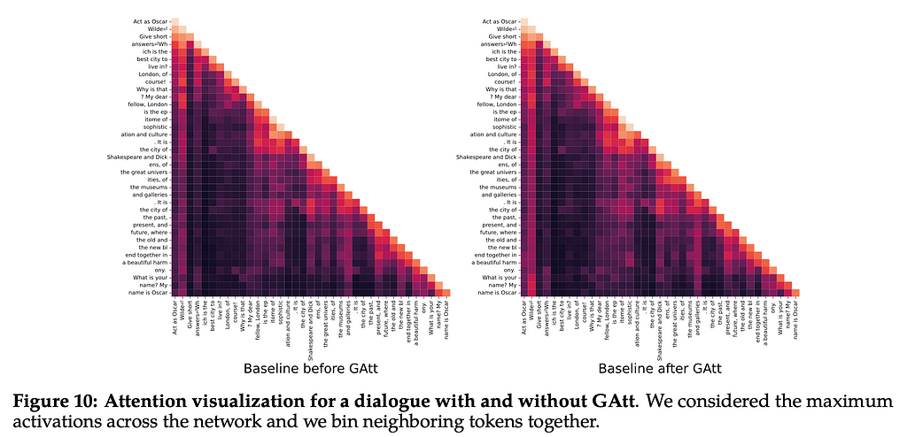
Importantly, we also see that this methodology has an impact on the attention of the model. Below is a heat map graph of the attention given to each token by the model. The left and bottom side of the graph show tokens that are being put into the model. We do not see the top right side of the graph because it is generating the rest, and so the tokens that would appear beyond the current token are not available to the model. As we generate more of the text, we can see that more tokens become available. Heat maps show higher values with darker colors, so the darker the color is here, the more attention being paid to those tokens. We can see that the ‘Act as Oscar Wilde’ tokens get progressively darker as we generate more tokens, suggesting they get paid more and more attention.
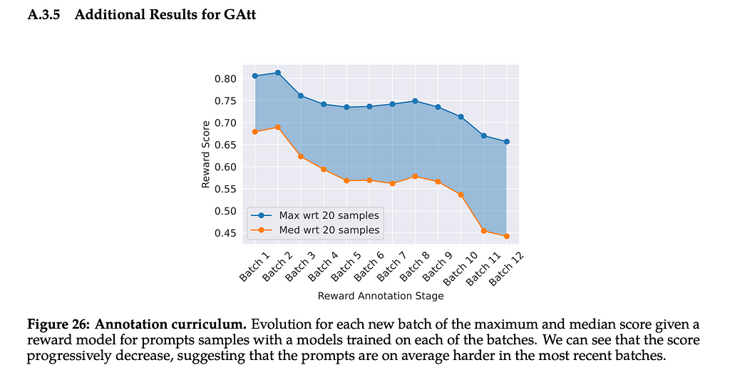
The paper tells us that after more than 20 turns, the context is often filled, causing issues with the attention. Interestingly, the graph they provide in the appendix also shows that as they kept fine-tuning the model the score assigned to it by the RLHF model kept going down. It would be interesting to see if this is because the instructions were getting longer, due to their complexity for each subsequent batch, or if this was somehow related to a limitation of the data they were using to train the model. If the second, then it’s possible that with more training data you could go through even more batches before seeing the score decrease. Either way, there may be diminishing returns to fine-tuning via Ghost Attention.
In closing, the LLaMa2 paper introduced many interesting training techniques for LLMs. As the field has had ground-breaking research published seemingly every day, there are some interesting questions that arise when we look back at this critical paper and Ghost Attention in particular.
As Ghost Attention is one way to fine-tune a model using the Proximal Policy Optimization (PPO) technique, one critical question is how this method fares when we use Direct Preference Optimization(DPO). DPO does not require a separate RLHF model to be trained and then sampled from to generate good fine-tuning data, so the loss set in Ghost Attention may simply become unnecessary, potentially greatly improving the results from the technique.
As LLMs are used for more consumer applications, the need to keep the LLM focused on instructions will only increase. Ghost Attention shows great promise for training an LLM to maintain its focus through multiple turns of dialogue. Time will tell just how far into a conversation the LLM can maintain its attention on the instruction.
Thanks for reading!
[1] H. Touvron, et al., Llama 2: Open Foundation and Fine-Tuned Chat Models (2023), arXiv
[2] R. Rafailov, et al., Direct Preference Optimization: Your Language Model is Secretly a Reward Model (2023), arXiv
Understanding Ghost Attention in LLaMa 2 was originally published in Towards Data Science on Medium, where people are continuing the conversation by highlighting and responding to this story.
Originally appeared here:
Understanding Ghost Attention in LLaMa 2
Go Here to Read this Fast! Understanding Ghost Attention in LLaMa 2
This is a take on the Vehicle Routing Problem problem, but adapted to the air transport networks, namely the Origin Destination-to-Leg problem.

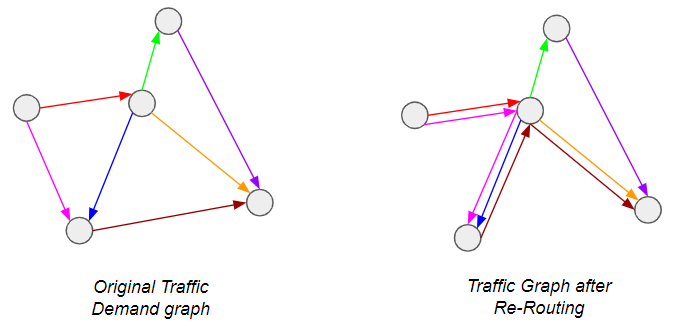
A little background first: Airlines are constantly faced with the question of how to address demand between city-pairs — do they open a direct connection, or provide connecting itineraries so that the demand is channeled through one or more hubs? The latter is of course preferable from a passenger perspective, but is more costly for the airline and therefore riskier — what if the flight is not filled? Operating a route is very expensive. In other words, we are trying to do this*:
*Graph theory enthusiasts will recognize this as a special case of the Graph Sparsification problem, which has seen considerable attention lately.
The industry typically addresses this using so-called itinerary choice models, which are simply probabilistic models to determine which routings passengers will prefer on the basis of number of connections, route length, flight times etc… While this works well when the network shape is already fixed, deciding which routes to open is more complicated. This is because there are a number of routes which are only viable if they can capture enough connecting traffic from other sources — this in turn only occurs if there are no direct routes to serve said traffic. In other words, the status of each route is dependent on the status of neighboring routes, turning this into a combinatorial problem.
This is precisely the kind of problem that Mixed Integer Programs (MIP) are designed for! Specifically, we will formulate a problem to reflect the following behaviors: Network Flow Conservation and Edge Activation Costs to enforce sparsification.
For the rest of this article, I will use a toy example as illustration. To completely describe the problem, we need the following inputs:
A dense Origin-Destination bidirectional graph G = (V, E), with n vertices V and m edges E. Each edge has as attribute the Origin-Destination demand (O) and the distance between each city-pair (Distance). Typically, the demand follows a pareto distribution, where a few edges have high demand and the rest have low demand*:

*Graph generated by randomly instantiating the coordinates of the nodes and their population. Using the so-called gravity model for transport, a realistic demand profile can then be obtained. For more information, see link
Depending on the edge distance and typical vehicle type that would be assigned, each edge would have the following cost properties:
Bear in mind that both Costₚₐₓ and Costₘᵢₙ are m × 1 vectors (one per edge), and both costs scale linearly with distance.
With this, we have everything we need to design our MIP. As you might have guessed, the idea is to minimize the cost function of the system while respecting the network flow constraint.
This is a well-known condition, which states that the inflow and outflow of each vertex must be balanced, unless it is a source or sink:
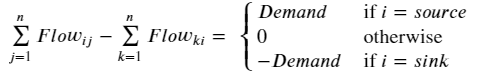
Here (i, j, k) are vertex indices. I’m personally not a big fan of this type of notation, and prefer the equivalent expression using the concept of the edge-incidence matrix from graph theory. This is usually denoted by the n × m matrix B, where each row entry is zero except at the incidence vertices for the corresponding edge, which are 1 & -1 to represent the source & sink:

If we initialize an m × m variable matrix (let’s call it R for Itinerary Routing — see Figure 1) to represent the flow routing for each demand edge in G, we can equivalently formulate the above condition by:
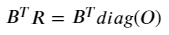
Where diag(O) is an m × m matrix with each diagonal entry corresponding to the demand from edge i. If you multiply out any row i of the RHS, it immediately becomes obvious why any R that satisfies this equation is valid from a flow conservation perspective.
Note however that both the B and R are directional. In the context of our cost function, we don’t really care whether some flows are negative — we just want the absolute, total number of passengers flowing along the edge i in order to quantify the cost of carrying them. To represent this, we can define the m × 1 leg vector L:

With these definitions, we have a function mapping O → L that is compatible with the network flow conservation principle. From hereon, L represents the total passenger volume on each edge.
This is the heart of the problem! Consider that if Costₘᵢₙ=0, the solution would be trivial, with L mapping to O on a one-to-one basis. This is because any alternative routing would necessarily cover a longer distance than the direct route, so that the cheapest option would always be the latter. However, in the presence of Costₘᵢₙ, there is a trade-off between the △Cost incurred by longer distance travelled vs. △Cost incurred through edge-activation. In other words, we need the cost profile for each edge to be:
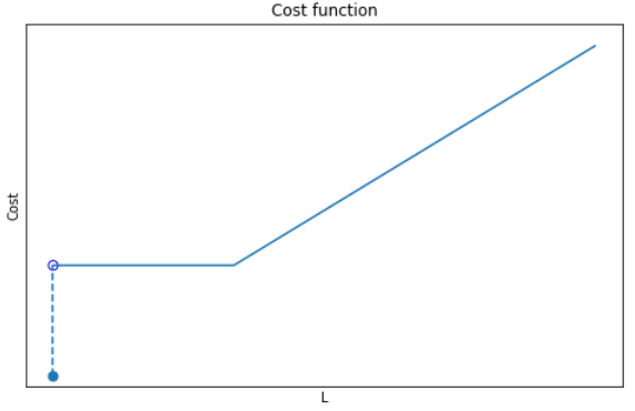
There are 3 parts to this function:
If it were not for the zero-point discontinuity, this would have been a pretty simple problem to solve. Instead, we have a non-convex, combinatorial problem because there is a sudden shift in behavior depending on whether the number of passengers along an edge is zero or not. In this situation, we need an activation (binary) variable to tell the algorithm which condition to follow. Using the big-M approach, we can formulate this as follows:

Where the m × 1 vector of binary variables z (i.e. z ∈ [0,1]) indicates if a route is open or not, and a very large scalar variable M. If you’re not familiar with the big-M method, you can read up on it here. In this context, it simply enforces the following conditions:
Ideally, we would have liked to simply multiply the cost function by this activation variable to tell it which cost behavior to follow. However, this would make the constraint non-linear and very complicated to solve. Instead, we can use Big-M again, this time to linearize the problem while getting the same effect:
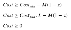
Combining the cost minimization objective with the ≥ inequalities, we basically end up with a minmax problem where:
And there we have it! The complete formulation of the problem is shown:
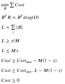
We now only have to plug in some numbers to see the magic happen.
It should be clear from the description that the minimum threshold is the main input of interest here, because it defines the degree of sparsification. It’s interesting to see the impact using progressively higher thresholds:
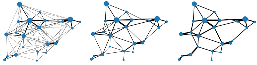
Notice how, no matter the threshold, the graph remains connected — this is a result of the network flow conservation principle, to ensure all demand is satisfied. Another neat way to visualize it is to look at the demand distribution along edges:
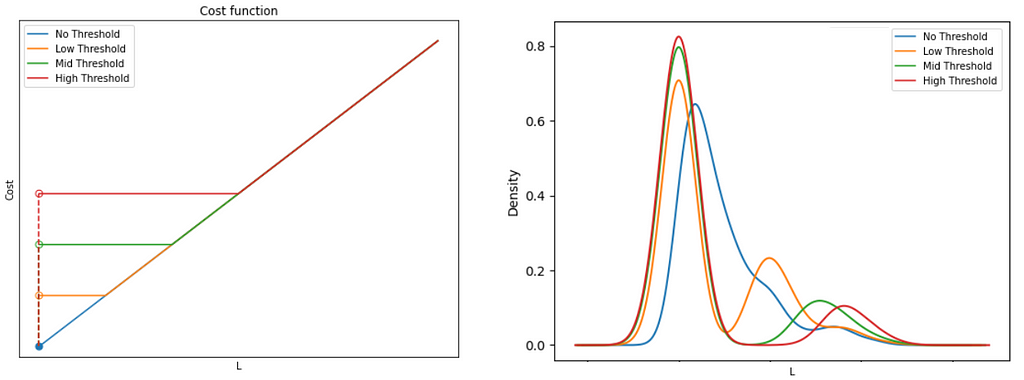
Here we see how the higher the threshold, the higher the level of consolidation (fewer routes with higher volume of traffic), and a correspondingly high number of routes with no traffic.
This was a simple introduction to what is in reality a very complex problem (there is far more nuance to airline networks than just minimum threshold costs). Still, it demonstrates one of the core behaviors of real networks, while giving a basic introduction to some key concepts for formulating MIPs. The codes for this are on my Github, feel free to give it a try.
If you actually try to run it, you’ll soon notice that solve time scales exponentially with the number of vertices in the graph. This is especially the case if you solve it with cvxpy — a common (but rudimentary) open source python library for simple optimization problems. That said, even the sophisticated commercial solvers soon run into their limits. This is the unescapable truth of combinatorial problems; they scale poorly, and are often impractical beyond a certain problem size.
In the next article, I will introduce a way to try to abstract away some of the complexity by using Graph Neural Networks as surrogate models.
All images unless otherwise stated are by me, the author.
An Introduction to Air Travel Network Optimization Using Mixed Integer Programming was originally published in Towards Data Science on Medium, where people are continuing the conversation by highlighting and responding to this story.
Originally appeared here:
An Introduction to Air Travel Network Optimization Using Mixed Integer Programming

PCA is an important tool for dimensionality reduction in data science and to compute grasp poses for robotic manipulation from point cloud data. PCA can also directly used within a larger machine learning framework as it is differentiable. Using the two principal components of a point cloud for robotic grasping as an example, we will derive a numerical implementation of the PCA, which will help to understand what PCA is and what it does.
Principal Component Analysis (PCA) is widely used in data analysis and machine learning to reduce the dimensionality of a dataset. The goal is to find a set of linearly uncorrelated (orthogonal) variables, called principal components, that capture the maximum variance in the data. The first principal component represents the direction of maximum variance, the second principal component is orthogonal to the first and represents the direction of the next highest variance, and so on. PCA is also used in robotic manipulation to find the principal axis of a point cloud, which can then be used to orient a gripper.
Mathematically, the orthogonality of principal components is achieved by finding the eigenvectors of the covariance matrix of the original data. These eigenvectors form a set of orthogonal basis vectors, and the corresponding eigenvalues indicate the amount of variance captured by each principal component. The orthogonality property is essential for the interpretability and usefulness of the principal components in reducing dimensionality and capturing the key patterns in the data.
As you know, the sample variance of a set of data points is a measure of the spread or dispersion of the values. For a random variable X with n data points, the sample variance s² is calculated as:
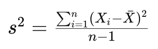
where barred X is the mean of the dataset. The division by n-1 instead of n is done to correct for bias in the estimation of the population variance when using a sample. This correction is known as Bessel’s correction and helps to provide an unbiased estimate of the population variance based on the sample data.
If we now assume our datapoints to be presented in an n-dimensional vector, X² will result in an nxn matrix. This is known as the sample covariance matrix. The covariance matrix is hence defined as

With this, we can implement this in Pytorch using its built-in PCA functions:
import torch
from sklearn.decomposition import PCA
from sklearn.datasets import make_blobs
import matplotlib.pyplot as plt

# Create synthetic data
data, labels = make_blobs(n_samples=100, n_features=2, centers=1,random_state=15)

# Convert NumPy array to PyTorch tensor
tensor_data = torch.from_numpy(data).float()

# Compute the mean of the data
mean = torch.mean(tensor_data, dim=0)

# Center the data by subtracting the mean
centered_data = tensor_data - mean

# Compute the covariance matrix
covariance_matrix = torch.mm(centered_data.t(), centered_data) / (tensor_data.size(0) - 1)

# Perform eigendecomposition of the covariance matrix
eigenvalues, eigenvectors = torch.linalg.eig(covariance_matrix)

# Sort eigenvalues and corresponding eigenvectors
sorted_indices = torch.argsort(eigenvalues.real, descending=True)
eigenvalues = eigenvalues[sorted_indices]
eigenvectors = eigenvectors[:, sorted_indices].to(centered_data.dtype)

# Pick the first two components
principal_components = eigenvectors[:, :2]*eigenvalues[:2].real

# Plot the original data with eigenvectors
plt.scatter(tensor_data[:, 0], tensor_data[:, 1], c=labels, cmap='viridis', label='Original Data')
plt.axis('equal')
plt.arrow(mean[0], mean[1], principal_components[0, 0], principal_components[1, 0], color='red', label='PC1')
plt.arrow(mean[0], mean[1], principal_components[0, 1], principal_components[1, 1], color='blue', label='PC2')

# Plot an ellipse around the Eigenvectors
angle = torch.atan2(principal_components[1,1],principal_components[0,1]).detach().numpy()/3.1415*180
ellipse=pat.Ellipse((mean[0].detach(), mean[1].detach()), 2*torch.norm(principal_components[:,1]), 2*torch.norm(principal_components[:,0]), angle=angle, fill=False)
ax = plt.gca()
ax.add_patch(ellipse)

plt.legend()
plt.show()
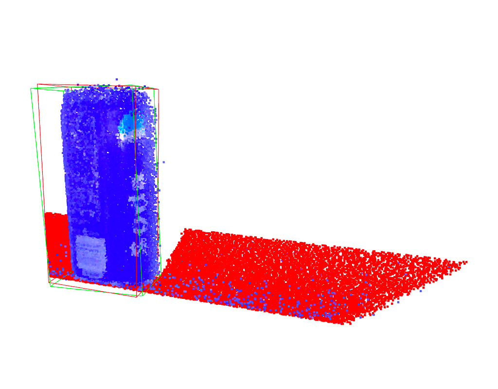
Note that the output of the PCA function is not necessarily sorted by the largest Eigenvalue. We are using the real part of each Eigenvalue for this and plot the resulting Eigenvectors below. Also note that we multiply each Eigenvector with the real part of its Eigenvalue to scale them.
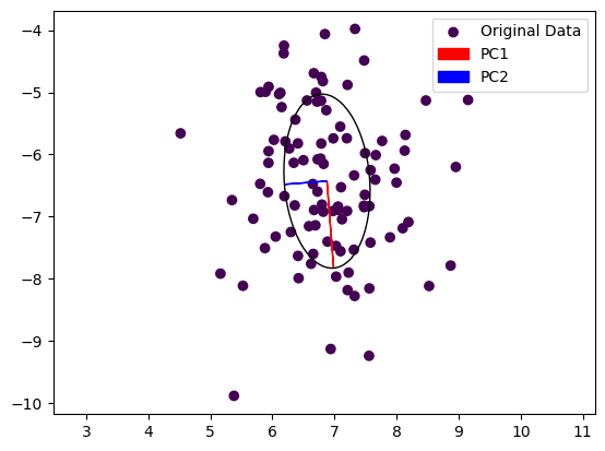
We can see that the first principal component, the dominant Eigenvector, is aligned with the longer axes of our random point cloud, whereas the second Eigenvector is aligned with the shorter axis. In a robotic application, we could now grasp this object by turning our gripper so that it is parallel to PC1 and close it along PC2. This of course works also in 3D, allowing us to also adjust the gripper’s pitch.
But what does the PCA function actually do? In practice, PCA is implemented using a singular value decomposition as solving the deterministic equation det(A−λI)=0 to find the Eigenvalues λ of a matrix A and hence computing the Eigenvectors might be infeasible. We will instead look at a simple numerical method to build some intution.
The power iteration method is a simple and intuitive algorithm used to find the dominant eigenvector and eigenvalue of a square matrix. It’s particularly useful in the context of data science and machine learning when dealing with large, high-dimensional datasets, if only the first few Eigenvectors are needed.
An eigenvector is a non-zero vector that, when multiplied by a square matrix, results in a scaled version of the same vector. In other words, if A is a square matrix and v is a non-zero vector, then v is an eigenvector of A if there exists a scalar λ (called the eigenvalue) such that:
Av=λv
Here:
In other words, the matrix is reduced to a single number when multiplying its Eigenvectors. The power iteration method takes advantage of this by simply multiplying a random vector with A over and over again, and normalizing it.
Here’s a breakdown of the power iteration method:
And here is the code:
def power_iteration(A, num_iterations=100):
    # 1. Initialize a random vector
    v = torch.randn(A.shape[1], 1, dtype=A.dtype)

    for _ in range(num_iterations):
        # 2. Multiply matrix by current vector and normalize
        v = torch.matmul(A, v)
        v /= torch.norm(v)
        # 3. Repeat

    # Compute the dominant eigenvalue
    eigenvalue = torch.matmul(torch.matmul(v.t(), A), v)

    return eigenvalue.item(), v.squeeze()

# Example: find the dominant eigenvector and Eigenvalue of a covariance matrix
dominant_eigenvalue, dominant_eigenvector = power_iteration(covariance_matrix)
In essence, the power iteration method leverages the repeated application of the matrix to a vector, causing the vector to align with the dominant eigenvector. It’s a straightforward and computationally efficient method, especially useful for large datasets where direct computation of eigenvectors may be impractical.
Power iteration finds only the dominant eigenvector and eigenvalue. In order to find the next Eigenvector, we need to flatten the matrix. For this, we subtract the contribution of an Eigenvector from the original matrix:
A′=A−λvv^t
or in code:
def deflate_matrix(A, eigenvalue, eigenvector):
    deflated_matrix = A - eigenvalue * torch.matmul(eigenvector, eigenvector.t())
    return deflated_matrix
The purpose of obtaining a deflated matrix is to facilitate the iterative computation of subsequent eigenvalues and eigenvectors. After finding the first eigenvalue-eigenvector pair, you can use the deflated matrix to find the next one, and so on.
The result of this approach is not necessarily orthogonal, however. Gram-Schmidt orthogonalization is a process in linear algebra used to transform a set of linearly independent vectors into a set of orthogonal (perpendicular) vectors. This method is named after mathematicians Jørgen Gram and Erhard Schmidt and is particularly useful when working with non-orthogonal bases.
def gram_schmidt(v, u):
    # Gram-Schmidt orthogonalization
    projection = torch.matmul(u.t(), v) / torch.matmul(u.t(), u)
    v = v.squeeze(-1) - projection * u
    return v
We can now add Gram-Schmidt Orthogonalization to the Power Method and compute both the Dominant and the Second Eigenvector:
# Power iteration to find dominant eigenvector
dominant_eigenvalue, dominant_eigenvector = power_iteration(covariance_matrix)

deflated_matrix = deflate_matrix(covariance_matrix, dominant_eigenvalue, dominant_eigenvector)
second_eigenvector = deflated_matrix[:, 0].view(-1, 1)


# Power iteration to find the second eigenvector
for _ in range(100):
    second_eigenvector = torch.matmul(covariance_matrix, second_eigenvector)
    second_eigenvector /= torch.norm(second_eigenvector)
    # Orthogonalize with respect to the first eigenvector
    second_eigenvector = gram_schmidt(second_eigenvector, dominant_eigenvector)

second_eigenvalue = torch.matmul(torch.matmul(second_eigenvector.t(), covariance_matrix), second_eigenvector)
We can now plot the Eigenvectors computed with either method next to each other:
# Scale Eigenvectors by Eigenvalues
dominant_eigenvector *= dominant_eigenvalue
second_eigenvector *= second_eigenvalue

# Plot the original data with eigenvectors computed either way
plt.scatter(tensor_data[:, 0], tensor_data[:, 1], c=labels, cmap='viridis', label='Original Data')
plt.axis('equal')
plt.arrow(mean[0], mean[1], principal_components[0, 0], principal_components[1, 0], color='red', label='PC1')
plt.arrow(mean[0], mean[1], principal_components[0, 1], principal_components[1, 1], color='blue', label='PC2')
plt.arrow(mean[0], mean[1], dominant_eigenvector[0], dominant_eigenvector[1], color='orange', label='approx1')
plt.arrow(mean[0], mean[1], second_eigenvector[0], second_eigenvector[1], color='purple', label='approx2')
plt.legend()
plt.show()
…and the result is:
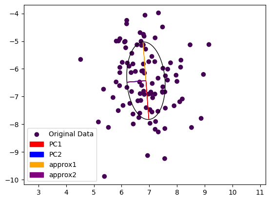
Note that the second Eigenvector coming from power iteration (purple) is painted over the second Eigenvector computed by the exact method (blue). The dominant Eigenvector from power iteration (yellow) is pointing in the other direction then the exact dominant Eigenvector (red). This is not really surprising, as we started from a random vector during power iteration and the result could come out either way.
We presented a simple numerical method to compute the Eigenvectors of a Covariance Matrix to derive the Principal Components of a dataset, shedding some light on the properties of Eigenvectors and Eigenvalues.
Understanding Principal Component Analysis in PyTorch was originally published in Towards Data Science on Medium, where people are continuing the conversation by highlighting and responding to this story.
Originally appeared here:
Understanding Principal Component Analysis in PyTorch
Go Here to Read this Fast! Understanding Principal Component Analysis in PyTorch