Category: AI

How to Forecast Time Series Data Using any Supervised Learning Model

Featurizing time series data into a standard tabular format for classical ML models and improving accuracy using AutoML

This article delves into enhancing the process of forecasting daily energy consumption levels by transforming a time series dataset into a tabular format using open-source libraries. We explore the application of a popular multiclass classification model and leverage AutoML with Cleanlab Studio to significantly boost our out-of-sample accuracy.

The key takeaway from this article is that we can utilize more general methods to model a time series dataset by converting it to a tabular structure, and even find improvements in trying to predict this time series data.

Take a Snapshot

At a high level we will:

• Establish a baseline accuracy by fitting a Prophet forecasting model on our time series data
• Convert our time series data into a tabular format by using open-source featurization libraries and then will show that can outperform our Prophet model with a standard multiclass classification (Gradient Boosting) approach by a 67% reduction in prediction error (increase by 38% raw percentage points in out-of-sample accuracy).
• Use an AutoML solution for multiclass classification resulted in a 42% reduction in prediction error (increase by 8% in raw percentage points in out-of-sample accuracy) compared to our Gradient Boosting model and resulted in a 81% reduction in prediction error (increase by 46% in raw percentage points in out-of-sample accuracy) compared to our Prophet forecasting model.

To run the code demonstrated in this article, here’s the full notebook.

Examine the Data

You can download the dataset here.

The data represents PJM hourly energy consumption (in megawatts) on an hourly basis. PJM Interconnection LLC (PJM) is a regional transmission organization (RTO) in the United States. It is part of the Eastern Interconnection grid operating an electric transmission system serving many states.

Let’s take a look at our dataset. The data includes one datetime column (object type), and the Megawatt Energy Consumption (float64) type) column we are trying to forecast as a discrete variable (corresponding to the quartile of hourly energy consumption levels). Our aim is to train a time series forecasting model to be able to forecast the tomorrow’s daily energy consumption level falling into 1 of 4 levels: low , below average , above average or high (these levels were determined based on quartiles of the overall daily consumption distribution). We first demonstrate how to apply time-series forecasting methods like Prophet to this problem, but these are restricted to certain types of ML models suitable for time-series data. Next we demonstrate how to reframe this problem into a standard multiclass classification problem that we can apply any machine learning model to, and show how we can obtain superior forecasts by using powerful supervised ML.

We first convert this data into a average energy consumption at a daily level and rename the columns to the format that the Prophet forecasting model expects. These real-valued daily energy consumption levels are converted into quartiles, which is the value we are trying to predict. Our training data is shown below along with the quartile each daily energy consumption level falls into. The quartiles are computed using training data to prevent data leakage.

We then show the test data below, which is the data we are evaluating our forecasting results against.

We then show the test data below, which is the data we are evaluating our forecasting results against.

Train and Evaluate Prophet Forecasting Model

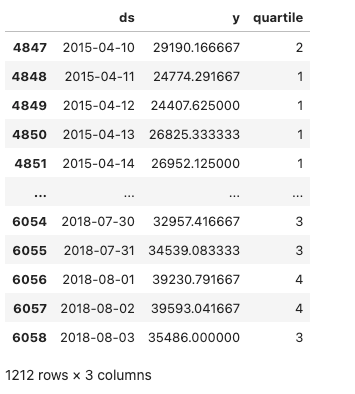
As seen in the images above, we will use a date cutoff of 2015-04-09 to end the range of our training data and start our test data at 2015-04-10 . We compute quartile thresholds of our daily energy consumption using ONLY training data. This avoids data leakage – using out-of-sample data that is available only in the future.

Next, we will forecast the daily PJME energy consumption level (in MW) for the duration of our test data and represent the forecasted values as a discrete variable. This variable represents which quartile the daily energy consumption level falls into, represented categorically as 1 (low), 2 (below average), 3 (above average), or 4 (high). For evaluation, we are going to use the accuracy_score function from scikit-learn to evaluate the performance of our models. Since we are formulating the problem this way, we are able to evaluate our model’s next-day forecasts (and compare future models) using classification accuracy.

import numpy as np
from prophet import Prophet
from sklearn.metrics import accuracy_score

# Initialize model and train it on training data
model = Prophet()
model.fit(train_df)

# Create a dataframe for future predictions covering the test period
future = model.make_future_dataframe(periods=len(test_df), freq='D')
forecast = model.predict(future)

# Categorize forecasted daily values into quartiles based on the thresholds
forecast['quartile'] = pd.cut(forecast['yhat'], bins = [-np.inf] + list(quartiles) + [np.inf], labels=[1, 2, 3, 4])

# Extract the forecasted quartiles for the test period
forecasted_quartiles = forecast.iloc[-len(test_df):]['quartile'].astype(int)

# Categorize actual daily values in the test set into quartiles
test_df['quartile'] = pd.cut(test_df['y'], bins=[-np.inf] + list(quartiles) + [np.inf], labels=[1, 2, 3, 4])
actual_test_quartiles = test_df['quartile'].astype(int)

# Calculate the evaluation metrics
accuracy = accuracy_score(actual_test_quartiles, forecasted_quartiles)

# Print the evaluation metrics
print(f'Accuracy: {accuracy:.4f}')
>>> 0.4249

The out-of-sample accuracy is quite poor at 43%. By modelling our time series this way, we limit ourselves to only use time series forecasting models (a limited subset of possible ML models). In the next section, we consider how we can more flexibly model this data by transforming the time-series into a standard tabular dataset via appropriate featurization. Once the time-series has been transformed into a standard tabular dataset, we’re able to employ any supervised ML model for forecasting this daily energy consumption data.

Convert time series data to tabular data through featurization

Now we convert the time series data into a tabular format and featurize the data using the open source libraries sktime, tsfresh, and tsfel. By employing libraries like these, we can extract a wide array of features that capture underlying patterns and characteristics of the time series data. This includes statistical, temporal, and possibly spectral features, which provide a comprehensive snapshot of the data’s behavior over time. By breaking down time series into individual features, it becomes easier to understand how different aspects of the data influence the target variable.

TSFreshFeatureExtractor is a feature extraction tool from the sktime library that leverages the capabilities of tsfresh to extract relevant features from time series data. tsfresh is designed to automatically calculate a vast number of time series characteristics, which can be highly beneficial for understanding complex temporal dynamics. For our use case, we make use of the minimal and essential set of features from our TSFreshFeatureExtractor to featurize our data.

tsfel, or Time Series Feature Extraction Library, offers a comprehensive suite of tools for extracting features from time series data. We make use of a predefined config that allows for a rich set of features (e.g., statistical, temporal, spectral) to be constructed from the energy consumption time series data, capturing a wide range of characteristics that might be relevant for our classification task.

import tsfel
from sktime.transformations.panel.tsfresh import TSFreshFeatureExtractor

# Define tsfresh feature extractor
tsfresh_trafo = TSFreshFeatureExtractor(default_fc_parameters="minimal")

# Transform the training data using the feature extractor
X_train_transformed = tsfresh_trafo.fit_transform(X_train)

# Transform the test data using the same feature extractor
X_test_transformed = tsfresh_trafo.transform(X_test)

# Retrieves a pre-defined feature configuration file to extract all available features
cfg = tsfel.get_features_by_domain()

# Function to compute tsfel features per day
def compute_features(group):
    # TSFEL expects a DataFrame with the data in columns, so we transpose the input group
    features = tsfel.time_series_features_extractor(cfg, group, fs=1, verbose=0)
    return features


# Group by the 'day' level of the index and apply the feature computation
train_features_per_day = X_train.groupby(level='Date').apply(compute_features).reset_index(drop=True)
test_features_per_day = X_test.groupby(level='Date').apply(compute_features).reset_index(drop=True)

# Combine each featurization into a set of combined features for our train/test data
train_combined_df = pd.concat([X_train_transformed, train_features_per_day], axis=1)
test_combined_df = pd.concat([X_test_transformed, test_features_per_day], axis=1)

Next, we clean our dataset by removing features that showed a high correlation (above 0.8) with our target variable — average daily energy consumption levels — and those with null correlations. High correlation features can lead to overfitting, where the model performs well on training data but poorly on unseen data. Null-correlated features, on the other hand, provide no value as they lack a definable relationship with the target.

By excluding these features, we aim to improve model generalizability and ensure that our predictions are based on a balanced and meaningful set of data inputs.

# Filter out features that are highly correlated with our target variable
column_of_interest = "PJME_MW__mean"
train_corr_matrix = train_combined_df.corr()
train_corr_with_interest = train_corr_matrix[column_of_interest]
null_corrs = pd.Series(train_corr_with_interest.isnull())
false_features = null_corrs[null_corrs].index.tolist()

columns_to_exclude = list(set(train_corr_with_interest[abs(train_corr_with_interest) > 0.8].index.tolist() + false_features))
columns_to_exclude.remove(column_of_interest)

# Filtered DataFrame excluding columns with high correlation to the column of interest
X_train_transformed = train_combined_df.drop(columns=columns_to_exclude)
X_test_transformed = test_combined_df.drop(columns=columns_to_exclude)

If we look at the first several rows of the training data now, this is a snapshot of what it looks like. We now have 73 features that were added from the time series featurization libraries we used. The label we are going to predict based on these features is the next day’s energy consumption level.

It’s important to note that we used a best practice of applying the featurization process separately for training and test data to avoid data leakage (and the held-out test data are our most recent observations).

Also, we compute our discrete quartile value (using the quartiles we originally defined) using the following code to obtain our train/test energy labels, which is what our y_labels are.

# Define a function to classify each value into a quartile
def classify_into_quartile(value):
    if value < quartiles[0]:
        return 1  
    elif value < quartiles[1]:
        return 2  
    elif value < quartiles[2]:
        return 3  
    else:
        return 4  

y_train = X_train_transformed["PJME_MW__mean"].rename("daily_energy_level")
X_train_transformed.drop("PJME_MW__mean", inplace=True, axis=1)

y_test = X_test_transformed["PJME_MW__mean"].rename("daily_energy_level")
X_test_transformed.drop("PJME_MW__mean", inplace=True, axis=1)

energy_levels_train = y_train.apply(classify_into_quartile)
energy_levels_test = y_test.apply(classify_into_quartile)

Train and Evaluate GradientBoostingClassifier Model on featurized tabular data

Using our featurized tabular dataset, we can apply any supervised ML model to predict future energy consumption levels. Here we’ll use a Gradient Boosting Classifier (GBC) model, the weapon of choice for most data scientists operating on tabular data.

Our GBC model is instantiated from the sklearn.ensemble module and configured with specific hyperparameters to optimize its performance and avoid overfitting.

from sklearn.ensemble import GradientBoostingClassifier

gbc = GradientBoostingClassifier(
    n_estimators=150,
    learning_rate=0.1,
    max_depth=4,
    min_samples_leaf=20,
    max_features='sqrt',
    subsample=0.8,
    random_state=42
)

gbc.fit(X_train_transformed, energy_levels_train)


y_pred_gbc = gbc.predict(X_test_transformed)
gbc_accuracy = accuracy_score(energy_levels_test, y_pred_gbc)
print(f'Accuracy: {gbc_accuracy:.4f}')
>>> 0.8075

The out-of-sample accuracy of 81% is considerably better than our prior Prophet model results.

Using AutoML to streamline things

Now that we’ve seen how to featurize the time-series problem and the benefits of applying powerful ML models like Gradient Boosting, a natural question emerges: Which supervised ML model should we apply? Of course, we could experiment with many models, tune their hyperparameters, and ensemble them together. An easier solution is to let AutoML handle all of this for us.

Here we’ll use a simple AutoML solution provided in Cleanlab Studio, which involves zero configuration. We just provide our tabular dataset, and the platform automatically trains many types of supervised ML models (including Gradient Boosting among others), tunes their hyperparameters, and determines which models are best to combine into a single predictor. Here’s all the code needed to train and deploy an AutoML supervised classifier:

from cleanlab_studio import Studio

studio = Studio()
studio.create_project(
    dataset_id=energy_forecasting_dataset,
    project_name="ENERGY-LEVEL-FORECASTING",
    modality="tabular",
    task_type="multi-class",
    model_type="regular",
    label_column="daily_energy_level",
)

model = studio.get_model(energy_forecasting_model)
y_pred_automl = model.predict(test_data, return_pred_proba=True)

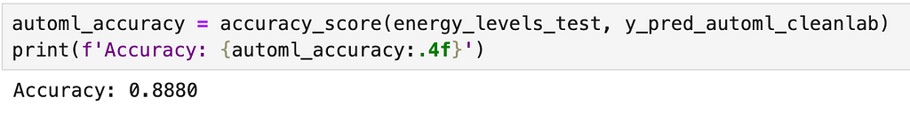
Below we can see model evaluation estimates in the AutoML platform, showing all of the different types of ML models that were automatically fit and evaluated (including multiple Gradient Boosting models), as well as an ensemble predictor constructed by optimally combining their predictions.

After running inference on our test data to obtain the next-day energy consumption level predictions, we see the test accuracy is 89%, a 8% raw percentage points improvement compared to our previous Gradient Boosting approach.

Conclusion

For our PJM daily energy consumption data, we found that transforming the data into a tabular format and featurizing it achieved a 67% reduction in prediction error (increase by 38% in raw percentage points in out-of-sample accuracy) compared to our baseline accuracy established with our Prophet forecasting model.

We also tried an easy AutoML approach for multiclass classification, which resulted in a 42% reduction in prediction error (increase by 8% in raw percentage points in out-of-sample accuracy) compared to our Gradient Boosting model and resulted in a 81% reduction in prediction error (increase by 46% in raw percentage points in out-of-sample accuracy) compared to our Prophet forecasting model.

By taking approaches like those illustrated above to model a time series dataset beyond the constrained approach of only considering forecasting methods, we can apply more general supervised ML techniques and achieve better results for certain types of forecasting problems.

Unless otherwise noted, all images are by the author.

---

How to Forecast Time Series Data using any Supervised Learning Model was originally published in Towards Data Science on Medium, where people are continuing the conversation by highlighting and responding to this story.

Posted by Long Zhao, Senior Research Scientist, and Ting Liu, Senior Staff Software Engineer, Google Research

An astounding number of videos are available on the Web, covering a variety of content from everyday moments people share to historical moments to scientific observations, each of which contains a unique record of the world. The right tools could help researchers analyze these videos, transforming how we understand the world around us.

Videos offer dynamic visual content far more rich than static images, capturing movement, changes, and dynamic relationships between entities. Analyzing this complexity, along with the immense diversity of publicly available video data, demands models that go beyond traditional image understanding. Consequently, many of the approaches that best perform on video understanding still rely on specialized models tailor-made for particular tasks. Recently, there has been exciting progress in this area using video foundation models (ViFMs), such as VideoCLIP, InternVideo, VideoCoCa, and UMT). However, building a ViFM that handles the sheer diversity of video data remains a challenge.

With the goal of building a single model for general-purpose video understanding, we introduced “VideoPrism: A Foundational Visual Encoder for Video Understanding”. VideoPrism is a ViFM designed to handle a wide spectrum of video understanding tasks, including classification, localization, retrieval, captioning, and question answering (QA). We propose innovations in both the pre-training data as well as the modeling strategy. We pre-train VideoPrism on a massive and diverse dataset: 36 million high-quality video-text pairs and 582 million video clips with noisy or machine-generated parallel text. Our pre-training approach is designed for this hybrid data, to learn both from video-text pairs and the videos themselves. VideoPrism is incredibly easy to adapt to new video understanding challenges, and achieves state-of-the-art performance using a single frozen model.

VideoPrism is a general-purpose video encoder that enables state-of-the-art results over a wide spectrum of video understanding tasks, including classification, localization, retrieval, captioning, and question answering, by producing video representations from a single frozen model.

Pre-training data

A powerful ViFM needs a very large collection of videos on which to train — similar to other foundation models (FMs), such as those for large language models (LLMs). Ideally, we would want the pre-training data to be a representative sample of all the videos in the world. While naturally most of these videos do not have perfect captions or descriptions, even imperfect text can provide useful information about the semantic content of the video.

To give our model the best possible starting point, we put together a massive pre-training corpus consisting of several public and private datasets, including YT-Temporal-180M, InternVid, VideoCC, WTS-70M, etc. This includes 36 million carefully selected videos with high-quality captions, along with an additional 582 million clips with varying levels of noisy text (like auto-generated transcripts). To our knowledge, this is the largest and most diverse video training corpus of its kind.

Statistics on the video-text pre-training data. The large variations of the CLIP similarity scores (the higher, the better) demonstrate the diverse caption quality of our pre-training data, which is a byproduct of the various ways used to harvest the text.

Two-stage training

The VideoPrism model architecture stems from the standard vision transformer (ViT) with a factorized design that sequentially encodes spatial and temporal information following ViViT. Our training approach leverages both the high-quality video-text data and the video data with noisy text mentioned above. To start, we use contrastive learning (an approach that minimizes the distance between positive video-text pairs while maximizing the distance between negative video-text pairs) to teach our model to match videos with their own text descriptions, including imperfect ones. This builds a foundation for matching semantic language content to visual content.

After video-text contrastive training, we leverage the collection of videos without text descriptions. Here, we build on the masked video modeling framework to predict masked patches in a video, with a few improvements. We train the model to predict both the video-level global embedding and token-wise embeddings from the first-stage model to effectively leverage the knowledge acquired in that stage. We then randomly shuffle the predicted tokens to prevent the model from learning shortcuts.

What is unique about VideoPrism’s setup is that we use two complementary pre-training signals: text descriptions and the visual content within a video. Text descriptions often focus on what things look like, while the video content provides information about movement and visual dynamics. This enables VideoPrism to excel in tasks that demand an understanding of both appearance and motion.

Results

We conducted extensive evaluation on VideoPrism across four broad categories of video understanding tasks, including video classification and localization, video-text retrieval, video captioning, question answering, and scientific video understanding. VideoPrism achieves state-of-the-art performance on 30 out of 33 video understanding benchmarks — all with minimal adaptation of a single, frozen model.

VideoPrism compared to the previous best-performing FMs.

Classification and localization

We evaluate VideoPrism on an existing large-scale video understanding benchmark (VideoGLUE) covering classification and localization tasks. We found that (1) VideoPrism outperforms all of the other state-of-the-art FMs, and (2) no other single model consistently came in second place. This tells us that VideoPrism has learned to effectively pack a variety of video signals into one encoder — from semantics at different granularities to appearance and motion cues — and it works well across a variety of video sources.

VideoPrism outperforms state-of-the-art approaches (including CLIP, VATT, InternVideo, and UMT) on the video understanding benchmark. In this plot, we show the absolute score differences compared with the previous best model to highlight the relative improvements of VideoPrism. On Charades, ActivityNet, AVA, and AVA-K, we use mean average precision (mAP) as the evaluation metric. On the other datasets, we report top-1 accuracy.

Combining with LLMs

We further explore combining VideoPrism with LLMs to unlock its ability to handle various video-language tasks. In particular, when paired with a text encoder (following LiT) or a language decoder (such as PaLM-2), VideoPrism can be utilized for video-text retrieval, video captioning, and video QA tasks. We compare the combined models on a broad and challenging set of vision-language benchmarks. VideoPrism sets the new state of the art on most benchmarks. From the visual results, we find that VideoPrism is capable of understanding complex motions and appearances in videos (e.g., the model can recognize the different colors of spinning objects on the window in the visual examples below). These results demonstrate that VideoPrism is strongly compatible with language models.

VideoPrism achieves competitive results compared with state-of-the-art approaches (including VideoCoCa, UMT and Flamingo) on multiple video-text retrieval (top) and video captioning and video QA (bottom) benchmarks. We also show the absolute score differences compared with the previous best model to highlight the relative improvements of VideoPrism. We report the Recall@1 on MASRVTT, VATEX, and ActivityNet, CIDEr score on MSRVTT-Cap, VATEX-Cap, and YouCook2, top-1 accuracy on MSRVTT-QA and MSVD-QA, and WUPS index on NExT-QA.

We show qualitative results using VideoPrism with a text encoder for video-text retrieval (first row) and adapted to a language decoder for video QA (second and third row). For video-text retrieval examples, the blue bars indicate the embedding similarities between the videos and the text queries.

Scientific applications

Finally, we tested VideoPrism on datasets used by scientists across domains, including fields such as ethology, behavioral neuroscience, and ecology. These datasets typically require domain expertise to annotate, for which we leverage existing scientific datasets open-sourced by the community including Fly vs. Fly, CalMS21, ChimpACT, and KABR. VideoPrism not only performs exceptionally well, but actually surpasses models designed specifically for those tasks. This suggests tools like VideoPrism have the potential to transform how scientists analyze video data across different fields.

VideoPrism outperforms the domain experts on various scientific benchmarks. We show the absolute score differences to highlight the relative improvements of VideoPrism. We report mean average precision (mAP) for all datasets, except for KABR which uses class-averaged top-1 accuracy.

Conclusion

With VideoPrism, we introduce a powerful and versatile video encoder that sets a new standard for general-purpose video understanding. Our emphasis on both building a massive and varied pre-training dataset and innovative modeling techniques has been validated through our extensive evaluations. Not only does VideoPrism consistently outperform strong baselines, but its unique ability to generalize positions it well for tackling an array of real-world applications. Because of its potential broad use, we are committed to continuing further responsible research in this space, guided by our AI Principles. We hope VideoPrism paves the way for future breakthroughs at the intersection of AI and video analysis, helping to realize the potential of ViFMs across domains such as scientific discovery, education, and healthcare.

Acknowledgements

This blog post is made on behalf of all the VideoPrism authors: Long Zhao, Nitesh B. Gundavarapu, Liangzhe Yuan, Hao Zhou, Shen Yan, Jennifer J. Sun, Luke Friedman, Rui Qian, Tobias Weyand, Yue Zhao, Rachel Hornung, Florian Schroff, Ming-Hsuan Yang, David A. Ross, Huisheng Wang, Hartwig Adam, Mikhail Sirotenko, Ting Liu, and Boqing Gong. We sincerely thank David Hendon for their product management efforts, and Alex Siegman, Ramya Ganeshan, and Victor Gomes for their program and resource management efforts. We also thank Hassan Akbari, Sherry Ben, Yoni Ben-Meshulam, Chun-Te Chu, Sam Clearwater, Yin Cui, Ilya Figotin, Anja Hauth, Sergey Ioffe, Xuhui Jia, Yeqing Li, Lu Jiang, Zu Kim, Dan Kondratyuk, Bill Mark, Arsha Nagrani, Caroline Pantofaru, Sushant Prakash, Cordelia Schmid, Bryan Seybold, Mojtaba Seyedhosseini, Amanda Sadler, Rif A. Saurous, Rachel Stigler, Paul Voigtlaender, Pingmei Xu, Chaochao Yan, Xuan Yang, and Yukun Zhu for the discussions, support, and feedback that greatly contributed to this work. We are grateful to Jay Yagnik, Rahul Sukthankar, and Tomas Izo for their enthusiastic support for this project. Lastly, we thank Tom Small, Jennifer J. Sun, Hao Zhou, Nitesh B. Gundavarapu, Luke Friedman, and Mikhail Sirotenko for the tremendous help with making this blog post.

Carbon Footprint of LLM Fine Tuning — A Case Study

I got surprising results when I measured the carbon emissions from instruction fine tuning an LLM

I recently LoRA fine-tuned a Danish LLM called Munin-7b-alpha on an instruction fine tuning dataset called SkoleGPT-instruct. During the fine tuning procedure, I measured the energy consumption and computed the carbon footprint. In this article, I present the surprising results. You can find the model here.

Introduction

Munin-7b-alpha is a pre-trained model (or a so-called foundation model), which has been trained solely to generate text. To make them suitable for a chat setup, pre-trained models need to be good at following instructions, which requires a subsequent training step called instruction fine tuning.

As opposed to pre-training, which requires massive amounts of unlabeled text data on which the model trains in a self-supervised fashion, instruction fine tuning requires a relatively modest amount of data, which in turn must be carefully curated and annotated.

It is a fune-tuning procedure that I report on in this article.

Set up a local LLM on CPU with chat UI in 15 minutes

Methodology

The Munin-7b-alpha has 7 billion parameters and the instruction dataset that I used consists of 21,300 samples. That is, 21,300 examples of a prompt and a good answer.

Using an slightly adapted version of this fantastic model fine tuning notebook, I trained a LoRA for 1 epoch, i.e. I showed the model each sample once.

LoRA – low rank adaptation – is an efficient fine tuning technique for adapting LLMs to specific tasks. Hugging Face provides a succinct description of the technique:

“Low-Rank Adaptation (LoRA) is a PEFT [parameter efficient fine tuning] method that decomposes a large matrix into two smaller low-rank matrices in the attention layers. This drastically reduces the number of parameters that need to be fine-tuned.”

The model trained on a single Nvidia RTX A4000 GPU, which is a consumer grade GPU with 16 GB memory – just enough memory for LoRA fine tuning of this model.

I measured energy consumption with the Python package CodeCarbon. CodeCarbon is an extremely light weight and easy-to-use package that let’s you measure the energy consumption of a Python script, function or method with just two lines of code. Read more about how to use it here:

How to estimate and reduce the carbon footprint of machine learning models

Aside from energy consumption, CodeCarbon also estimates the carbon footprint of the energy your computing procedure consumes, but I found the numbers to appear inaccurate. This is likely because CodeCarbon uses a hardcoded average carbon intensity (CO2e per produced KWh) of your geographic region and not an near real time carbon intensity. So I went to a website called Energi Data Service, which lets you download fine grained electricity emissions data from the Danish grid. By multiplying the energy consumption measurements obtained with CodeCarbon by the carbon intensity of electricity in the grid during the hours the model trained, I obtained the carbon footprint of the training.

ChatGPT’s energy use per query

Results

The fine tuning process took just shy of 4 hours and consumed a total of 0.694 KWh – the combined GPU, CPU and RAM consumption as per estimates produced with the Python package CodeCarbon.

During the hours the model trained, the average C02e emissions per produced KWh was 82.5 g as per Energi Data Service (license: “The Licensor grants you a worldwide, free, non-exclusive and otherwise unrestricted licence to use the Data” [1]).

Thus, the fine tuning emitted a minuscule 57 grams of CO2e (0.694 KWh * 82.5 g).

For comparison, the average Dane emits 11 TONS CO2e per year.

Generating a single image with generative AI has been found in a research study to consume 2.9 Wh on average [2]. So for the amount of energy it took to instruction fine-tune the LLM, you can generate a mere 239 images.

If you’re wondering if such a short and efficient fine-tuning procedure yielded a better model, the answer is a clear “yes”:

According to the ScandEval leader board on natural language generation, the pre-trained model scores an average of 43.44 on Danish tasks and the fine tuned model scores an average of 47.55. A gain of 9.45 percent. As of this writing, that’s the difference between a 5th place and a 7th place on the leader board.

How to make a PyTorch Transformer for time series forecasting

Discussion

It’s surprising to me that it did not require more compute, energy, and emissions to perform the fine tuning.

I expect my findings to scale linearly with the amount of samples if holding other variables constant (e.g. using a similar GPU, training method etc.). I.e. if you fine tune on twice the amount of samples, or for double the number of epochs, I expect the energy consumption to double.

The energy consumption will likely be significantly higher for a 70 billion parameter model, thus leading to higher emissions, but emissions would probably still very modest in the grand scheme of things.

Further, the energy consumption would likely be higher if I hadn’t used LoRA.

Conclusion

Using the instruction fine-tuning technique LoRA is indeed efficient—both in terms of how long it takes, how much compute (eg GPU RAM) you need, and how much carbon it emits.

Instruction fine tuning a 7B LLM with LoRA on 21,300 samples for one epoch took four hours and emitted 57 gram CO2e—a tiny amount.

That’s it! I hope you enjoyed the story. Let me know what you think!

Get the benefits of Medium and support my writing by signing up for a Medium membership HERE.

Follow me for more on AI and sustainability and subscribe to get my stories via email when I publish.

I also sometimes write about time series forecasting.

And feel free to connect on LinkedIn.

References

[1] https://www.energidataservice.dk/Conditions_for_use_of_Danish_public_sector_data-License_for_use_of_data_in_ED.pdf

[2] “Power Hungry Processing: Watts Driving the Cost of AI Deployment?” by Luccioni et al

---

Carbon footprint of LLM fine tuning — a case study was originally published in Towards Data Science on Medium, where people are continuing the conversation by highlighting and responding to this story.

A guide on accelerating inference performance

Intro

Open-source large language models have lived up to the hype. Many companies that use GPT-3.5 or GPT-4 in production have realized that these models are simply not scalable from a cost perspective. Because of this, enterprises are looking for good open-source alternatives. Recent models like Mixtral and Llama 2 have shown stellar results when it comes to output quality. But, scaling these models to support thousands of concurrent users still remains a challenge.

While frameworks such as vLLM and TGI are a great starting point for boosting inference, they lack some optimizations, making it difficult to scale them in production.

This is where TensorRT-LLM comes in. TensorRT-LLM is an open-source framework designed by Nvidia to boost the performance of large language models in a production environment. Most of the big shots such as Anthropic, OpenAI, Anyscale, etc. are already using this framework to serve LLMs to millions of users.

Understanding TensorRT-LLM

Unlike other inference techniques, TensorRT LLM does not serve the model using raw weights. Instead, it compiles the model and optimizes the kernels to enable efficient serving on an Nvidia GPU. The performance benefits of running a compiled model are far greater than running it raw. This is one of the main reasons why TensorRT LLM is blazing fast.

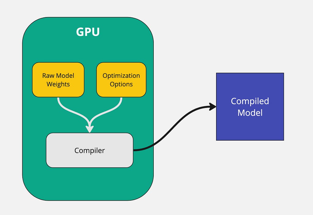
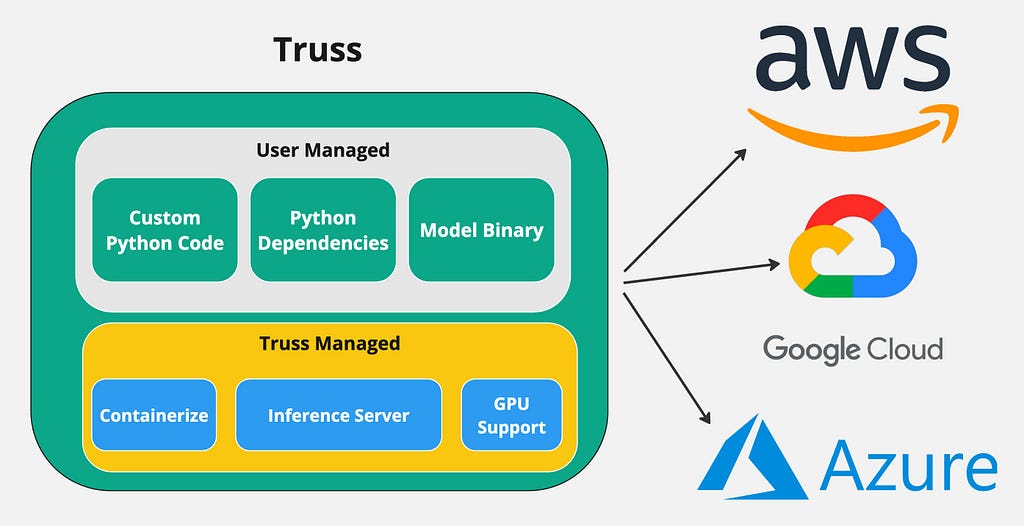
The raw model weights along with optimization options such as quantization level, tensor parallelism, pipeline parallelism, etc. get passed to the compiler. The compiler then takes that information and outputs a model binary that is optimized for the specific GPU.

An important thing to note is that the entire model compilation process MUST take place on a GPU. The compiled model that gets generated is optimized specifically on the GPU that it is run on. For example, if you compile the model on a A40 GPU, you won’t be able to run it on an A100 GPU. So whatever GPU is used during compilation, the same GPU must get used for inference.

TensorRT LLM does not support all large language models out of the box. The reason is that each model architecture is different and TensorRT does deep graph level optimizations. With that being said, most of the popular models such as Mistral, Llama, and Qwen are supported. If you’re curious about the full list of supported models you can check the TensorRT LLM Github repository.

Benefits Of Using TensorRT-LLM

The TensorRT LLM python package allows developers to run LLMs at peak performance without having to know C++ or CUDA. On top of that, it comes with handy features such as token streaming, paged attention, and KV cache. Let’s dig a bit deeper into a few of these topics.

1. Paged Attention

Large language models require a lot of memory to store the keys and values for each token. This memory usage grows very large as the input sequence gets longer.

With regular attention, the keys and values for a sequence have to be stored contiguously. So even if you free up space in the middle of the sequence’s memory allocation, you can’t use that space for other sequences. This causes fragmentation and waste.

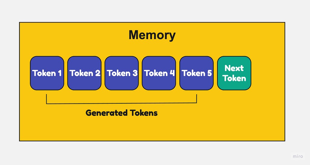
With paged attention, each page of keys/values can be placed anywhere in memory, non-contiguous. So if you free up some pages in the middle, that space can now be reused for other sequences.

This prevents fragmentation and allows higher memory utilization. Pages can be allocated and freed dynamically as needed when generating the output sequence.

2. Efficient KV Caching

KV caches stand for “key-value caches” and are used to cache parts of large language models (LLMs) to improve inference speed and reduce memory usage.

LLMs have billions of parameters, making them slow and memory- intensive to run inferences on. KV caches help address this by caching the layer outputs and activations of the LLM so they don’t need to be recomputed for every inference.

Here’s how it works:

• During inference, as the LLM executes each layer, the outputs are cached to a key-value store with a unique key.
• When subsequent inferences use the same layer inputs, instead of recomputing the layer, the cached outputs are retrieved using the key.
• This avoids redundant computations and reduces activation memory, improving inference speed and memory efficiency.

Alright, enough with the theory. Let’s deploy a model for real!

Hands-On Python Tutorial

There are two steps to deploy a model using TensorRT-LLM:

1. Compile the model
2. Deploy the compiled model as a REST API endpoint

Step 1: Compiling the model

For this tutorial, we will be working with Mistral 7B Instruct v0.2. As mentioned earlier, the compilation phase requires a GPU. I found the easiest way to compile a model is on a Google Colab notebook.

Google Colaboratory

TensorRT LLM is primarily supported on high end Nvidia GPUs. I ran the google colab on an A100 40GB GPU and will use the same GPU for deployment as well.

!git clone https://github.com/NVIDIA/TensorRT-LLM.git
%cd TensorRT-LLM/examples/llama

• Clone the TensorRT-LLM git repo. This repo contains all of the modules and scripts we need to compile the model.

!pip install tensorrt_llm -U --pre --extra-index-url https://pypi.nvidia.com
!pip install huggingface_hub pynvml mpi4py
!pip install -r requirements.txt

• Install the necessary Python dependencies.

from huggingface_hub import snapshot_download
from google.colab import userdata


snapshot_download(
    "mistralai/Mistral-7B-Instruct-v0.2",
    local_dir="tmp/hf_models/mistral-7b-instruct-v0.2",
    max_workers=4
)

• Download the Mistral 7B Instruct v0.2 model weights from hugging face and store them in a local directory at tmp/hf_models/mistral-7b-instruct-v0.2
• If you look inside the tmp/hf_models directory in Colab you should see the model weights there.

!python convert_checkpoint.py --model_dir ./tmp/hf_models/mistral-7b-instruct-v0.2 
                             --output_dir ./tmp/trt_engines/1-gpu/ 
                             --dtype float16

• The raw model weights cannot be compiled. Instead, they have to get converted into a specific tensorRT LLM format.
• The convert_checkpoint.py script takes the raw Mistral weights and converts them into a compatible format.
• The –model_dir is the path to the raw model weights.
• The –output_dir is the path to the converted weights.

!trtllm-build --checkpoint_dir ./tmp/trt_engines/1-gpu/ 
            --output_dir ./tmp/trt_engines/compiled-model/ 
            --gpt_attention_plugin float16 
            --gemm_plugin float16 
            --max_input_len 32256

• The trtllm-build command compiles the model. At this stage, you can pass in various optimization flags as well. To keep things simple, I have not used any additional optimizations.
• The –checkpoint_dir is the path to the converted model weights.
• The –output_dir is where the compiled model gets saved.
• Mistral 7B Instruct v0.2 supports a 32K context length. I’ve set that context length using the–max_input_length flag.

Note: Compiling the model can take 15–30 minutes

Once the model is compiled, you can upload your compiled model to hugging face hub. In order the upload files to hugging face hub you will need a valid access token that has WRITE access.

import os
from huggingface_hub import HfApi

for root, dirs, files in os.walk(f"tmp/trt_engines/compiled-model", topdown=False):
    for name in files:
        filepath = os.path.join(root, name)
        filename = "/".join(filepath.split("/")[-2:])
        print("uploading file: ", filename)
        api = HfApi(token=userdata.get('HF_WRITE_TOKEN'))
        api.upload_file(
            path_or_fileobj=filepath,
            path_in_repo=filename,
            repo_id="<your-repo-id>/mistral-7b-v0.2-trtllm"
        )

• This code uploads the compiled model, the .engine file, to hugging face under your user id.
• Replace the <your-repo-id> in the code with your hugging face repo which is usually your hugging face user id.

Awesome! That finishes the model compilation part. Onto the deployment step.

Step 2: Deploying the compiled model

There are a lot of ways to deploy this compiled model. You can use a simple tool like FastAPI or something more complex like the triton inference server.

When using a tool like FastAPI, the developer has to set up the API server, write the Dockerfile, and configure CUDA correctly. Managing these things can be a real pain and it ruins the overall developer experience.

To avoid these issues, I’ve decided to use a simple open-source tool called Truss. Truss allows developers to easily package their models with GPU support and run them on any cloud environment. It has a ton of great features that make containerizing models a breeze:

• GPU support out of the box. No need to deal with CUDA.
• Automatic Dockerfile creation. No need to write it yourself.
• Production ready API server
• Simple python interface

The main benefit of using Truss is that you can easily containerize a model with GPU support and deploy it to any cloud environment.

Creating the Truss

Create or open a python virtual environment with python version ≥ 3.8 and install the following dependency:

pip install --upgrade truss

(Optional) If you want to create your Truss project from scratch you can run the command:

truss init mistral-7b-tensort-llm

You will be prompted to give your model a name. Any name such as Mistral 7B Tensort LLM will do. Running the command above auto generates the required files to deploy a Truss.

To speed the process up a bit, I have a Github repository that contains the required files. Please clone the Github repository below:

GitHub – htrivedi99/mistral-7b-tensorrt-llm-truss

This is what the directory structure should look like for mistral-7b-tensorrt-llm-truss :

├── mistral-7b-tensorrt-llm-truss
│   ├── config.yaml
│   ├── model
│   │   ├── __init__.py
│   │   └── model.py
|   |   └── utils.py
|   ├── requirements.txt

Here’s a quick breakdown of what the files above are used for:

1. The config.yaml is used to set various configurations for your model, including its resources, dependencies, environmental variables, and more. This is where we can specify the model name, which Python dependencies to install, as well as which system packages to install.

2. The model/model.py is the heart of Truss. It contains the Python code that will get executed on the Truss server. In the model.py there are two main methods: load() and predict() .

• The load method is where we’ll download the compiled model from hugging face and initialize the TensorRT LLM engine.
• The predict method receives HTTP requests and calls the model.

3. The model/utils.py contains some helper functions for the model.py file. I did not write the utils.py file myself, I took it directly from the TensorRT LLM repository.

4. The requirements.txt contains the necessary Python dependencies to run our compiled model.

Deeper Code Explanation:

The model.py contains the main code that gets executed, so let’s dig a bit deeper into that file. Let’s first take a look at the load function.

import subprocess
subprocess.run(["pip", "install", "tensorrt_llm", "-U", "--pre", "--extra-index-url", "https://pypi.nvidia.com"])

import torch
from model.utils import (DEFAULT_HF_MODEL_DIRS, DEFAULT_PROMPT_TEMPLATES,
                   load_tokenizer, read_model_name, throttle_generator)

import tensorrt_llm
import tensorrt_llm.profiler
from tensorrt_llm.runtime import ModelRunnerCpp, ModelRunner
from huggingface_hub import snapshot_download

STOP_WORDS_LIST = None
BAD_WORDS_LIST = None
PROMPT_TEMPLATE = None

class Model:
    def __init__(self, **kwargs):
        self.model = None
        self.tokenizer = None
        self.pad_id = None
        self.end_id = None
        self.runtime_rank = None
        self._data_dir = kwargs["data_dir"]

    def load(self):
        snapshot_download(
            "htrivedi99/mistral-7b-v0.2-trtllm",
            local_dir=self._data_dir,
            max_workers=4,
        )

        self.runtime_rank = tensorrt_llm.mpi_rank()

        model_name, model_version = read_model_name(f"{self._data_dir}/compiled-model")
        tokenizer_dir = "mistralai/Mistral-7B-Instruct-v0.2"

        self.tokenizer, self.pad_id, self.end_id = load_tokenizer(
            tokenizer_dir=tokenizer_dir,
            vocab_file=None,
            model_name=model_name,
            model_version=model_version,
            tokenizer_type="llama",
        )


        runner_cls = ModelRunner
        runner_kwargs = dict(engine_dir=f"{self._data_dir}/compiled-model",
                             lora_dir=None,
                             rank=self.runtime_rank,
                             debug_mode=False,
                             lora_ckpt_source="hf",
                            )

        self.model = runner_cls.from_dir(**runner_kwargs)

What’s happening here:

• At the top of the file we import the necessary modules, specifically tensorrt_llm
• Next, inside the load function, we download the compiled model using the snapshot_download function. My compiled model is at the following repo id: htrivedi99/mistral-7b-v0.2-trtllm . If you uploaded your compiled model elsewhere, update this value accordingly.
• Then, we download the tokenizer for the model using the load_tokenizer function that comes with model/utils.py .
• Finally, we use TensorRT LLM to load our compiled model using the ModelRunner class.

Cool, let’s take a look at the predict function as well.

def predict(self, request: dict):

        prompt = request.pop("prompt")
        max_new_tokens = request.pop("max_new_tokens", 2048)
        temperature = request.pop("temperature", 0.9)
        top_k = request.pop("top_k",1)
        top_p = request.pop("top_p", 0)
        streaming = request.pop("streaming", False)
        streaming_interval = request.pop("streaming_interval", 3)

        batch_input_ids = self.parse_input(tokenizer=self.tokenizer,
                                      input_text=[prompt],
                                      prompt_template=None,
                                      input_file=None,
                                      add_special_tokens=None,
                                      max_input_length=1028,
                                      pad_id=self.pad_id,
                                      )
        input_lengths = [x.size(0) for x in batch_input_ids]

        outputs = self.model.generate(
            batch_input_ids,
            max_new_tokens=max_new_tokens,
            max_attention_window_size=None,
            sink_token_length=None,
            end_id=self.end_id,
            pad_id=self.pad_id,
            temperature=temperature,
            top_k=top_k,
            top_p=top_p,
            num_beams=1,
            length_penalty=1,
            repetition_penalty=1,
            presence_penalty=0,
            frequency_penalty=0,
            stop_words_list=STOP_WORDS_LIST,
            bad_words_list=BAD_WORDS_LIST,
            lora_uids=None,
            streaming=streaming,
            output_sequence_lengths=True,
            return_dict=True)

        if streaming:
            streamer = throttle_generator(outputs, streaming_interval)

            def generator():
                total_output = ""
                for curr_outputs in streamer:
                    if self.runtime_rank == 0:
                        output_ids = curr_outputs['output_ids']
                        sequence_lengths = curr_outputs['sequence_lengths']
                        batch_size, num_beams, _ = output_ids.size()
                        for batch_idx in range(batch_size):
                            for beam in range(num_beams):
                                output_begin = input_lengths[batch_idx]
                                output_end = sequence_lengths[batch_idx][beam]
                                outputs = output_ids[batch_idx][beam][
                                          output_begin:output_end].tolist()
                                output_text = self.tokenizer.decode(outputs)

                                current_length = len(total_output)
                                total_output = output_text
                                yield total_output[current_length:]
            return generator()
        else:
            if self.runtime_rank == 0:
                output_ids = outputs['output_ids']
                sequence_lengths = outputs['sequence_lengths']
                batch_size, num_beams, _ = output_ids.size()
                for batch_idx in range(batch_size):
                    for beam in range(num_beams):
                        output_begin = input_lengths[batch_idx]
                        output_end = sequence_lengths[batch_idx][beam]
                        outputs = output_ids[batch_idx][beam][
                                  output_begin:output_end].tolist()
                        output_text = self.tokenizer.decode(outputs)
                        return {"output": output_text}

What’s happening here:

• The predict function accepts a few model inputs such as the prompt , max_new_tokens , temperature , etc. We extract all of these values at the top of the function using the request.pop method.
• Next, we format the prompt into the required format for TensorRT LLM using the self.parse_input helper function.
• Then, we call our LLM model to generate the outputs using the self.model.generate function. The generate function accepts a variety of arguments that help control the output of the LLM.
• I’ve also added some code to enable streaming by producing a generator object. If streaming is disabled, the tokenizer simply decodes the output of the LLM and returns it as a JSON object.

Awesome! That covers the coding portion. Let’s containerize it.

Containerizing the model:

In order to run our model in the cloud we need to containerize it. Truss will take care of creating the Dockerfile and packaging everything for us, so we don’t have to do much.

Outside of the mistral-7b-tensorrt-llm-truss directory create a file called main.py . Paste the following code inside it:

import truss
from pathlib import Path

tr = truss.load("./mistral-7b-tensorrt-llm-truss")
command = tr.docker_build_setup(build_dir=Path("./mistral-7b-tensorrt-llm-truss"))
print(command)

Run the main.py file and look inside the mistral-7b-tensorrt-llm-truss directory. You should see a bunch of files get auto-generated. We don’t need to worry about what these files mean, it’s just Truss doing its magic.

Next, let’s build our container using docker. Run the commands below sequentially:

docker build mistral-7b-tensorrt-llm-truss -t mistral-7b-tensorrt-llm-truss:latest
docker tag mistral-7b-tensorrt-llm-truss <docker_user_id>/mistral-7b-tensorrt-llm-truss
docker push <docker_user_id>/mistral-7b-tensorrt-llm-truss

Sweet! We’re ready to deploy the model in the cloud!

Deploying the model in GKE

For this section, we’ll be deploying the model on Google Kubernetes Engine. If you recall, during the model compilation step we ran the Google Colab on an A100 40GB GPU. For TensorRT LLM to work, we need to deploy the model on the exact same GPU for inference.

I won’t go super deep into how to set up a GKE cluster as it’s not in the scope of this article. But, I will provide the specs I used for the cluster. Here are the specs:

• 1 node, standard kubernetes cluster (not autopilot)
• 1.28.5 gke kubernetes version
• 1 Nvidia A100 40GB GPU
• a2-highgpu-1g machine (12 vCPU, 85 GB memory)
• Google managed GPU Driver installation (Otherwise we need to install Cuda driver manually)
• All of this will run on a spot instance

Once the cluster is configured, we can launch it and connect to it. After the cluster is active and you’ve successfully connected to it, create the following kubernetes deployment:

apiVersion: apps/v1
kind: Deployment
metadata:
  name: mistral-7b-v2-trt
  namespace: default
spec:
  replicas: 1
  selector:
    matchLabels:
      component: mistral-7b-v2-trt-layer
  template:
    metadata:
      labels:
        component: mistral-7b-v2-trt-layer
    spec:
      containers:
      - name: mistral-container
        image: htrivedi05/mistral-7b-v0.2-trt:latest
        ports:
          - containerPort: 8080
        resources:
          limits:
            nvidia.com/gpu: 1
      nodeSelector:
        cloud.google.com/gke-accelerator: nvidia-tesla-a100
---
apiVersion: v1
kind: Service
metadata:
  name: mistral-7b-v2-trt-service
  namespace: default
spec:
  type: ClusterIP
  selector:
    component: mistral-7b-v2-trt-layer
  ports:
  - port: 8080
    protocol: TCP
    targetPort: 8080

This is a standard kubernetes deployment that runs a container with the image htrivedi05/mistral-7b-v0.2-trt:latest . If you created your own image in the previous section, go ahead and use that. Feel free to use mine otherwise.

You can create the deployment by running the command:

kubectl create -f mistral-deployment.yaml

It takes a few minutes for the kubernetes pod to be provisioned. Once the pod is running, the load function we wrote earlier will get executed. You can check the logs of the pod by running the command:

kubectl logs <pod-name>

Once the model is loaded, you will see something like Completed model.load() execution in 449234 ms in the pod logs. To send a request to the model via HTTP we need to port-forward the service. You can use the command below to do that:

kubectl port-forward svc/mistral-7b-v2-trt-service 8080

Great! We can finally start sending requests to the model! Open up any Python script and run the following code:

import requests

data = {"prompt": "What is a mistral?"}
res = requests.post("http://127.0.0.1:8080/v1/models/model:predict", json=data)
res = res.json()
print(res)

You will see an output like the following:

{"output": "A Mistral is a strong, cold wind that originates in the Rhone Valley in France. It is named after the Mistral wind system, which is associated with the northern Mediterranean region. The Mistral is known for its consistency and strength, often blowing steadily for days at a time. It can reach speeds of up to 130 kilometers per hour (80 miles per hour), making it one of the strongest winds in Europe. The Mistral is also known for its clear, dry air and its role in shaping the landscape and climate of the Rhone Valley."}

The performance of TensorRT LLM can be visibly noticed when the tokens are streamed. Here’s an example of how to do that:

data = {"prompt": "What is mistral wind?", "streaming": True, "streaming_interval": 3}
res = requests.post("http://127.0.0.1:8080/v1/models/model:predict", json=data, stream=True)

for content in res.iter_content():
    print(content.decode("utf-8"), end="", flush=True)

This mistral model has a fairly large context window, so feel free to try it out with different prompts.

Performance Benchmarks

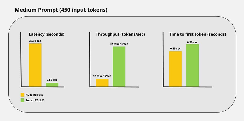
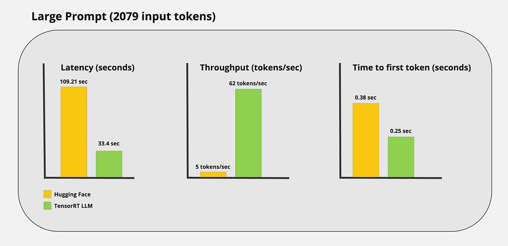
Just by looking at the tokens being streamed, you can probably tell TensorRT LLM is really fast. However, I wanted to get real numbers to capture the performance gains of using TensorRT LLM. I ran some custom benchmarks and got the following results:

Small Prompt:

Medium prompt:

Large prompt:

Conclusion

In this blog post, my goal was to demonstrate how state-of-the-art inference can be achieved using TensorRT LLM. We covered everything from compiling an LLM to deploying the model in production.

While TensorRT LLM is more complex than other inferencing optimizers, the performance speaks for itself. This tool provides state-of-the-art LLM optimizations while being completely open-source and is designed for commercial use. This framework is still in the early stages and is under active development. The performance we see today will only improve in the coming years.

I hope you found something valuable in this article. Thanks for reading!

Enjoyed This Story?

Consider subscribing for free.

Get an email whenever Het Trivedi publishes.

Images

If not otherwise stated, all images are created by the author.

---

Deploying LLMs Into Production Using TensorRT LLM was originally published in Towards Data Science on Medium, where people are continuing the conversation by highlighting and responding to this story.

Building an Azure Container App : A Data Analytics App with Python Flask, Plotly Dash, and Docker

Deploying scalable data analytics web applications: harnessing Flask, Dash, and Azure container apps for enhanced flexibility

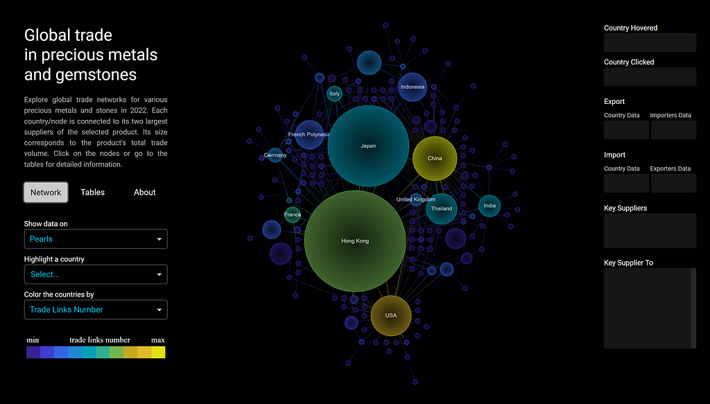
When it comes to developing data analytics web applications in Python, frameworks such as Plotly’s Dash and Streamlit are among the most popular today. But how do we deploy these frameworks for real applications, going beyond tutorials, while keeping scalability, efficiency, and cost in mind, and leveraging the latest cloud computing solutions?

In this article, we’ll cover the deployment of containerized applications using a Flask back-end with a Plotly Dash front-end, containerized with Docker, and deployed to Microsoft Azure’s Container App services. Instead of purely relying on the out-of-the-box Dash solution, we’ll deploy a custom Flask server. This approach adds flexibility to the application, enabling the use of Dash alongside other frameworks and overcoming some of the limitations of open-source Dash compared to Dash Enterprise.

Code sample for this tutorial is available on Github.

Microsoft Azure Container App Service

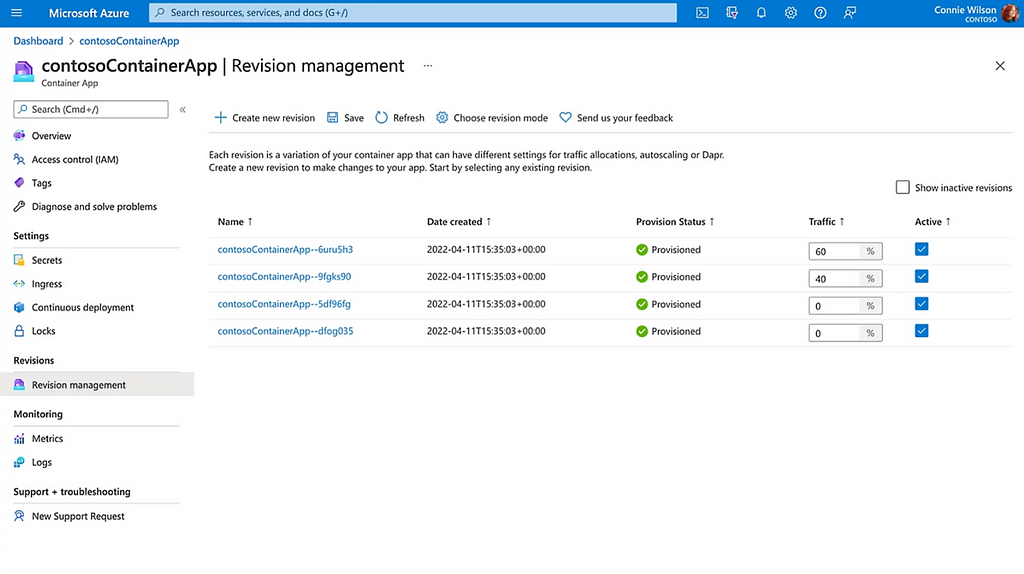
Azure Container Apps provide cost-effective, scalable, and fully managed app services utilizing a Kubernetes-based platform. A containerized application image, such as one created with Docker, can easily be deployed with a minimal amount of management required to run the application on the cloud. Most of the heavy lifting is managed by Azure, offering scalability at a manageable cost.

The scalable cost option is ideal for intranet-based applications where most of the consumption occurs internally, with users interacting with the application in a manner similar to how they would with PowerBI or Tableau services. However, unlike PowerBI or Tableau, hosting a data web application offers the advantage of not requiring user license costs, along with the flexibility to overcome limitations of these dashboarding tools. When combined with the ease of development in Python, powered by frameworks such as Plotly Dash, it presents a strong alternative to other dashboarding solutions.

Plotly Dash

Plotly is a popular data visualization framework, available in multiple programming languages such as Python, R, JavaScript, and Matlab. Dash, developed by Plotly, is a framework for building highly interactive data applications. It employs a Python Flask server and utilizes React for building interactive web applications, enabling users to develop data applications entirely in Python. Additionally, it offers the flexibility to integrate custom HTML/CSS/JavaScript elements as needed.

Although alternatives like Streamlit exist for building data analytics applications in Python, this article will specifically cover Dash due to its use of Python Flask for backend services. Dash’s utilization of Flask provides significant flexibility, allowing for various applications to coexist on the same website. For example, certain sections of an app could be built using pure HTML/CSS/JavaScript or React, while others might incorporate embedded PowerBI reports.

Dash is available in two flavors: open source and enterprise. We will focus on the open-source version, addressing its limitations such as security management, which can be enhanced through the use of a custom Flask server.

Flask

Python’s Flask library is a lightweight yet powerful web framework. Its lightweight design is particularly suited for data analytics professionals who may not have extensive web development experience and prefer to start with a minimalistic framework.

Flask also powers the backend server for Dash. When developers create a Dash application, a Flask server is automatically initiated. However, in this article, we’ll explore deploying a custom Flask server. This approach maximizes the flexibility of Flask, extending beyond the use of Dash in our application. It enables the entire web application to utilize other frameworks in addition to Dash and facilitates the construction of authentication pipelines. Such features are not included in the open-source version of Dash without this customization but are available in the Enterprise version.

Local App Development

Local Development Prerequisites

There are a few prerequisites for setting up the local development environment. While not all of them are strictly required, it is highly recommended to follow the guidelines provided below. It’s important to note that this tutorial was created using a Windows 11 machine. Some modifications may be necessary for other operating systems.

• Download Python. This tutorial uses Python 3.10.11. Its highly recommended to add Python to PATH during or after installation.
• Download Azure CLI. This will be used to connect to Azure locally via terminal.
• Download Docker.
• Download VS Code.
• VS Code Azure Extension.
• VS Code Azure Container Apps Extension.
• VS Code Docker Extension.

App Structure

Below is the outline of the demo app’s structure, designed to host multiple applications within the web application, all powered by a Flask server.

AZURE_DATA_ANALYTICS_WEBAPP/
|---|main.py
|---|figures.py
|---|assets/
|---|static/
|------|css/
|------|js/
|------|img/
|---|templates/
|------|home.html
|---|requirements.txt
|---|Dockerfile
|---|.dockerignore
|---|.gitignore
|---|.env
|---|.venv
|---|README.md

Python Local Environment Setup

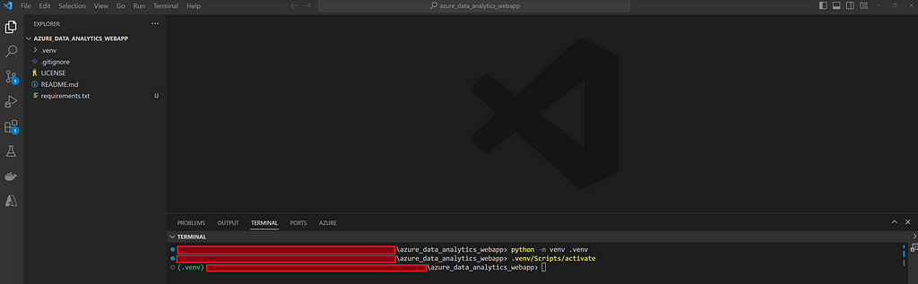
We’ll begin by creating a Python virtual environment named .venv in the VS Code terminal using the commands provided below. Be sure to include .venv in both the .gitignore and .dockerignore files, as these should not be uploaded or deployed.

python -m venv .venv
.venv/Scripts/activate
pip install --upgrade pip
pip install -r requirements.txt

The requirements for the project are listed in the requirements.txt file as follows:

# requirements.txt

# Web App Framework Requiremed Files:
Flask==3.0.2
plotly==5.19.0
dash==2.15.0
gunicorn==21.2.0

# Azure required files:
azure-identity==1.15.0
azure-keyvault-secrets==4.7.0

# Other Utilities:
python-dotenv==1.0.1
numpy==1.26.4
pandas==2.2.0

Flask Server

The main entry point to the application will be main.py, where we will initialize and run the application. In this file, we will define the Flask server, which will serve as the backend server for the entire application.

At this stage, we don’t have any Dash apps integrated; there’s just a single route defined at the index page of our application that renders the home.html file. A route is a URL pattern that handles and executes HTTP requests matching that pattern. In our case, we have a home route. Upon accessing the main directory of the web application (“/”), the home.html file will be rendered.

# main.py

from flask import Flask, render_template

# Initialize Flask server:
# Let Flask know where the templates folder is located
# via template_folder parameter
server = Flask(__name__, template_folder = "templates")

# Define Routes:
@server.route("/")
def home():
    """
        Index URL to render home.html
    """
    return render_template("home.html")

# Run the App:
if __name__ == "__main__":
    server.run(host = "0.0.0.0", port = 5000, debug = True)
    # Set debug to False during production

<!-- templates/home.html file -->

<!DOCTYPE html>
<html>
<head>
    <title>Azure Data Analytics Web Application</title>
</head>
<body>
    <h1>Azure Container App Data Analytics Application
     with Python Flask, Plotly Dash & Docker
    </h1>
</body>
</html>

Note that Flask expects HTML templates to be stored under the templatesfolder. Flask utilizes Jinja to parametrize the HTML templates.

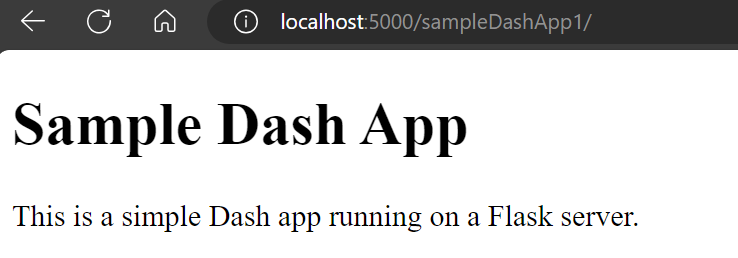
We are now ready to run our application locally for the first time. Please note that the debug mode is currently set to true, as shown above. Remember to set this to false for production deployment. To run the app locally, execute the command provided below and then visit http://localhost:5000/ in your browser.

python main.py

We should note that when running locally, as in the above example, the application does not use HTTPS. However, Azure Container App significantly simplifies development work by handling most of the heavy lifting related to SSL/TLS termination.

It’s also important to mention that the local execution of the application utilizes the default Flask HTTP server. For production deployment, however, we bind the application to a Gunicorn server while creating the Docker image. Gunicorn, a Python WSGI HTTP server for Unix, is better suited for production environments. The installation of Gunicorn is included in the requirements.txt file.

Dash App

Now, we will modify the main.py file to add an instance of a Dash app. In this step, we initialize the Dash app by providing the Flask server, specifying the base URL pathname for routing to the app, and indicating which assets folder to use. The assets folder can store images and custom style CSS files for the Dash app.

# main.py

from flask import Flask, render_template
from dash import Dash, html

# Initialize Flask server:
server = Flask(__name__, template_folder = "templates")

# Define Routes:
@server.route("/")
def home():
    """
        Redirecting to home page.
    """
    return render_template("home.html")

# Dash Apps:
app1 = Dash(__name__, server = server,
  url_base_pathname = "/sampleDashApp1/",
  assets_folder = "assets")

app1.layout = html.Div([
    html.H1("Sample Dash App"),
    html.P("This is a simple Dash app running on a Flask server.")
])

# Run the App:
if __name__ == "__main__":
    server.run(host = "0.0.0.0", port = 5000, debug = True)
    # Set debug to False during production

Dash supports most HTML tags, which can be specified directly in Python, as illustrated in the example above. So far, we’ve added H1 header and P paragraph tags. Furthermore, Dash allows the addition of other elements, such as Dash Core Components. This feature enables us to incorporate widgets as well as plots from the Plotly library.

Adding Plotly Figures

We will define some sample Plotly charts in the figures.py file and subsequently incorporate them into the Dash app.

# figures.py

import plotly.express as px
import pandas as pd
import numpy as np

def line_chart():
    """
        Sample Plotly Line Chart
    """
    df = pd.DataFrame({
        "X": np.linspace(0, 10, 100),
        "Y": np.sin(np.linspace(0, 10, 100))
    })

    fig = px.line(df, x = "X", y = "Y", title = "Line Chart")

    return fig

def bar_chart():
    """
        Sample Plotly Bar Chart
    """

    df = pd.DataFrame({
        "Category": ["A", "B", "C", "D", "E"],
        "Values": np.random.randint(10, 100, size = 5)
    })

    fig = px.bar(df, x = "Category", y = "Values", title = "Bar Chart")

    return fig

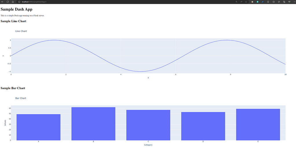
If we modify the main.py file to import bar_chart and line_chart from the figures.py file, we can then add these plots as graph elements to our Dash app, as shown below.

# main.py file

# ...Rest of the code

from figures import line_chart, bar_chart

# Dash Apps:
app1 = Dash(__name__, server = server,
  url_base_pathname = "/sampleDashApp1/",
  assets_folder = "assets")

app1.layout = html.Div([
    html.H1("Sample Dash App"),
    html.P("This is a simple Dash app running on a Flask server."),
    html.H2("Sample Line Chart"),
    dcc.Graph(figure=line_chart()),
    html.H2("Sample Bar Chart"),
    dcc.Graph(figure=bar_chart())
])

# ... Rest of the code

Building and Running Docker Image Locally

We have now established a skeleton code for our application and are ready to build our Docker image. First, we need to enable virtualization from the motherboard’s BIOS settings, which is essential for creating virtual machines that Docker relies on. Secondly, the Docker software and the VS Code Docker Extension need to be installed.

Once the above steps are completed, we create a Dockerfile in our main directory and enter the following:

# Dockerfile

# Set Python image to use:
FROM python:3.11-slim-bullseye

# Keeps Python from generating .pyc files in the container:
ENV PYTHONDONTWRITEBYTECODE=1
# Turns off buffering for easier container logging:
ENV PYTHONUNBUFFERED=1

# Install requirements:
RUN python -m pip install --upgrade pip
COPY requirements.txt .
RUN python -m pip install -r requirements.txt

# Set Working directory and copy files:
WORKDIR /app
COPY . /app

# Creates a non-root user with an explicit UID
# and adds permission to access the /app folder:
RUN adduser -u 5678 --disabled-password --gecos "" appuser && chown -R appuser /app
USER appuser

# Expose port 5000:
EXPOSE 5000

# Bind to use Gunicorn server
# and specify main entry point main.py/server object:
CMD ["gunicorn", "--bind", "0.0.0.0:5000", "main:server"]

To build the Docker image, we execute the following command in the terminal:

docker build --no-cache -t app:version1 .

With this step completed, we should see a Docker image created, visible in the VS Code Docker extension. In this instance, we have specified the name of the app as ‘app’ and the version of the image as ‘version1’.

Now we are ready to run the app locally. To create and start a local Docker container, we execute the following command in the terminal:

docker run --env-file ./.env -p 5000:5000 app:version1

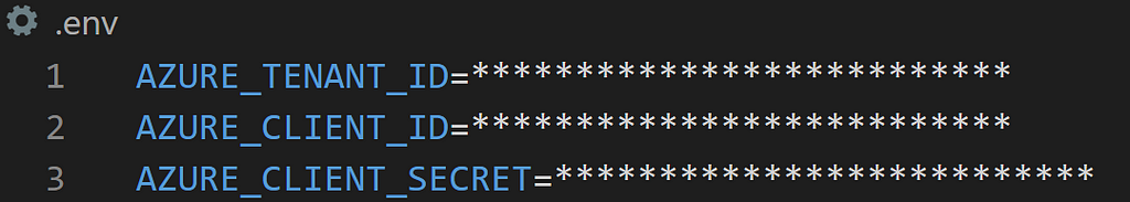
This will start the Docker container locally, allowing us to navigate to the app in the browser at http://localhost:5000/. In the Docker run command mentioned above, we instruct Docker to use the .env file located in the main directory as the environmental variables file. This file is where we store app configuration variables and any secrets. It’s crucial to note that the .env file must be included in both .gitignore and .dockerignore files, as we do not want sensitive information to be uploaded to Git or included in the Docker container. On Azure Container Apps, these parameters can be provided separately as environmental variables.

For our basic Azure deployment case, there is no need to provide any environmental variables at this stage.

Below is the content of the .dockerignore file:

**/__pycache__

**/.vscode
**/.venv
**/.env
**/.git
**/.gitignore

LICENSE
README.md

Azure Setup & Deployment

Now that we have a working application locally and have successfully created a Docker image, we are ready to set up Azure and deploy the Container App.

To proceed with the steps outlined below, it is necessary to have the Azure CLI (a terminal application for communicating with Azure) installed, along with the VS Code Azure Container Apps extension.

Setup Azure Subscription

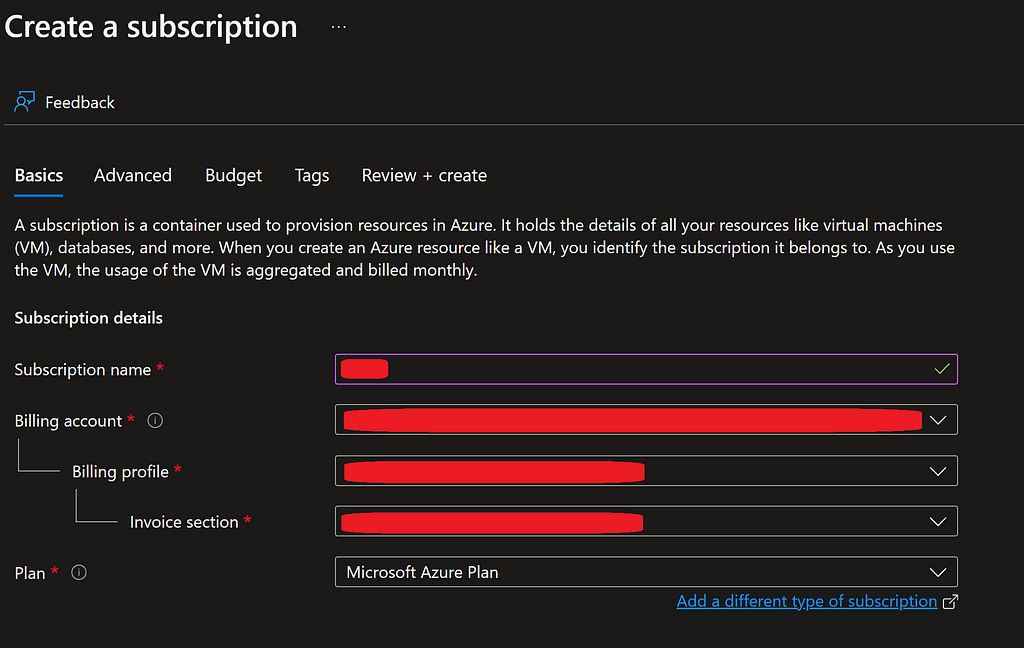
Once we have created an Azure account, the first step is to create a Subscription. A Subscription on Azure contains a collection of Azure resources linked to a billing account. For first-time Azure users or students, there are credits available ranging from $100 to $200. In this tutorial, however, we will focus on setting up a paid account.

After signing up and logging into Azure, we navigate to ‘Subscriptions’, which will be tied to our billing account. Here, we need to provide a name for the subscription and proceed with its creation.

Note: Special care should be taken to monitor billing, especially during the learning period. It’s advisable to set budgets and alerts to manage costs effectively.

Setup Azure Resource Group

Azure manages a collection of cloud resources under what is known as an Azure Resource Group. We’ll need to create one of these groups to facilitate the creation of the necessary cloud resources.

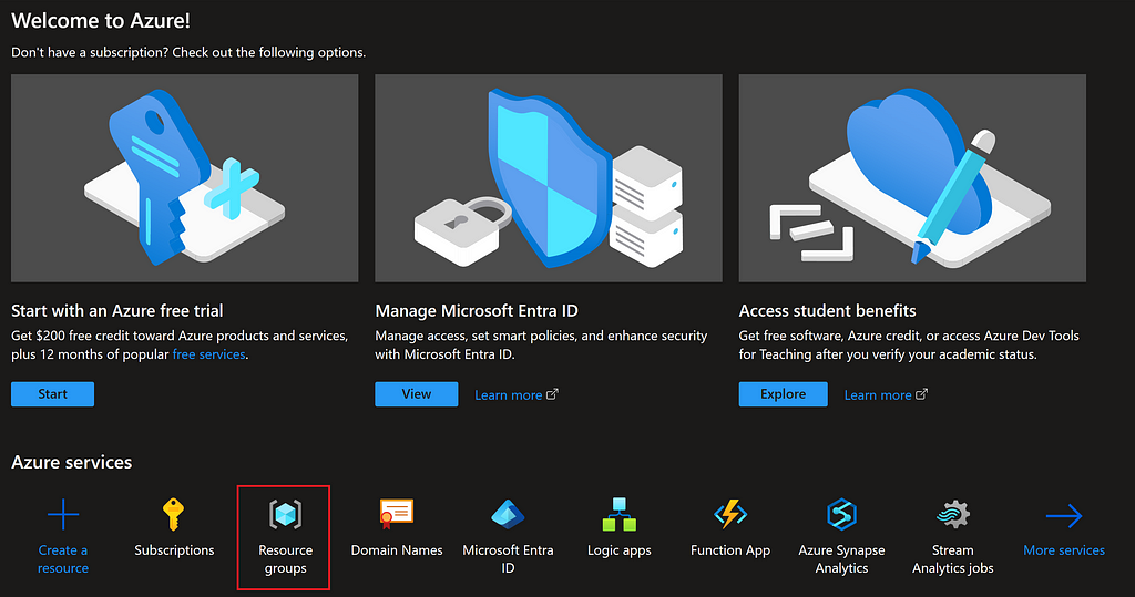
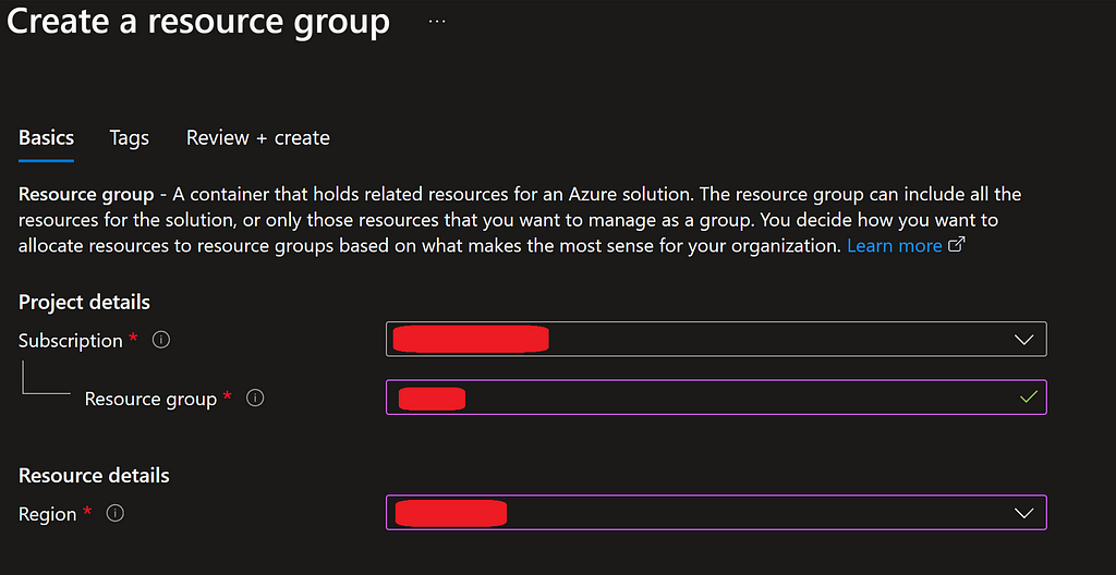
From the main Azure page, we can navigate to ‘Resource Groups’ to create a new one.

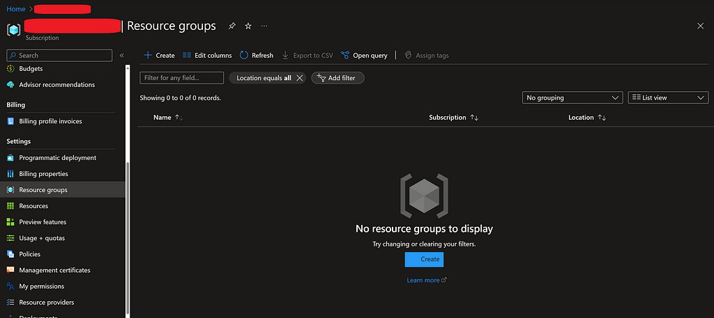
This Resource Group will be associated with the Subscription we created in the previous step. We will need to provide a name for the Resource Group and select a region. The region should be chosen based on the closest geographical area to where the application will be primarily used.

Setup Azure Container Registry

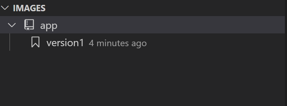
Azure offers a container registry service known as Azure Container Registry, which allows us to host our Docker container images. This container registry serves as a repository for images, enabling version control over the container images. It also facilitates their deployment across various cloud container services, not limited to Azure Container Apps alone. With this service, different versions of the app image can be stored and deployed as needed.

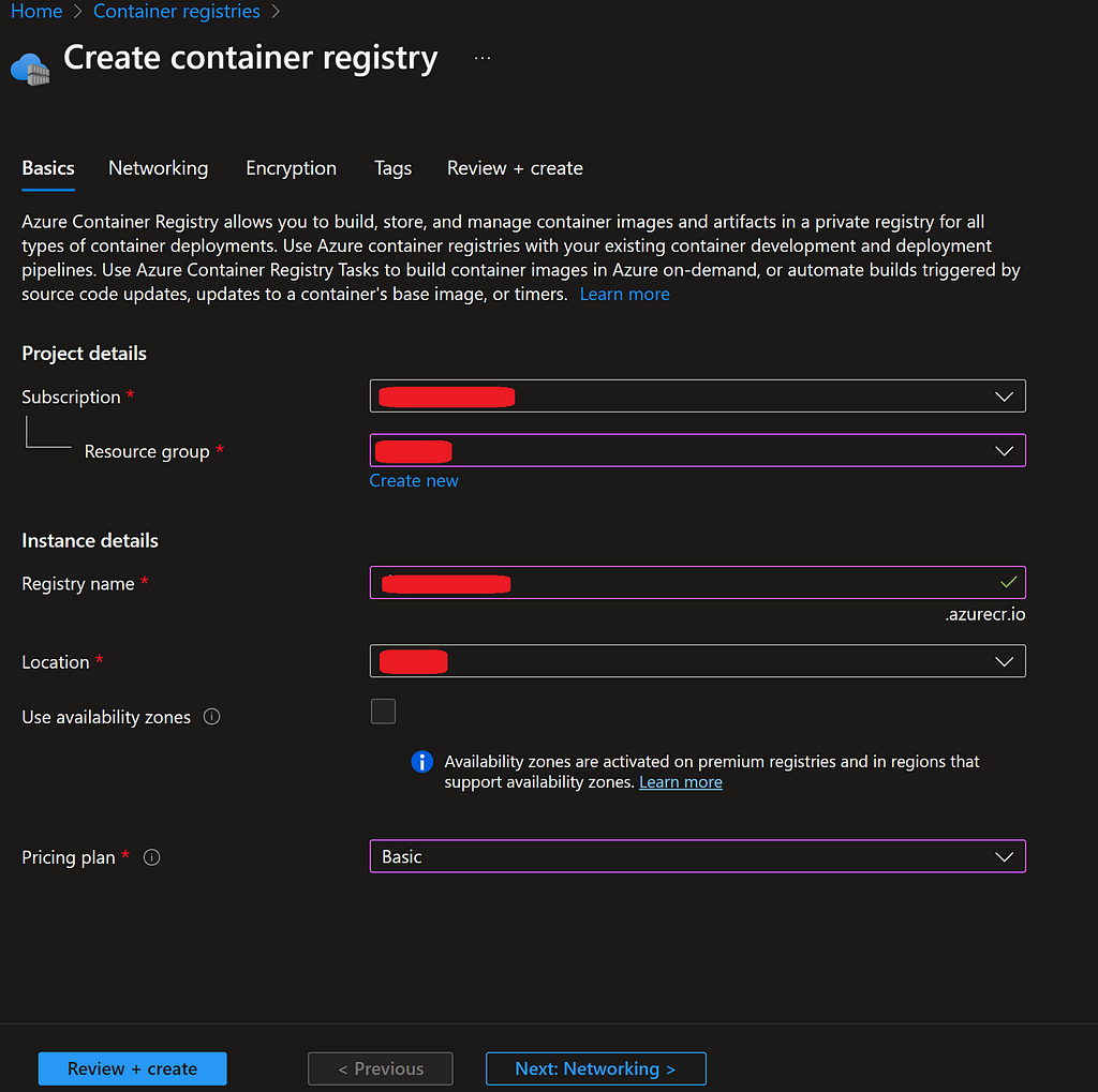
From the search bar in the Azure portal, we type ‘Container Registries’ and click the create button. This resource will be hosted under the Resource Group we created in the previous step. We should choose the same region as before and select the Basic plan option for the lowest cost.

There is one important setting that needs to be enabled on the Container Registry to allow us to deploy images to Azure Container App within the Azure portal. Go to the Properties of the Container Registry, enable the ‘Admin user’, and then save the changes.

Deploy Docker Image to Azure Container Registry

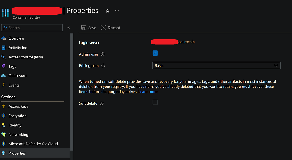
Now that we have our local Docker image ready and the Azure Container Registry setup complete, we are prepared to upload the container image to Azure.

In the VS Code terminal, we log in to Azure using the Azure CLI (which must be installed):

az login

This action will open a pop-up window in your browser, prompting you to sign in to Azure. Once completed, we are now authenticated with Azure.

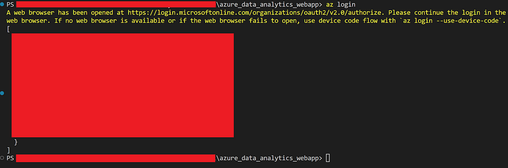
The next step is to log in to the Container Registry using the terminal and Azure CLI. This can be done by executing the following command:

az acr login --name <azureContainerRegistryName>

Once we have successfully logged in to the Container Registry, our next steps are to first tag the image and then push it to the Azure Container App.

Note that ‘app:version1’ represents the name and version of our app, which we assigned when creating the Docker image in the previous steps.

docker tag app:version1 <azureContainerRegistryName>.azurecr.io/app:version1
docker push <azureContainerRegistryName>.azurecr.io/app:version1

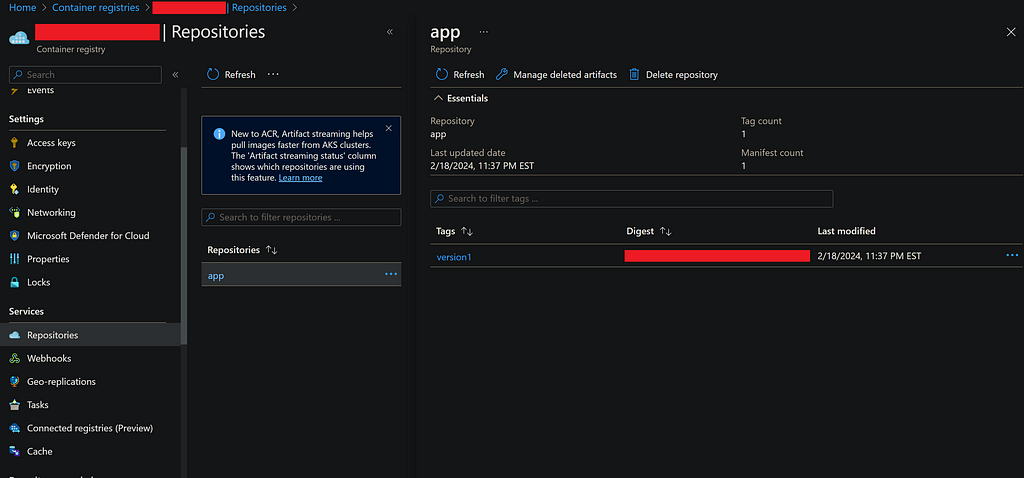
With this step completed, we should be able to view the image under the ‘Repositories’ section of the Container Registry, as described above.

It’s important to note that the above steps could also have been accomplished using the VS Code Docker Extension, as an alternative to utilizing the Azure CLI.

Setup Azure Container Apps Environment & Container App

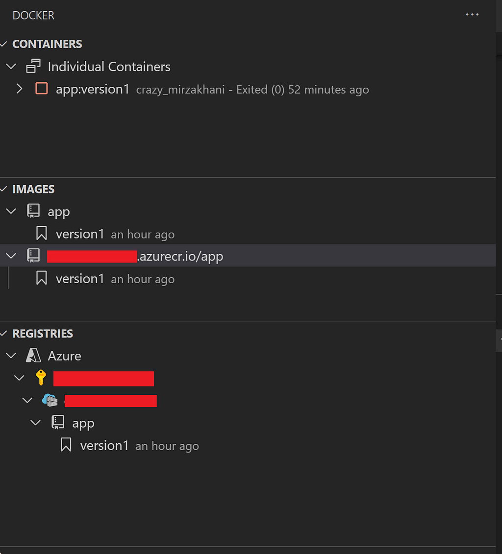
The Azure Container Apps Environment is a resource that can manage a collection of container apps. While we cannot create a Container Apps Environment directly, it can be set up when we create an initial Container App.

To do this, we search for ‘Container Apps’ in the Azure search bar and click ‘Create’. The first step here is to create a Container Apps Environment, as highlighted in the red square box in the image below.

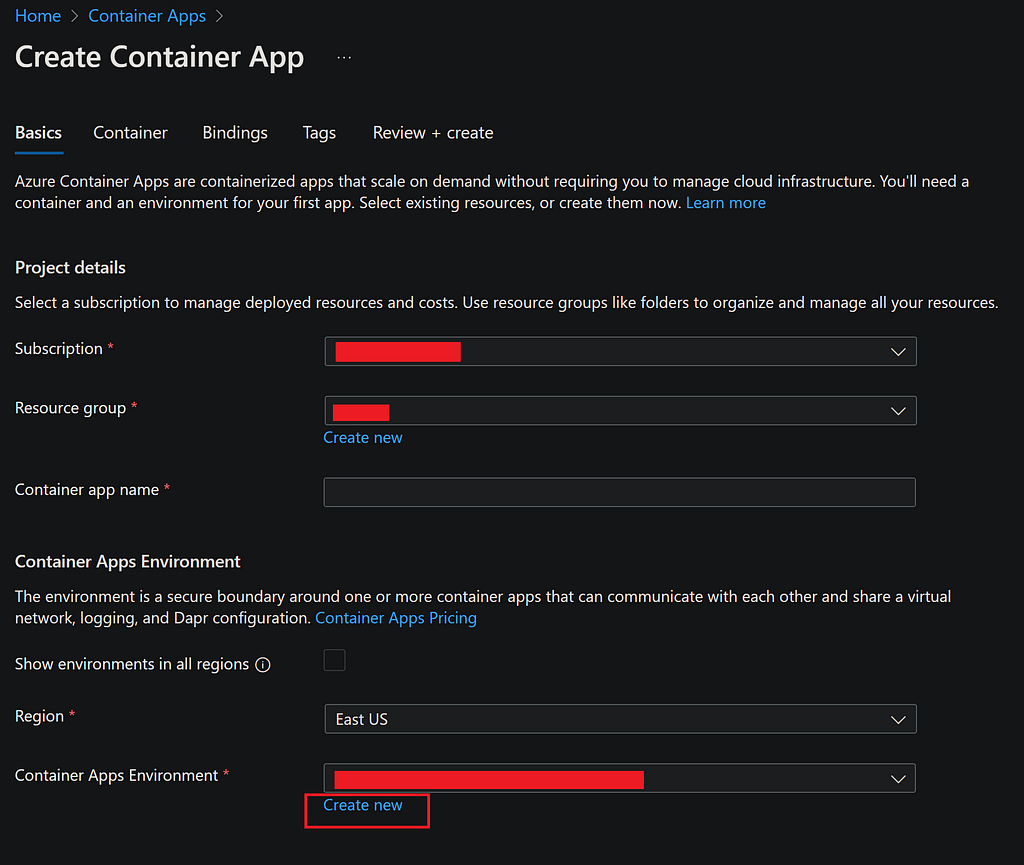
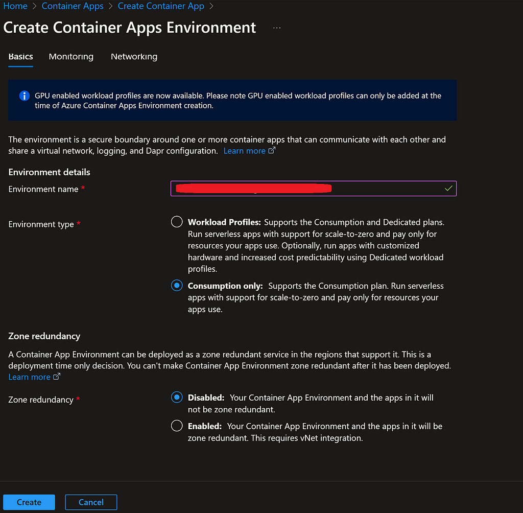
We select the consumption plan to pay only for what we use and for providing a simplified setup process.

After creating the Container Apps Environment, we return to the setup page for the Container App to continue building the app. Within the Container setup page, we select Azure Container Registry and locate the image we have previously uploaded.

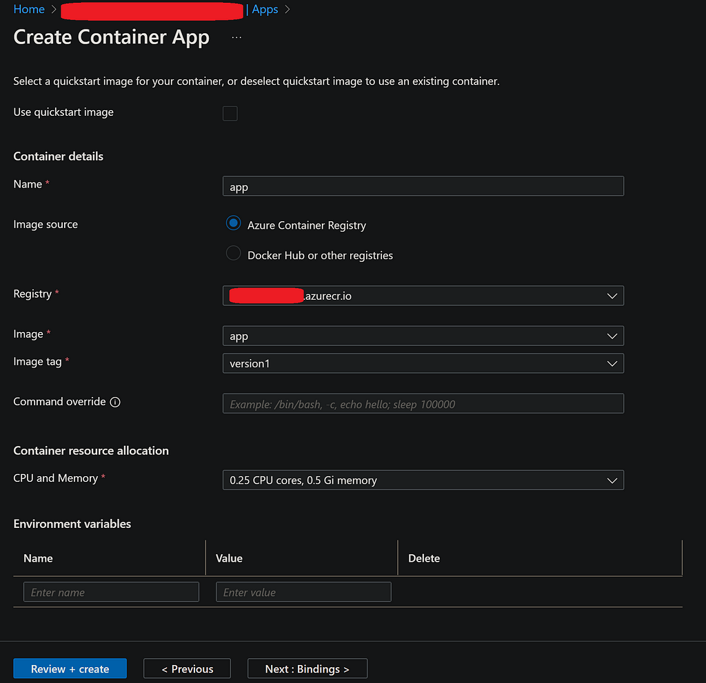
For CPU and memory, we opt for the lowest amount as this is a demo app. If there are any environmental variables specified in the .env file for our local environment, we must enter them in this section. Alternatively, these environmental variables can be directed to Azure KeyVault.

We can skip the Bindings section for this tutorial and proceed to Ingress. In this section, we define how Azure Container App handles traffic. We enable Ingress and set traffic to be accepted from anywhere if the application is to be accessible on the web. For internal applications, the company’s VNet should be used.

Additionally, we set the port of the application to be 5000, which is the same as the Flask server’s port set during code development.

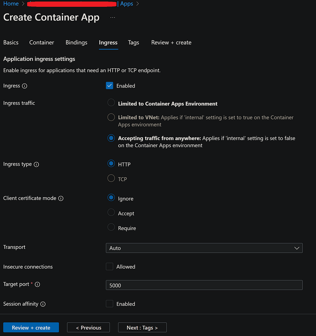
After configuring all of these settings, we are ready to create our application! Click on ‘Review + create’.

Once the setup is complete, navigate to the Container App page to find the URL of the application.

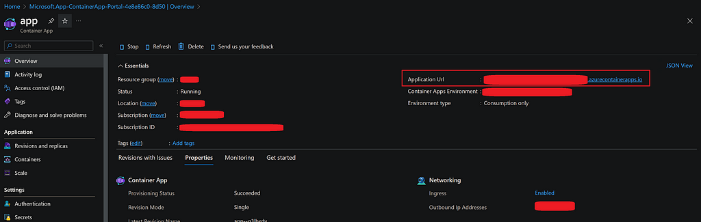
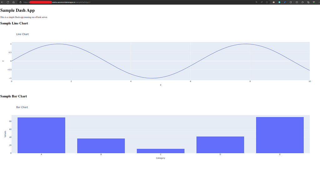
And that’s it! Our application is now up and running on Azure!

Manage Revisions

Now that we have deployed the first version of our application, we’ll cover managing revisions.

Once we have made changes to the code base and ready with a revision, we run Docker deploy as before with a new version name.

docker build --no-cache -t app:version2 .

And upload to Azure Container Registry:

az acr login --name <azureContainerRegistryName>
docker tag app:version2 <azureContainerRegistryName>.azurecr.io/app:version2
docker push <azureContainerRegistryName>.azurecr.io/app:version2

From here on, we have two options. Either to use terminal and Azure CLI or go to Azure Container App page and manage revisions from there. Here we will cover revision management from Azure.

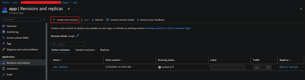
Hit “Create new revision” and provide a suffix to the new revision. Here we’ll name it “version2”. Than click on “app” check-box and select edit.

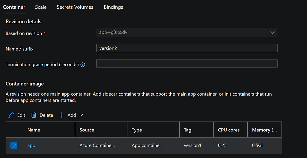
In edit container section, select the new version of the image from Azure Container Registry and save. Once complete, press create and new revision will be created.

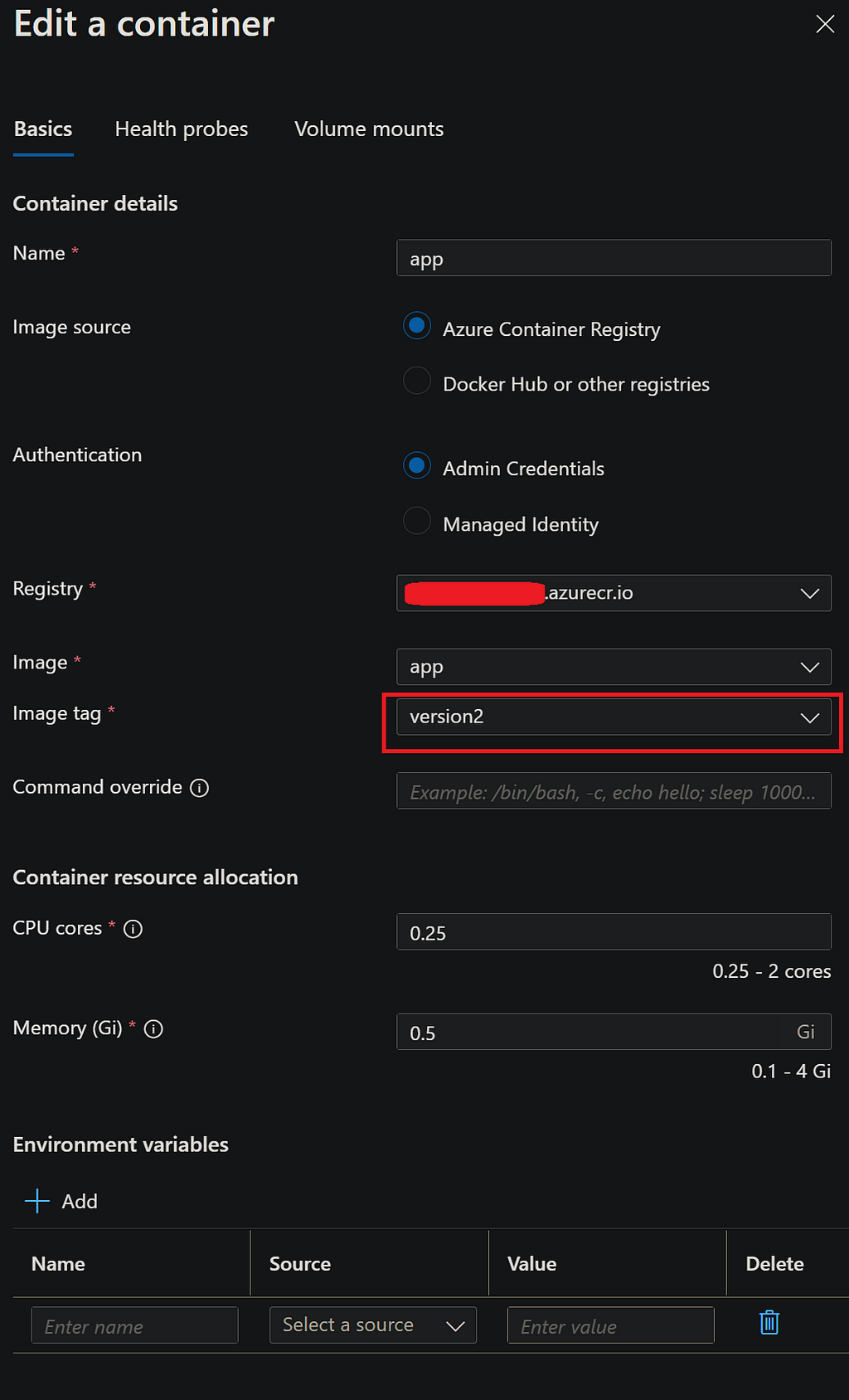
When we come back to Revisions, we see the new container revision is taking 100% of the traffic. Although the old revision still remains and can be de-activated via Azure CLI.

Further Considerations

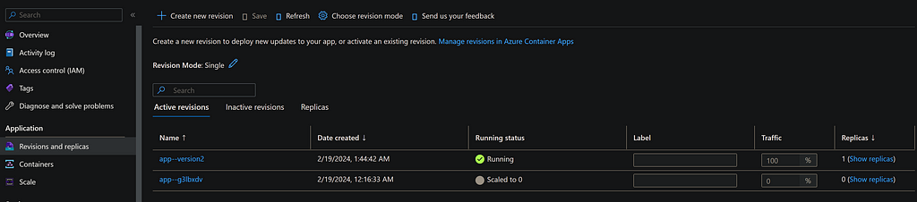
We have successfully deployed a Container App to Azure using Python Flask & Dash. However, this application is far from ready for production release.

For internal applications, an authentication process needs to be considered. Using Azure Active Directory and the Python MSAL library, it is possible to define roles and access lists for users within a company’s directory and control the authentication flow with a Flask server. The Dash Enterprise version enables this integration in a much easier way. However, the Enterprise version might not be an option for everyone. We must remind again that the choice of using a custom Flask server in our Dash application was made to overcome the lack of authentication support in the open-source version. Adding Microsoft Active Directory authentication pipeline will be covered in a future article.

At this stage, the app is only using some demo plots and synthetic data. With the app being deployed on Azure, we have many options to serve our data to the app. The first option is to utilize Azure Data Lake Storage for a cost-effective file-based storage solution. While this option provides storage at a very low cost, it puts the burden of computation on the web app. Another alternative is to utilize Azure Databricks and its SQL Endpoint to offload heavy data computations to a cloud cluster. These topics will be covered again in another tutorial.

References

1. Overview of Python Container Apps in Azure — Python on Azure | Microsoft Learn

---

Azure Container App, a Data Analytics WebApp with Python Flask, Plotly Dash & Docker was originally published in Towards Data Science on Medium, where people are continuing the conversation by highlighting and responding to this story.

Implementing in real life the different frameworks we’ve seen

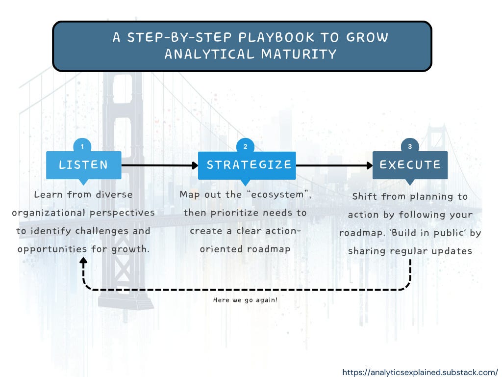
.. And we’re back on our articles on Analytical Maturity! One of the feedback that I received on the previous installments was that those articles might be too high level and it would be great to have something slightly more actionable. So that’s what we’re going to do today: make the whole thing more actionable via a step-by-step on how to grow an organization’s analytical maturity.

Let’s start with step #1: Shutting up and listening!

Step #1: Shut up and listen

There is this great TED video by Ernesto Sirolli called “Want to help someone? Shut up and Listen”. In it, he explained how, as a 21 years-old, he worked for an Italian NGO which tried to “teach Zambian people how to grow food”. They successfully grew magnificent tomatoes in the valley down by the Zambezi river — but, as Sirolli puts in his own words:

When the tomatoes were nice and ripe and red, overnight, some 200 hippos came out from the river and they ate everything. And we said to the Zambians, ‘My God, the hippos!’ And the Zambians said, ‘Yes, that’s why we have no agriculture here.’

Whenever you want to grow your organization’s analytical maturity, the first step is going to shut up and just listen. You need to listen and understand the pain points, the different jobs, the data needs, what has been done in the past to solve those pain points, etc. Not only will this give you a better perspective of the lay of the land, it will also give you a better understanding of the people that are part of your organization.

“Listening” In the context of a medium or large organization means actively gathering information. To do so, you have a couple of efforts that you can run:

• User Interviews: Deep dive into the individual experiences of your team members to gather qualitative insights into their daily challenges, data usage, and specific pain points. By engaging directly and in a small setting, you create an open channel for honest feedback and nuanced understanding of the data needs across your organization.
• Running Surveys: Surveys (especially anonymous ones) give you the ability to collect a broader range of insights from a larger segment of your organization. This not only helps in identifying common themes and areas of concern but also serves as a tool for establishing benchmarks for satisfaction and data literacy levels within your organization.
• Joining Team Meetings: Participating in regular team meetings across different departments allows you to observe firsthand how data is currently being used in decision-making processes, identify gaps in data availability or accessibility, and note the common questions or misconceptions that arise when data is discussed.
• Shadowing People’s Jobs: Try immersing yourself in the lives of your users. This will provide you with a raw look at the operational challenges faced by teams and individuals, offering invaluable insights into how analytical tools and data are integrated (or not) into everyday workflows.

Using those different methods, you can do a lot of great listening that will give you a comprehensive understanding of where your organization stands in terms of analytical maturity and where the most impactful improvements can be made. This is a very foundational stage — part of the diagnosis phase, that will help you shape your strategy.

Now should you listen to everything everywhere all at once? If you don’t want to end up like Jobu Tupaki — it is important to make sure to adopt the right lens during your exploration.

• In terms of depth, some problems will require you to use a microscope (because they are very technical, very complex, and very sensitive) while some will be better observed from afar (because they are low priority and don’t necessarily require your involvement). I don’t have any ready-made framework for that here, but part of your diagnosis phase is about getting this understanding.
• In terms of width, using the framework “Tools / Processes / People / Culture” is usually a good starting point. You want to have a good understanding of the people of your org, their skillset, and what motivates them; you want to understand their processes and how they work together and with the other stakeholders; and you want to be clear on the tool they use.

Step #2a: Prioritize, build a roadmap and communicate

Once you have a good understanding of the different organizational pain points, and why they exist, you can start preparing a strategy. As I mentioned in a previous article — following Richard Rumelt’s framework, a good strategy is made of 3 elements: a diagnosis, a guiding policy, and an action plan.

At this stage, thanks to all your listening from the previous section, you should feel well-equipped to start documenting needs and start pinpointing where the gaps are in your current organization. Hopefully at this point creating the following “mappings” shouldn’t be an issue:

• Skill set mapping (who inside the team can do what)
• Activity / Project mapping (who inside the team is doing what)
• Process mapping (how we decide what to do and how it is being done)
• Tools mapping (what tools do we use to do what we want to do)
• Stakeholder mapping (who outside of the team cares about / can influence what we do)
• Goal mapping (what are the top goals of the different teams and how they relate to each other)
• Etc.

From experience, as you put together those different maps, you will start encountering interesting insights about your team and your organization, and more generally you will start understanding how the whole “system” works together. It is usually after this stage that you realize that some tools are being used because some skillsets are not available, some processes exist as a workaround around faulty tools, etc. Basically this is at this step that you’ll find out about the little inefficiencies. And so hopefully after this long mapping exercise, you should see a few areas for improvement — and this is where you need to move from exploration to action:

• Adopt a Prioritization Process: Establish a clear and transparent method for prioritizing the needs you just documented. This could involve criteria such as impact on business goals, frequency of the issue, or the ease of implementation. Consider frameworks like MoSCoW (Must have, Should have, Could have, Won’t have this time) or ICE scores (Impact, Confidence, Ease) to methodically assess each need.
• Prioritize Accordingly: Use your chosen prioritization process to rank the needs from most critical to least. This step ensures that resources are allocated effectively to areas with the highest potential for impact on the organization’s analytical maturity.
• Create and Share Your Roadmap: Adopt a clean roadmap, with clear deliverables and a clear timeline. Communication is key in setting expectations and building support for your initiatives. Share the prioritized list and the rationale behind the ranking with your stakeholders. This transparency helps in managing expectations, securing buy-in, and fostering a collaborative approach to improving the organization’s data capabilities.

By following these steps, you create a focused and strategic roadmap that addresses the most pressing data needs within your organization. This roadmap not only sets clear expectations but also aligns your data initiatives with the overall business objectives, ensuring a cohesive and effective approach to enhancing analytical maturity.

Note that while the diagnosis gave you the areas for improvement, sometimes it is not necessarily clear what the solution should be. There are two frameworks that I like to use in those kind of situations:

• Action > Information > Vision: A lot of the time, your vision will come from additional information that will come from you taking action. You do something and learn from it, and this helps you shape your vision. So if you are not sure where to go, take the first very little step you can — from there you’ll be at a different venture point, and most likely the next steps will appear.
• Innovation > Quantification > Orchestration: This framework that comes from “The E-Myth Revisited: Why Most Small Businesses Don’t Work and What to Do About It” by Michael E. Gerber is great for when you try to optimize a process: just select a piece of the process, “innovate” (i.e. change it), quantify this innovation (is the process better with this change?) and if the quantification is positive, orchestrate (i.e. remove the human decision making component out of it).

So if you are not sure about what the solution should be and what the deliverable in your roadmap should be — either break your problem down and focus on the very next step, or run a pilot for a potential solution.

Step #2b: Get some quick wins to build credibility

This step — while optional, is generally recommended. If you need to build some credibility, you might want to prioritize some quick wins, as this will allow you to build trust and put you and your team on a “momentum” of deliveries.

• Identify Low-Hanging Fruit: Look for projects or improvements that can be implemented quickly and have a visible impact. These could be simple data quality fixes, automating repetitive manual reports, or providing access to a new, valuable data source. The goal is to find changes that require minimal effort but yield significant benefits.
• Leverage Existing Tools and Resources: Utilize the tools and platforms already available within your organization to implement these quick wins. This could mean creating new dashboards in existing BI tools, using automation features in your data platforms, or simply optimizing current data processes with better practices.
• Celebrate and Communicate Successes: Once you’ve achieved these quick wins, make sure they are well communicated and celebrated. Use internal newsletters, meetings, or any company-wide communication channels to highlight the improvements made. Sharing success stories not only builds your credibility but also demonstrates the value of data-driven decision-making to the entire organization.
• Solicit Feedback and Suggestions: After implementing quick wins, ask for feedback from the users. This not only helps in understanding the impact of your efforts but also engages the wider team in the data improvement process, potentially uncovering more opportunities for quick wins.
• Repeat the Process: Building credibility is an ongoing process. Continue to look for opportunities for quick wins even as you work on more complex, long-term projects. This iterative approach ensures continuous improvement and sustained engagement from your organization.

By focusing on quick wins, you can rapidly demonstrate the value of your data initiatives, earning the trust and support needed to tackle more ambitious projects aimed at elevating your organization’s analytical maturity.

Step #3: Get sh*t done, communicate, document everything and train everyone

Now that your strategy has been set up, it is time to abandon the “spectator” mode and switch to “get-sh*t-done” mode.

• Execute: You did your roadmap, you know what needs to be delivered when — get on with it. One of the greatest pieces of advice I read when I became a manager for the first time was to be very protective / intentful with my time. Thanks to the roadmap you know exactly what needs to be delivered when, so you can make sure you save enough time every day / every week to make it happen. As there is always a plethora of fires that you need to attend to in any company, having a clear and robust roadmap helps you make sure you are not just solving for the present, but building for tomorrow.
• Communicate: I am a big believer in the “build in public movement”, which is about documenting your journey and sharing it as it is in public. I see two benefits here: (1) Regular updates, whether through meetings, email updates, or dashboards, help maintain transparency and it fosters a culture of trust and collaboration. It also helps put yourself / your team on your stakeholders’ map and ultimately grows the “luck” of your team (the more visible you are, the more people know about you and your mission, the more likely they are to reach out if they see some areas for collaboration). (2) This is a great forcing function to document your journey, allowing you to track the different changes, and understand the impact of your decision over the long term.

By executing your plans efficiently, maintaining open lines of communication, and investing in documentation and training, you create a foundation for sustainable data-driven growth. This approach not only improves your organization’s analytical capabilities but also embeds a culture of continuous learning and improvement.

Step #4: Start again (but improve the process as you are doing it)

Because life is just an eternal cycle:

• Reflect and Review: Once you’ve completed a cycle of listening, prioritizing, implementing quick wins, and executing larger projects, take time to reflect on what worked and what didn’t. Gather feedback from stakeholders, analyze the impact of your initiatives, and review the effectiveness of your communication and training efforts.
• Incorporate Lessons Learned: Use the insights gained from your reflection phase to refine your processes. This could mean adjusting your prioritization criteria, finding more efficient ways to execute projects, or identifying better methods for engaging and training your team.
• Update Your Roadmap: With new information and a better understanding of your organization’s needs, update your roadmap to reflect current priorities and new opportunities for improvement. This iterative planning ensures your efforts remain aligned with the organization’s goals and adapts to changing circumstances.
• Keep Communicating: Based on feedback, refine your communication strategy and training programs. This could involve introducing new formats for your newsletter, experimenting with different training methodologies, or leveraging technology to make learning more interactive and engaging.
• Embed Continuous Improvement: Cultivate a culture of continuous improvement within your team and the broader organization. Encourage ongoing feedback, promote the sharing of ideas, and recognize contributions to the data-driven culture.

By treating analytical maturity as a continuous journey rather than a destination, you foster an environment where learning, improvement, and innovation are part of the daily routine. This iterative approach ensures that your organization remains agile, responsive, and increasingly data-savvy.

Conclusion

In wrapping up this playbook on elevating your organization’s analytical maturity, remember: the journey is cyclical, not linear. Just like in those open-world video games (*wink* my previous article), where the adventure never truly ends, and there’s always a new quest around the corner, your path to a data-driven culture is ongoing.

And that’s the main important idea from this playbook really: growing an organization’s analytical maturity is an ongoing journey, and the most important part here is to make sure you get on a “delivery momentum” so that you are always moving forward.

And the more you are moving forward, the more cycles of “listening > diagnosis > roadmap > execution” you go through, the more the path to analytical maturity will be defined. So, keep iterating, keep improving, keep transforming your organization into a more data-savvy, decision-smart entity, and more importantly, have fun doing so.

Hope you enjoyed reading this piece! Do you have any tips you’d want to share? Let everyone know in the comment section!

And If you want to read more of me, here are a few other articles you might like:

• How to Build a Successful Dashboard
• Building Analytically Mature Organizations (AMO)
• What Sets Great Data Analysts Apart

PS: This article was cross-posted to Analytics Explained, a newsletter where I distill what I learned at various analytical roles (from Singaporean startups to SF big tech), and answer reader questions about analytics, growth, and career.

---

A Step-By-Step Playbook to Grow Your Organization’s Analytical Maturity was originally published in Towards Data Science on Medium, where people are continuing the conversation by highlighting and responding to this story.