Exploring the path to fast nearest neighbour search with Hierarchical Navigable Small Worlds
Image created by DALL·E 2 with the prompt “A bright abstract expressionist painting of a layered network of dots connected by lines.”
Hierarchical Navigable Small World (HNSW) has become popular as one of the best performing approaches for approximate nearest neighbour search. HNSW is a little complex though, and descriptions often lack a complete and intuitive explanation. This post takes a journey through the history of the HNSW idea to help explain what “hierarchical navigable small world” actually means and why it’s effective.
A common application of machine learning is nearest neighbour search, which means finding the most similar items* to a target — for example, to recommend items that are similar to a user’s preferences, or to search for items that are similar to a user’s search query.
The simple method is to calculate the similarity of every item to the target and return the closest ones. However, if there are a large number of items (maybe millions), this will be slow.
Instead, we can use a structure called an index to make things much faster.
There is a trade-off, however. Unlike the simple method, indexes only give approximate results: we may not retrieve all of the nearest neighbours (i.e. recall may be less than 100%).
There are several different types of index (e.g. locality sensitive hashing; inverted file index), but HNSW has proven particularly effective on various datasets, achieving high speeds while keeping high recall.
*Typically, items are represented as embeddings, which are vectors produced by a machine learning model; the similarity between items corresponds to the distance between the embeddings. This post will usually talk of vectors and distances, though in general HNSW can handle any kind of items with some measure of similarity.
Small Worlds
Illustration of the small-world experiment.
Small worlds were famously studied in Stanley Milgram’s small-world experiment [1].
Participants were given a letter containing the address and other basic details of a randomly chosen target individual, along with the experiment’s instructions. In the unlikely event that they personally knew the target, they were instructed to send them the letter; otherwise, they were told to think of someone they knew who was more likely to know the target, and send the letter on to them.
The surprising conclusion was that the letters were typically only sent around six times before reaching the target, demonstrating the famous idea of “six degrees of separation” — any two people can usually be connected by a small chain of friends.
In the mathematical field of graph theory, a graph is a set of points, some of which are connected. We can think of a social network as a graph, with people as points and friendships as connections. The small-world experiment found that most pairs of points in this graph are connected by short paths that have a small number of steps. (This is described technically as the graph having a low diameter.)
Illustration of a small world. Most connections (grey) are local, but there are also long-range connections (green), which create short paths between points, such as the three step path between points A and B indicated with arrows.
Having short paths is not that surprising in itself: most graphs have this property, including graphs created by just connecting random pairs of points. But social networks are not connected randomly, they are highly local: friends tend to live close to each other, and if you know two people, it’s quite likely they know each other too. (This is described technically as the graph having a high clustering coefficient.) The surprising thing about the small-world experiment is that two distant points are only separated by a short path despite connections typically being short-range.
In cases like these when a graph has lots of local connections, but also has short paths, we say the graph is a small world.
Another good example of a small world is the global airport network. Airports in the same region are highly connected to one another, but it’s possible to make a long journey in only a few stops by making use of major hub airports. For example, a journey from Manchester, UK to Osaka, Japan typically starts with a local flight from Manchester to London, then a long distance flight from London to Tokyo, and finally another local flight from Tokyo to Osaka. Long-range hubs are a common way of achieving the small world property.
A final interesting example of graphs with the small world property is biological neural networks such as the human brain.
Navigable Small Worlds
In small world graphs, we can quickly reach a target in a few steps. This suggests a promising idea for nearest neighbour search: perhaps if we create connections between our vectors in such a way that it forms a small world graph, we can quickly find the vectors near a target by starting from an arbitrary “entry point” vector and then navigating through the graph towards the target.
This possibility was explored by Kleinberg [2]. He noted that the existence of short paths wasn’t the only interesting thing about Miller’s experiment: it was also surprising that people were able to find these short paths, without using any global knowledge about the graph. Rather, the people were following a simple greedy algorithm. At each step, they examined each of their immediate connections, and sent it to the one they thought was closest to the target. We can use a similar algorithm to search a graph that connects vectors.
Illustration of the greedy search algorithm. We are searching for the vector that is nearest the target X. Starting at the entry point E, we check the distance to X of each vector connected to E (indicated by the arrows from E), and go to the closest one (indicated by the red arrow from E). We repeat this procedure at successive vectors until we reach Y. As Y has no connections that are closer to X than Y itself, we stop and return Y.
Kleinberg wanted to know whether this greedy algorithm would always find a short path. He ran simple simulations of small worlds in which all of the points were connected to their immediate neighbours, with additional longer connections created between random points. He discovered that the greedy algorithm would only find a short path in specific conditions, depending on the lengths of the long-range connections.
If the long-range connections were too long (as was the case when they connected pairs of points in completely random locations), the greedy algorithm could follow a long-range connection to quickly reach the rough area of the target, but after that the long-range connections were of no use, and the path had to step through the local connections to get closer. On the other hand, if the long-range connections were too short, it would simply take too many steps to reach the area of the target.
If, however, the lengths of the long-range connections were just right (to be precise, if they were uniformly distributed, so that all lengths were equally likely), the greedy algorithm would typically reach the neighbourhood of the target in an especially small number of steps (to be more specific, a number proportional to log(n), where n is the number of points in the graph).
In cases like this where the greedy algorithm can find the target in a small number of steps, we say the small world is a navigable small world (NSW).
An NSW sounds like an ideal index for our vectors, but for vectors in a complex, high-dimensional space, it’s not clear how to actually build one. Fortunately, Malkov et al. [3] discovered a method: we insert one randomly chosen vector at a time to the graph, and connect it to a small number m of nearest neighbours that were already inserted.
Illustration of building an NSW. Vectors are inserted in a random order and connected to the nearest m = 2 inserted vectors. Note how the first vectors to be inserted form long-range connections while later vectors form local connections.
This method is remarkably simple and requires no global understanding of how the vectors are distributed in space. It’s also very efficient, as we can use the graph built so far to perform the nearest neighbour search for inserting each vector.
Experiments confirmed that this method produces an NSW. Because the vectors inserted early on are randomly chosen, they tend to be quite far apart. They therefore form the long-range connections needed for a small world. It’s not so obvious why the small world is navigable, but as we insert more vectors, the connections will get gradually shorter, so it’s plausible that the distribution of connection lengths will be fairly even, as required.
Hierarchical Navigable Small Worlds
Navigable small worlds can work well for approximate nearest neighbours search, but further analysis revealed areas for improvement, leading Markov et al. [4] to propose HNSW.
A typical path through an NSW from the entry point towards the target went through two phases: a “zoom-out” phase, in which connection lengths increase from short to long, and a “zoom-in” phase, in which the reverse happens.
The first simple improvement is to use a long-range hub (such as the first inserted vector) as the entry point. This way, we can skip the zoom-out phase and go straight to the zoom-in phase.
Secondly, although the search paths were short (with a number of steps proportional to log(n)), the whole search procedure wasn’t so fast. At each vector along the path, the greedy algorithm must examine each of the connected vectors, calculating their distance to the target in order to choose the closest one. While most of the locally connected vectors had only a few connections, most long-range hubs had many connections (again, a number proportional to log(n)); this makes sense as these vectors were usually inserted early on in the building process and had many opportunities to connect to other vectors. As a result, the total number of calculations during a search was quite large (proportional to log(n)²).
To improve this, we need to limit the number of connections checked at each hub. This leads to the main idea of HNSW: explicitly distinguishing between short-range and long-range connections. In the initial stage of a search, we will only consider the long-range connections between hubs. Once the greedy search has found a hub near the target, we then switch to using the short-range connections.
Illustration of a search through an HNSW. We are searching for the vector nearest the target X. Long-range connections and hubs are green; short-range connections are grey. Arrows show the search path. Starting at the entry point E1, we perform a greedy search among the long-range connections, reaching E2, which is the nearest long-range hub to X. From there we continue the greedy search among the short-range connections, ending at Y, the nearest vector to X.
As the number of hubs is relatively small, they should have few connections to check. We can also explicitly impose a maximum number of long-range and short-range connections of each vector when we build the index. This results in a fast search time (proportional to log(n)).
The idea of separate short and long connections can be generalised to include several intermediate levels of connection lengths. We can visualise this as a hierarchy of layers of connected vectors, with each layer only using a fraction of the vectors in the layer below.
Left: illustration of an HNSW with three levels of connection length — short connections are grey, longer connections are green, and the longest connections are red. E is the entry point. Right: visualising the HNSW as a stack of three layers. Dotted lines indicate the location of the same vector in the layer below.
The best number of layers (and other parameters like the maximum number of connections of each vector) can be found by experiment; there are also heuristics suggested in the HNSW paper.
Incidentally, HNSW also generalises another data structure called a skip list, which enables fast searching of sorted one-dimensional values (rather than multi-dimensional vectors).
Building an HNSW uses similar ideas to NSW. Vectors are inserted one at a time, and long-range connections are created through connecting random vectors — although in HNSW, these vectors are randomly chosen throughout the whole building process (while in NSW they were the first vectors in the random order of insertion).
To be precise, whenever a new vector is inserted, we first use a random function to choose the highest layer in which it will appear. All vectors appear in the bottom layer; a fraction of those also appear in the first layer up; a fraction of those also appear in the second layer up; and so on.
Similar to NSW, we then connect the inserted vector to its m nearest neighbours in each layer that it appears; we can search for these neighbours efficiently using the index built so far. As the vectors become more sparse in higher layers, the connections typically become longer.
Summary
This completes the discussion of the main ideas leading to HNSW. To summarise:
A small world is a graph that connects local points but also has short paths between distant points. This can be achieved through hubs with long-range connections.
Building these long-range connections in the right way results in a small world that is navigable, meaning a greedy algorithm can quickly find the short paths. This enables fast nearest neighbour search.
One such method for building the connections is to insert vectors in a random order and connect them to their nearest neighbours. However, this leads to long-range hubs with many connections, and a slower search time.
To avoid this, a better method is to separately build connections of different lengths by choosing random vectors to use as hubs. This gives us the HNSW index, which significantly increases the speed of nearest neighbour search.
Appendix
The post above provides an overview of the HNSW index and the ideas behind it. This appendix discusses additional interesting details of the HNSW algorithms for readers seeking a complete understanding. See the references for further details and pseudocode.
Improved search
Navigable small world methods only give approximate results for nearest neighbour search. Sometimes, the greedy search algorithm stops before finding the nearest vector to the target. This happens when the search path encounters a “false local optimum”, meaning the vector’s immediate connections are all further from the target, although there is a closer vector somewhere else in the graph.
Things can be improved by performing several independent searches from different entry points, the results of which can give us several good candidates for the nearest neighbour. We then calculate the distance of all of the candidates to the target, and return the closest one.
If we want to find more than one (say k) nearest neighbours, we can first expand the set of candidates by adding all of their immediate connections, before calculating the distances to the target and returning the closest k.
This simple method for finding candidates has some shortcomings. Each greedy search path is still at risk of ending at a false local optimum; this could be improved by exploring beyond the immediate connections of each vector. Also, a search path may encounter several vectors towards the end which are close to the target, but aren’t chosen as candidates (because they aren’t the final vector in the path or one of its immediate connections).
Rather than following several greedy paths independently, a more effective approach is to follow a set of vectors, updating the whole set in a greedy fashion.
To be precise, we will maintain a set containing the closest vectors to the target encountered so far, along with their distances to the target. This set holds a maximum of ef vectors, where ef is the desired number of candidates. Initially, the set contains the entry points. We then proceed by a greedy process, evaluating each vector in the set by checking its connections.
All vectors in the set are initially marked as “unevaluated”. At each step, we evaluate the closest unevaluated vector to the target (and mark it as “evaluated”). Evaluating the vector means checking each of its connected vectors by calculating that vector’s distance to the target, and inserting it into the set (marked as “unevaluated”) if it’s closer than some of the vectors there (pushing the furthest vector out of the set if it’s at maximum capacity). (We also keep track of the vectors for which we’ve already calculated the distance, to avoid repeating work.)
The process ends when all of the vectors in the set have been evaluated and no new vectors have been inserted. The final set is returned as the candidates, from which we can take the closest vector or k closest vectors to the target.
(Note that for ef = 1, this algorithm is simply the basic greedy search algorithm.)
HNSW search & insertion
The above describes a search algorithm for an NSW, or a single layer of an HNSW.
To search the whole HNSW structure, the suggested approach is to use basic greedy search for the nearest neighbour in each layer from the top until we reach the layer of interest, at which point we use the layer search algorithm with several candidates.
For performing a k-nearest neighbours search (including k = 1) on the completed index, this means using basic greedy search until we reach the bottom layer, at which point we use the layer search algorithm with ef = efSearch candidates. efSearch is a parameter to be tuned; higher efSearch is slower but more accurate.
For inserting a vector into HNSW, we use basic greedy search until the first layer in which the new vector appears. Here, we search for the m nearest neighbours using layer search with ef = efConstruction candidates. We also use the candidates as the entry points for continuing the process in the next layer down.
Improved insertion
NSW introduced a simple method of building the graph in which each inserted vector is connected to its m nearest neighbours. While this method for choosing connections also works for HNSW, a modified approach was introduced which significantly improves the performance of the resulting index.
As usual, we start by finding efConstruction candidate vectors. We then go through these candidates in order of increasing distance from the inserted vector and connect them. However, if a candidate is closer to one of the newly connected candidates than it is to the inserted vector, we skip over it without connecting. We stop when m candidates have been connected.
The idea is that we can already reach the candidate from the inserted vector through a newly connected candidate, so it’s a waste to also add a direct connection; it’s better to connect a more distant point. This increases the diversity of connections in the graph, and helps connect nearby clusters of vectors.
[3] Y. Malkov, A. Ponomarenko, A. Logvinov and V. Krylov, Approximate nearest neighbor algorithm based on navigable small world graphs (2014), Information Systems, vol. 45 (There are several similar papers; this one is the most recent and complete, and includes the more advanced k-nearest neighbours search algorithm.)
Unless you’ve been completely disconnected from the buzz on social media and in the news, it’s unlikely that you’d have missed the excitement around Large Language Models (LLMs).
The evolution of LLMs. Image borrowed from the paper [1] (Source). Even as I add this image, the pace of current LLM development makes this picture obsolete.
LLMs have become ubiquitous, with new models being released almost daily. They’ve also been made more accessible to the general public, thanks to a thriving open-source community that has played a crucial role in reducing memory requirements and developing efficient fine-tuning methods for LLMs, even with limited compute resources.
One of the most exciting use cases for LLMs is their remarkable ability to excel at tasks they were not explicitly trained for, using just a task description and, optionally, a few examples. You can now get a capable LLM to generate a story in the style of your favorite author, summarize long emails into concise ones, and develop innovative marketing campaigns by describing your task to the model without needing to fine-tune it. But how do you best communicate your requirements to the LLM? This is where prompting comes in.
Prompting, or Prompt Engineering, is a technique used to design inputs or prompts that guide artificial intelligence models — particularly those in natural language processing and image generation — to produce specific, desired outputs. Prompting involves structuring your requirements into an input format that effectively communicates the desired outcomes to the model, thereby obtaining the intended output.
Large Language Models (LLMs) demonstrate an ability for in-context learning [2] [3]. This means these models can understand and execute various tasks based solely on task descriptions and examples provided to the model through a prompt without requiring specialized fine-tuning for each new task. Prompting is significant in this context as it is the primary interface between the user and the model to harness this ability. A well-defined prompt helps define the nature and expectations of the task to the LLM, along with how to provide the output in a utilizable manner to the user.
You might be inclined to think that prompting an LLM shouldn’t be that hard; after all, it’s just about describing your requirements to the model in natural language, right? In practice, it isn’t as straightforward. You will discover that different LLMs have varying strengths. Some might better adhere to your desired output format, while others may necessitate more detailed instructions. The task you wish the LLM to perform could be complex, requiring elaborate and precise instructions. Therefore, devising a suitable prompt often entails a lot of experimentation and benchmarking.
Why is Prompting important?
In practice, LLMs are sensitive to how the input is structured and provided to them. We can analyze this along various axes to better understand the situation:
Adhering to Prompt Formats: LLMs often utilize varying prompt formats to accept user input. This is typically done when models are instruction-tuned or optimized for chat use cases [4] [5]. At a high level, most prompt formats include the instruction and the input. The instruction describes the task to be performed by the model, while the input contains the text on which the task needs to be executed. Let’s take the Alpaca Instruction format, for example (taken from https://github.com/tatsu-lab/stanford_alpaca):
Below is an instruction that describes a task, paired with an input that provides further context. Write a response that appropriately completes the request.

### Instruction:
{instruction}

### Input:
{input}

### Response:
Given the models are instruction-tuned using a template like this, the model is expected to perform optimally when a user prompts it using the same format.
2. Describing output formats for parseability: Having provided a prompt to the model, you’d want to extract what you need from the model’s output. Ideally, these outputs should be in a format you can effortlessly parse through programming methods. Depending on the task, such as text classification, this might involve leveraging regular expressions (regex) to sift through the LLM’s output. In contrast, you might prefer a format like JSON for your output for tasks requiring more fine-grained data like Named Entity Recognition (NER).
However, the more you work with LLMs, the faster you learn that obtaining parseable outputs can be challenging. LLMs often struggle to deliver outputs precisely in the format requested by the user. While strategies like few-shot prompting can significantly mitigate this issue, achieving consistent, programmatically parsable outputs from LLMs demands careful experimentation and adaptation.
3. Prompting for optimal performance: LLMs are quite sensitive to how the task is described. A prompt that is not well-crafted or leaves too much room for interpretation can lead to subpar performance. Imagine explaining a task to someone — the clearer and more detailed your explanation, the better the understanding on the other end. However, there is no magic formula for arriving at the ideal prompt. This requires careful experimentation and evaluation of different prompts to select the best-performing prompt.
Exploring different prompting strategies
Hopefully, you’re convinced you need to take prompting seriously by this point. If prompting is a toolkit, what are the tools we can leverage?
Zero-shot Prompting: Zero-shot prompting [2] [3] involves instructing an LLM to perform a task described solely in the prompt without providing examples. The term “zero-shot” signifies that the model must rely entirely on the task description in the prompt, as it receives no specific demonstrations related to the task.
An overview of Zero-Shot Prompting. (Image by the author)
In many cases, zero-shot prompting can suffice for instructing an LLM to perform your desired task. However, zero-shot prompting may have limitations if your task is too ambiguous, open-ended, or vague. Suppose you want an LLM to rank an answer on a scale from 1 to 5. Although the model could perform this task with a zero-shot prompt, two possible problems can arise here:
The LLM might not have an objective understanding of what each number on the scoring scale signifies. It may struggle to decide when to assign a score of 3 or 4 to an answer if the task description lacks nuance.
The LLM could have its own concept of scoring from 1 to 5, which might contradict your personal scoring rubrics. You might prioritize the factuality of an answer when scoring it, but the model could evaluate the answer based on how well it is written.
To ground the model in your scoring expectations, you can provide a few examples of answers and how you might score them. Now, the model has more context and reference on how to score documents, thereby narrowing the ambiguity in the task. This brings us to few-shot prompting.
Few-shot Prompting: Few-shot prompting enriches the task description with a small number of example inputs and their corresponding outputs [3]. This technique enhances the model’s understanding by including several example pairs illustrating the task.
An overview of Few-Shot Prompting. (Image by the author)
For instance, to guide an LLM in sentiment classification of movie reviews, you would present a few reviews along with their sentiment ratings. The primary benefit of few-shot over zero-shot prompting is the ability to demonstrate examples of how to perform the task instead of expecting the LLM to perform the task with just a description.
Chain of Thought: Chain of Thought (CoT) prompting [6] is a technique that enables LLMs to solve complex problems by breaking them down into simpler, intermediate steps. This approach encourages the model to “think aloud,” making its reasoning process transparent and allowing the LLM to solve reasoning problems more effectively. As mentioned by the authors of the work [6], CoT mimics how humans try to solve reasoning problems by decomposing the problem into simpler steps and solving them one at a time rather than jumping directly to the answer.
An overview of Chain-of-Thought Prompting. (Image by the author)
CoT prompting is typically implemented as a few-shot prompt, where the model receives a task description and examples of input-output pairs. These examples include reasoning steps that systematically lead to the correct answer, demonstrating how to process the information. Thus, to perform CoT prompting effectively, users need high-quality demonstration examples. However, this can be challenging for tasks requiring specialized domain expertise. For instance, using an LLM for medical diagnosis based on a patient’s history would necessitate the assistance of domain experts, such as doctors or physicians, to articulate the correct reasoning steps. Moreover, CoT is particularly effective in models with a sufficiently large parameter scale. According to the paper [6], CoT is most effective for the 137B parameter LaMBDA [7], the 175B parameter GPT-3 [3], and the 540B parameter PaLM [8] models. This limitation can restrict its applicability for smaller-scale models.
Figure taken from [6] (Source) shows that the performance improvement provided by CoT prompting improves substantially with the scale of the model.
Another aspect of CoT prompting that sets it apart from standard prompting is that the model needs to generate significantly more tokens before arriving at the final answer. While not necessarily a drawback, this is a factor to consider if you are compute-bound at inference time.
All code and resources related to this article are made available at this Github repository, under the introduction_to_prompting folder. Feel free to pull the repository and run the notebooks directly to run these experiments. Please let me know if you have any feedback or observations or if you notice any mistakes!
We can explore these techniques on a sample dataset to make understanding easier. To this end, we will work with the MedQA dataset [9], which contains questions testing medical and clinical knowledge. We will specifically utilize the USMLE questions from this dataset. This task is ideal for analyzing various prompting techniques, as answering the questions requires knowledge and reasoning. We will test the capabilities of Llama-2 7B [10] and GPT-3.5 [11] on this dataset.
Let’s first download the dataset. The MedQA dataset can be downloaded from this link. After downloading the dataset, we can parse and begin processing the questions. The test set contains a total of 1,273 questions. We randomly sample 300 questions from the test set to evaluate the models and select 3 random examples from the training set as our few-shot demonstrations for the model.
import json
import random
random.seed(42)

def read_jsonl_file(file_path):
    """
    Parses a JSONL (JSON Lines) file and returns a list of dictionaries.

    Args:
        file_path (str): The path to the JSONL file to be read.

    Returns:
        list of dict: A list where each element is a dictionary representing
            a JSON object from the file.
    """
    jsonl_lines = []
    with open(file_path, 'r', encoding="utf-8") as file:
        for line in file:
            json_object = json.loads(line)
            jsonl_lines.append(json_object)

    return jsonl_lines

def write_jsonl_file(dict_list, file_path):
    """
    Write a list of dictionaries to a JSON Lines file.

    Args:
    - dict_list (list): A list of dictionaries to write to the file.
    - file_path (str): The path to the file where the data will be written.
    """
    with open(file_path, 'w') as file:
        for dictionary in dict_list:
            # Convert the dictionary to a JSON string and write it to the file.
            json_line = json.dumps(dictionary)
            file.write(json_line + 'n')


# read the contents of the train and test set
train_set = read_jsonl_file("data_clean/questions/US/4_options/phrases_no_exclude_train.jsonl")
test_set = read_jsonl_file("data_clean/questions/US/4_options/phrases_no_exclude_test.jsonl")

# subsample test set samples and few-shot samples
test_set_subsampled = random.sample(test_set, 300)
few_shot_examples = random.sample(test_set, 3)

# dump the sampled questions and few-shot samples as jsonl files
write_jsonl_file(test_set_subsampled, "USMLE_test_samples_300.jsonl")
write_jsonl_file(few_shot_examples, "USMLE_few_shot_samples.jsonl")
Prompting Llama 2 7B-Chat with a Zero-Shot Prompt
The Llama series of models were released by Meta. They are a decoder-only family of LLMs spanning parameter counts from 7B to 70B. The Llama-2 series of models comes in two variants: the base version and the chat/instruction-tuned variant. For this exercise, we’ll work with the chat-version of the Llama 2-7B model.
Let’s see how well we can prompt the Llama model to answer these medical questions. We load the model into memory:
import torch from transformers import AutoModelForCausalLM, AutoTokenizer from tqdm import tqdm
tokenizer = AutoTokenizer.from_pretrained("meta-llama/Llama-2-7b-chat-hf") model = AutoModelForCausalLM.from_pretrained("meta-llama/Llama-2-7b-chat-hf", torch_dtype=torch.bfloat16).cuda() model.eval()
If you’re working with Nvidia Ampere GPUs, you can load the model using torch.bfloat16. It offers speedups to inference and utilizes lesser GPU memory than normal FP16/FP32.
First, let’s now craft a basic prompt for our task:
PROMPT = """You will be provided with a medical or clinical question, along with multiple possible answer choices. Pick the right answer from the choices.
Your response should be in the format "The answer is <correct_choice>". Do not add any other unnecessary content in your response"""
Our prompt is straightforward. It includes information about the nature of the task and provides instructions on the format for the output. We’ll see how effectively this prompt works in practice.
The Llama-2 chat models have a particular chat template to be followed for prompting them.
<s>[INST] <<SYS>> You will be provided with a medical or clinical question, along with multiple possible answer choices. Pick the right answer from the choices. Your response should be in the format "The answer is <correct_choice>". Do not add any other unnecessary content in your response <</SYS>>
A 21-year-old male presents to his primary care provider for fatigue. He reports that he graduated from college last month and returned 3 days ago from a 2 week vacation to Vietnam and Cambodia. For the past 2 days, he has developed a worsening headache, malaise, and pain in his hands and wrists. The patient has a past medical history of asthma managed with albuterol as needed. He is sexually active with both men and women, and he uses condoms “most of the time.” On physical exam, the patient’s temperature is 102.5°F (39.2°C), blood pressure is 112/66 mmHg, pulse is 105/min, respirations are 12/min, and oxygen saturation is 98% on room air. He has tenderness to palpation over his bilateral metacarpophalangeal joints and a maculopapular rash on his trunk and upper thighs. Tourniquet test is negative. Laboratory results are as follows:
Which of the following is the most likely diagnosis in this patient? Options: A. Chikungunya B. Dengue fever C. Epstein-Barr virus D. Hepatitis A [/INST]
The task description should be provided between the <<SYS>> tokens, followed by the actual question the model needs to answer. The prompt is concluded with a [/INST] token to indicate the end of the input text.
The role can be one of “user”, “system”, or “assistant”. The “system” role provides the model with the task description, and the “user” role contains the input to which the model needs to respond. This is the same convention we will utilize later on when interacting with GPT-3.5. It is equivalent to creating a fictional multi-turn conversation history provided to Llama-2, where each turn corresponds to an example demonstration and an ideal output from the model.
Sounds complicated? Thankfully, the Huggingface Transformers library supports converting prompts to the chat template. We will utilize this functionality to make our lives easier. Let’s start with helper functionalities to process the dataset and create prompts.
def create_query(item):
    """
    Creates the input for the model using the question and the multiple choice options.

    Args:
        item (dict): A dictionary containing the question and options.
            Expected keys are "question" and "options", where "options" is another
            dictionary with keys "A", "B", "C", and "D".

    Returns:
        str: A formatted query combining the question and options, ready for use.
    """
    query = item["question"] + "nOptions:n" +
            "A. " + item["options"]["A"] + "n" +
            "B. " + item["options"]["B"] + "n" +
            "C. " + item["options"]["C"] + "n" +
            "D. " + item["options"]["D"]
    return query

def build_zero_shot_prompt(system_prompt, question):
    """
    Builds the zero-shot prompt.

    Args:
        system_prompt (str): Task Instruction
        content (dict): The content for which to create a query, formatted as
            required by `create_query`.

    Returns:
        list of dict: A list of messages, including a system message defining
            the task and a user message with the input question.
    """
    messages = [{"role": "system", "content": system_prompt},
                {"role": "user", "content": create_query(question)}]
    return messages
This function constructs the query to provide to the LLM. The MedQA dataset stores each question as a JSON element, with the questions and options provided as keys. We parse the JSON and construct the question along with the choices.
Let’s start obtaining outputs from the model. The current task involves answering the provided medical question by selecting the correct answer from various options. Unlike creative tasks such as content writing or summarization, which may require the model to be imaginative and creative in its output, this is a knowledge-based task designed to test the model’s ability to answer questions based on knowledge encoded in its parameters. Therefore, we will use greedy decoding while generating the answer. Let’s define a helper function for parsing the model responses and calculating accuracy.
pattern = re.compile(r"([A-Z]).s*(.*)")

def parse_answer(response):
    """
    Extracts the answer option from the predicted string.

    Args:
    - response (str): The string to search for the pattern.

    Returns:
    - str: The matched answer option if found or an empty string otherwise.
    """
    match = re.search(pattern, response)
    if match:
        letter = match.group(1)
    else:
        letter = ""

    return letter

def calculate_accuracy(ground_truth, predictions):
    """
    Calculates the accuracy of predictions compared to ground truth labels.

    Args:
    - ground_truth (list): A list of true labels.
    - predictions (list): A list of predicted labels.

    Returns:
    - float: The accuracy of predictions as a fraction of correct predictions over total predictions.
    """
    return sum([1 if x==y else 0 for x,y in zip(ground_truth, predictions)]) / len(ground_truth)
ground_truth = []
for item in questions: ans_options = item["options"] correct_ans_option = "" for key,value in ans_options.items(): if value == item["answer"]: correct_ans_option = key break
zero_shot_llama_predictions = [parse_answer(x) for x in zero_shot_llama_answers] print(calculate_accuracy(ground_truth, zero_shot_llama_predictions))
We get a performance of 36% in the zero-shot setting. Not a bad start, but let’s see if we can push this performance further.
Prompting Llama 2 7B-Chat with a Few-Shot Prompt
Let’s now provide task demonstrations to the model. We use the three randomly sampled questions from the training set and append them to the model as task demonstrations. Fortunately, we can continue using the chat-template support provided by the Transformers library and the tokenizer to append our few-shot examples with minimal code changes.
def build_few_shot_prompt(system_prompt, content, few_shot_examples): """ Builds the few-shot prompt using provided examples.
Args: system_prompt (str): Task description for the LLM content (dict): The content for which to create a query, similar to the structure required by `create_query`. few_shot_examples (list of dict): Examples to simulate a hypothetical conversation. Each dict must have "options" and an "answer".
Returns: list of dict: A list of messages, simulating a conversation with few-shot examples, followed by the current user query. """ messages = [{"role": "system", "content": system_prompt}] for item in few_shot_examples: ans_options = item["options"] correct_ans_option = "" for key, value in ans_options.items(): if value == item["answer"]: correct_ans_option = key break messages.append({"role": "user", "content": create_query(item)}) messages.append({"role": "assistant", "content": "The answer is " + correct_ans_option + "."}) messages.append({"role": "user", "content": create_query(content)}) return messages
Let’s visualize what our few-shot prompt looks like.
<s>[INST] <<SYS>> You will be provided with a medical or clinical question, along with multiple possible answer choices. Pick the right answer from the choices. Your response should be in the format "The answer is <correct_choice>". Do not add any other unnecessary content in your response <</SYS>>
A 30-year-old woman presents to the clinic because of fever, joint pain, and a rash on her lower extremities. She admits to intravenous drug use. Physical examination reveals palpable petechiae and purpura on her lower extremities. Laboratory results reveal a negative antinuclear antibody, positive rheumatoid factor, and positive serum cryoglobulins. Which of the following underlying conditions in this patient is responsible for these findings? Options: A. Hepatitis B infection B. Hepatitis C infection C. HIV infection D. Systemic lupus erythematosus (SLE) [/INST] The answer is B. </s><s>[INST] A 10-year-old child presents to your office with a chronic cough. His mother states that he has had a cough for the past two weeks that is non-productive along with low fevers of 100.5 F as measured by an oral thermometer. The mother denies any other medical history and states that he has been around one other friend who also has had this cough for many weeks. The patient's vitals are within normal limits with the exception of his temperature of 100.7 F. His chest radiograph demonstrated diffuse interstitial infiltrates. Which organism is most likely causing his pneumonia? Options: A. Mycoplasma pneumoniae B. Staphylococcus aureus C. Streptococcus pneumoniae D. Streptococcus agalactiae [/INST] The answer is A. </s><s>[INST] A 44-year-old with a past medical history significant for human immunodeficiency virus infection presents to the emergency department after he was found to be experiencing worsening confusion. The patient was noted to be disoriented by residents and staff at the homeless shelter where he resides. On presentation he reports headache and muscle aches but is unable to provide more information. His temperature is 102.2°F (39°C), blood pressure is 112/71 mmHg, pulse is 115/min, and respirations are 24/min. Knee extension with hips flexed produces significant resistance and pain. A lumbar puncture is performed with the following results:
Which of the following is the most likely cause of this patient's symptoms? Options: A. Cryptococcus B. Group B streptococcus C. Herpes simplex virus D. Neisseria meningitidis [/INST] The answer is C. </s><s>[INST] A 21-year-old male presents to his primary care provider for fatigue. He reports that he graduated from college last month and returned 3 days ago from a 2 week vacation to Vietnam and Cambodia. For the past 2 days, he has developed a worsening headache, malaise, and pain in his hands and wrists. The patient has a past medical history of asthma managed with albuterol as needed. He is sexually active with both men and women, and he uses condoms “most of the time.” On physical exam, the patient’s temperature is 102.5°F (39.2°C), blood pressure is 112/66 mmHg, pulse is 105/min, respirations are 12/min, and oxygen saturation is 98% on room air. He has tenderness to palpation over his bilateral metacarpophalangeal joints and a maculopapular rash on his trunk and upper thighs. Tourniquet test is negative. Laboratory results are as follows:
Which of the following is the most likely diagnosis in this patient? Options: A. Chikungunya B. Dengue fever C. Epstein-Barr virus D. Hepatitis A [/INST]
The prompt is quite long, given that we append three demonstrations. Let’s now run Llama-2 with the few-shot prompt and get the results:
few_shot_llama_predictions = [parse_answer(x) for x in few_shot_llama_answers] print(calculate_accuracy(ground_truth, few_shot_llama_predictions))
We now get an overall accuracy of 41.67%. Not bad, nearly 6% improvement over zero-shot prompting with the same model!
What happens if we don’t adhere to the chat template?
Earlier, I observed that it is advisable to structure our prompt according to the prompt template that was used to fine-tune an LLM originally. Let’s verify if not adhering to the chat template hurts our performance. We create a function that builds a few-shot prompt using the same examples without adhering to the chat format.
def build_few_shot_prompt_wo_chat_template(system_prompt, content, few_shot_examples):
    """
    Builds the few-shot prompt using provided examples, bypassing the chat-template
    for Llama-2.

    Args:
        system_prompt (str): Task description for the LLM
        content (dict): The content for which to create a query, similar to the
            structure required by `create_query`.
        few_shot_examples (list of dict): Examples to simulate a hypothetical
            conversation. Each dict must have "options" and an "answer".

    Returns:
        str: few-shot prompt in non-chat format
    """
    few_shot_prompt = ""
    few_shot_prompt += "Task: " + system_prompt + "n"
    for item in few_shot_examples:
        ans_options = item["options"]
        correct_ans_option = ""
        for key, value in ans_options.items():
            if value == item["answer"]:
                correct_ans_option = key
                break
        few_shot_prompt += create_query(item) + "n" + "The answer is " + correct_ans_option + "." + "n"

    few_shot_prompt += create_query(content) + "n"
    return few_shot_prompt
Our prompts now look like this:
Task: You will be provided with a medical or clinical question, along with multiple possible answer choices. Pick the right answer from the choices. Your response should be in the format "The answer is <correct_choice>". Do not add any other unnecessary content in your response A 30-year-old woman presents to the clinic because of fever, joint pain, and a rash on her lower extremities. She admits to intravenous drug use. Physical examination reveals palpable petechiae and purpura on her lower extremities. Laboratory results reveal a negative antinuclear antibody, positive rheumatoid factor, and positive serum cryoglobulins. Which of the following underlying conditions in this patient is responsible for these findings? Options: A. Hepatitis B infection B. Hepatitis C infection C. HIV infection D. Systemic lupus erythematosus (SLE) The answer is B. A 10-year-old child presents to your office with a chronic cough. His mother states that he has had a cough for the past two weeks that is non-productive along with low fevers of 100.5 F as measured by an oral thermometer. The mother denies any other medical history and states that he has been around one other friend who also has had this cough for many weeks. The patient's vitals are within normal limits with the exception of his temperature of 100.7 F. His chest radiograph demonstrated diffuse interstitial infiltrates. Which organism is most likely causing his pneumonia? Options: A. Mycoplasma pneumoniae B. Staphylococcus aureus C. Streptococcus pneumoniae D. Streptococcus agalactiae The answer is A. A 44-year-old with a past medical history significant for human immunodeficiency virus infection presents to the emergency department after he was found to be experiencing worsening confusion. The patient was noted to be disoriented by residents and staff at the homeless shelter where he resides. On presentation he reports headache and muscle aches but is unable to provide more information. His temperature is 102.2°F (39°C), blood pressure is 112/71 mmHg, pulse is 115/min, and respirations are 24/min. Knee extension with hips flexed produces significant resistance and pain. A lumbar puncture is performed with the following results:
Which of the following is the most likely cause of this patient's symptoms? Options: A. Cryptococcus B. Group B streptococcus C. Herpes simplex virus D. Neisseria meningitidis The answer is C. A 21-year-old male presents to his primary care provider for fatigue. He reports that he graduated from college last month and returned 3 days ago from a 2 week vacation to Vietnam and Cambodia. For the past 2 days, he has developed a worsening headache, malaise, and pain in his hands and wrists. The patient has a past medical history of asthma managed with albuterol as needed. He is sexually active with both men and women, and he uses condoms “most of the time.” On physical exam, the patient’s temperature is 102.5°F (39.2°C), blood pressure is 112/66 mmHg, pulse is 105/min, respirations are 12/min, and oxygen saturation is 98% on room air. He has tenderness to palpation over his bilateral metacarpophalangeal joints and a maculopapular rash on his trunk and upper thighs. Tourniquet test is negative. Laboratory results are as follows:
few_shot_llama_predictions_wo_chat_template = [parse_answer(x) for x in few_shot_llama_answers_wo_chat_template] print(calculate_accuracy(ground_truth, few_shot_llama_predictions_wo_chat_template))
We achieve an accuracy of 36%. This is nearly 6% lower than our earlier few-shot score. This reinforces our previous argument that it is crucial to structure our prompts according to the template used to fine-tune the LLM we intend to work with. Prompt templates matter!
Prompting Llama 2 7B-Chat with CoT Prompting
Let’s conclude by evaluating CoT prompting. Remember, our dataset includes questions designed to test medical knowledge through the USMLE exam. Such questions often require both factual recall and conceptual reasoning to answer. This makes it a perfect task for testing how well CoT works.
First, we must provide an example CoT prompt to the model to demonstrate how to reason about a question. For this purpose, we will use one of the prompts from Google’s MedPALM paper [12].
Five-shot CoT prompt used for evaluating the MedPALM model on the MedQA dataset. Prompt borrowed from Table A.18, Page 41 of [12] (Source).
We use this five-shot prompt for evaluating the models. Since this prompt style differs slightly from our earlier prompts, let’s create some helper functions again to process them and obtain the outputs. While utilizing CoT prompting, we generate the output with a larger output token count to enable the model to “think” and “reason” before answering the question.
def create_query_cot(item): """ Creates the input for the model using the question and the multiple choice options in the CoT format.
Args: item (dict): A dictionary containing the question and options. Expected keys are "question" and "options", where "options" is another dictionary with keys "A", "B", "C", and "D".
def build_cot_prompt(instruction, input_question, cot_examples): """ Builds the few-shot prompt for the GPT API using provided examples.
Args: content (dict): The content for which to create a query, similar to the structure required by `create_query`. few_shot_examples (list of dict): Examples to simulate a hypothetical conversation. Each dict must have "question" and an "explanation".
Returns: list of dict: A list of messages, simulating a conversation with few-shot examples, followed by the current user query. """
messages = [{"role": "system", "content": instruction}] for item in cot_examples: messages.append({"role": "user", "content": item["question"]}) messages.append({"role": "assistant", "content": item["explanation"]})
def parse_answer_cot(text): """ Extracts the choice from a string that follows the pattern "Answer: (Choice) Text".
Args: - text (str): The input string from which to extract the choice.
Returns: - str: The extracted choice or a message indicating no match was found. """ # Regex pattern to match the answer part pattern = r"Answer: (.*)"
# Search for the pattern in the text and extract the matching group match = re.search(pattern, text)
if match: if len(match.group(1)) > 1: return match.group(1)[1] else: return "" else: return ""
cot_llama_predictions = [parse_answer_cot(x) for x in cot_llama_answers] print(calculate_accuracy(ground_truth, cot_llama_predictions))
Our performance dips to 20% using CoT prompting for Llama 2–7B. This is generally in line with the findings of the CoT paper [6], where the authors mention that CoT is an emergent property for LLMs that improves with the scale of the model. That being said, let’s analyze why the performance dipped drastically.
Failure Modes in CoT for Llama 2
We sample a few of the responses provided by Llama 2 on some of the test set questions to analyze error cases:
Sample Prediction 1 — The model arrives at an answer but does not adhere to the format, making parsing the result hard. (Image by the author)Sample Prediction 2 — The model fails to adhere to the prompt format and arrive at a conclusive answer. (Image by the author)
While CoT prompting allows the model to “think” before arriving at the final answer, in most cases, the model either does not arrive at a conclusive answer or mentions the answer in a format inconsistent with our example demonstrations. A failure mode I haven’t analyzed here, but potentially worth exploring, is to check cases in the test set where the model “reasons” incorrectly and, therefore, arrives at the wrong answer. This is beyond the scope of the current article and my medical knowledge, but it is certainly something I intend to revisit later.
Prompting GPT-3.5 with a Zero-Shot Prompt
Let’s begin defining some helper functions that help us process these inputs for utilizing the GPT API. You would need to generate an API key to use the GPT-3.5 API. You can set the API key in Windows using:
setx OPENAI_API_KEY “your-api-key-here”
or in Linux using:
export OPENAI_API_KEY “your-api-key-here”
in the current session you are using.
from openai import OpenAI
import re
from tqdm import tqdm

# assuming you have already set the secret key using env variable
# if not, you can also instantiate the OpenAI client by providing the
# secret key directly like so:
# I highly recommend not doing this, as it is a best practice to not store
# the api key in your code directly or in any plain-text file for security
# reasons.
# client = OpenAI(api_key = "")

client = OpenAI()
def get_response(messages, model_name, temperature = 0.0, max_tokens = 10):
    """
    Obtains the responses/answers of the model through the chat-completions API.

    Args:
        messages (list of dict): The built messages provided to the API.
        model_name (str): Name of the model to access through the API
        temperature (float): A value between 0 and 1 that controls the randomness of the output.
        A temperature value of 0 ideally makes the model pick the most likely token, making the outputs (mostly) deterministic.
        max_tokens (int): Maximum number of tokens that the model should generate

    Returns:
        str: The response message content from the model.
    """
    response = client.chat.completions.create(
        model=model_name,
        messages=messages,
        temperature=temperature,
        max_tokens=max_tokens
    )
    return response.choices[0].message.content
This function now constructs the prompt in the format for the GPT-3.5 API. We can interact with the GPT-3.5 model through the chat-completions API provided by the library. The API requires messages to be structured as a list of dictionaries for sending to the API. Each message must specify the role and the content. The conventions followed regarding the “system”, “user”, and “assistant” roles are the same as those described earlier for the Llama-7B Chat Model.
Let’s now use the GPT-3.5 API to process the test set and obtain the responses. After receiving all the responses, we extract the options from the model’s responses and calculate the accuracy.
zero_shot_gpt_answers = []
for item in tqdm(questions):
    zero_shot_prompt_messages = build_zero_shot_prompt(PROMPT, item)
    answer = get_response(zero_shot_prompt_messages, model_name = "gpt-3.5-turbo", temperature = 0.0, max_tokens = 10)
    zero_shot_gpt_answers.append(answer)

zero_shot_gpt_predictions = [parse_answer(x) for x in zero_shot_gpt_answers]
print(calculate_accuracy(ground_truth, zero_shot_gpt_predictions))
Our performance now stands at 63%. This is a significant improvement from the performance of Llama 2–7B. This isn’t surprising, given that GPT-3.5 is likely much larger and trained on more data than Llama 2–7B, along with other proprietary optimizations that OpenAI may have included to the model. Let’s see how well few-shot prompting works now.
Prompting GPT-3.5 with a Few-Shot Prompt
To provide few-shot examples to the LLM, we reuse the three examples we sampled from the training set and append them to the prompt. For GPT-3.5, we create a list of messages with examples, similar to our earlier processing for Llama 2. The inputs are appended using the “user” role, and the corresponding option is presented in the “assistant” role. We reuse the earlier function for building few-shot prompts.
This is again equivalent to creating a fictional multi-turn conversation history provided to GPT-3.5, where each turn corresponds to an example demonstration.
Let’s now obtain the outputs using GPT-3.5.
few_shot_gpt_answers = []
for item in tqdm(questions):
    few_shot_prompt_messages = build_few_shot_prompt(PROMPT, item, few_shot_prompts)
    answer = get_response(few_shot_prompt_messages, model_name= "gpt-3.5-turbo", temperature = 0.0, max_tokens = 10)
    few_shot_gpt_answers.append(answer)

few_shot_gpt_predictions = [parse_answer(x) for x in few_shot_gpt_answers]
print(calculate_accuracy(ground_truth, few_shot_gpt_predictions))
We’ve managed to push the performance from 63% to 67% using few-shot prompting! This is a significant improvement, highlighting the value of providing task demonstrations to the model.
Prompting GPT-3.5 with CoT Prompting
Let’s now evaluate GPT-3.5 with CoT prompting. We re-use the same CoT prompt and get the outputs:
cot_gpt_answers = []
for item in tqdm(questions):
    cot_prompt = build_cot_prompt(COT_INSTRUCTION, item, COT_EXAMPLES)
    answer = get_response(cot_prompt, model_name= "gpt-3.5-turbo", temperature = 0.0, max_tokens = 100)
    cot_gpt_answers.append(answer)

cot_gpt_predictions = [parse_answer_cot(x) for x in cot_gpt_answers]
print(calculate_accuracy(ground_truth, cot_gpt_predictions))
Using CoT prompting with GPT-3.5 results in an accuracy of 71%! This represents a further 4% improvement over few-shot prompting. It appears that enabling the model to “think” out loud before answering the question is beneficial for this task. This is also consistent with the findings of the paper [6] that CoT unlocked performance improvements for larger parameter models.
Conclusion and Takeaways:
Prompting is a crucial skill for working with Large Language Models (LLMs), and understanding that there are various tools in the prompting toolkit that can help extract better performance from LLMs for your tasks depending on the context. I hope this article serves as a broad and (hopefully!) accessible introduction to this subject. However, it does not aim to provide a comprehensive overview of all prompting strategies. Prompting remains a highly active field of research, with numerous methods being introduced such as ReAct [13], Tree-of-Thought prompting [14] etc. I recommend exploring these techniques to better understand them and enhance your prompting toolkit.
Reproducibility
In this article, I’ve aimed to make all experiments as deterministic and reproducible as possible. We use greedy decoding to obtain our outputs for zero-shot, few-shot, and CoT prompting with Llama-2. While these scores should technically be reproducible, in rare cases, Cuda/GPU-related or library issues could lead to slightly different results.
Similarly, when obtaining responses from the GPT-3.5 API, we use a temperature of 0 to get results and choose only the next most likely token without sampling for all prompt settings. This makes the results “mostly deterministic”, so it is possible that sending the same prompts to GPT-3.5 again may result in slightly different results.
I have provided the outputs of the models under all prompt settings, along with the sub-sampled test set, few-shot prompt examples, and CoT prompt (from the MedPALM paper) for reproducing the scores reported in this article.
References:
All papers referred to in this blog post are listed here. Please let me know if I might have missed out any references, and I will add them!
[1] Yang, J., Jin, H., Tang, R., Han, X., Feng, Q., Jiang, H., … & Hu, X. (2023). Harnessing the power of llms in practice: A survey on chatgpt and beyond. arXiv preprint arXiv:2304.13712.
[2] Radford, A., Wu, J., Child, R., Luan, D., Amodei, D., & Sutskever, I. (2019). Language models are unsupervised multitask learners. OpenAI blog, 1(8), 9.
[3] Brown, T., Mann, B., Ryder, N., Subbiah, M., Kaplan, J. D., Dhariwal, P., … & Amodei, D. (2020). Language models are few-shot learners. Advances in neural information processing systems, 33, 1877–1901.
[4] Wei, J., Bosma, M., Zhao, V. Y., Guu, K., Yu, A. W., Lester, B., … & Le, Q. V. (2021). Finetuned language models are zero-shot learners. arXiv preprint arXiv:2109.01652.
[5] Ouyang, L., Wu, J., Jiang, X., Almeida, D., Wainwright, C., Mishkin, P., … & Lowe, R. (2022). Training language models to follow instructions with human feedback. Advances in Neural Information Processing Systems, 35, 27730–27744.
[6] Wei, J., Wang, X., Schuurmans, D., Bosma, M., Xia, F., Chi, E., … & Zhou, D. (2022). Chain-of-thought prompting elicits reasoning in large language models. Advances in Neural Information Processing Systems, 35, 24824–24837.
[7] Thoppilan, R., De Freitas, D., Hall, J., Shazeer, N., Kulshreshtha, A., Cheng, H. T., … & Le, Q. (2022). Lamda: Language models for dialog applications. arXiv preprint arXiv:2201.08239.
[8] Chowdhery, A., Narang, S., Devlin, J., Bosma, M., Mishra, G., Roberts, A., … & Fiedel, N. (2023). Palm: Scaling language modeling with pathways. Journal of Machine Learning Research, 24(240), 1–113.
[9] Jin, D., Pan, E., Oufattole, N., Weng, W. H., Fang, H., & Szolovits, P. (2021). What disease does this patient have? a large-scale open domain question answering dataset from medical exams. Applied Sciences, 11(14), 6421.
[10] Touvron, H., Martin, L., Stone, K., Albert, P., Almahairi, A., Babaei, Y., … & Scialom, T. (2023). Llama 2: Open foundation and fine-tuned chat models. arXiv preprint arXiv:2307.09288.
[12] Singhal, K., Azizi, S., Tu, T., Mahdavi, S. S., Wei, J., Chung, H. W., … & Natarajan, V. (2023). Large language models encode clinical knowledge. Nature, 620(7972), 172–180.
[13] Yao, S., Zhao, J., Yu, D., Du, N., Shafran, I., Narasimhan, K. R., & Cao, Y. (2022, September). ReAct: Synergizing Reasoning and Acting in Language Models. In The Eleventh International Conference on Learning Representations.
[14] Yao, S., Yu, D., Zhao, J., Shafran, I., Griffiths, T., Cao, Y., & Narasimhan, K. (2024). Tree of thoughts: Deliberate problem solving with large language models. Advances in Neural Information Processing Systems, 36.
When I decided to dig deeper into Transformer architectures, I often felt frustrated when reading or watching tutorials online as I felt they always missed something :
Official tutorials from Tensorflow or Pytorch used their own APIs, thus staying high-level and forcing me to have to go in their codebase to see what was under the hood. Very time-consuming and not always easy to read 1000s of lines of code.
Other tutorials with custom code I found (links at the end of the article) often oversimplified use cases and didn’t tackle concepts such as masking of variable-length sequence batch handling.
I therefore decided to write my own Transformer to make sure I understood the concepts and be able to use it with any dataset.
During this article, we will therefore follow a methodical approach in which we will implement a transformer layer by layer and block by block.
There are obviously a lot of different implementations as well as high-level APIs from Pytorch or Tensorflow already available off the shelf, with — I am sure — better performance than the model we will build.
“Ok, but why not use the TF/Pytorch implementations then” ?
The purpose of this article is educational, and I have no pretention in beating Pytorch or Tensorflow implementations. I do believe that the theory and the code behind transformers is not straightforward, that is why I hope that going through this step-by-step tutorial will allow you to have a better grasp over these concepts and feel more comfortable when building your own code later.
Another reasons to build your own transformer from scratch is that it will allow you to fully understand how to use the above APIs. If we look at the Pytorch implementation of the forward() method of the Transformer class, you will see a lot of obscure keywords like :
If you are already familiar with these keywords, then you can happily skip this article.
Otherwise, this article will walk you through each of these keywords with the underlying concepts.
A very short introduction to Transformers
If you already heard about ChatGPT or Gemini, then you already met a transformer before. Actually, the “T” of ChatGPT stands for Transformer.
The architecture was first coined in 2017 by Google researchers in the “Attention is All you need” paper. It is quite revolutionary as previous models used to do sequence-to-sequence learning (machine translation, speech-to-text, etc…) relied on RNNs which were computationnally expensive in the sense they had to process sequences step by step, whereas Transformers only need to look once at the whole sequence, moving the time complexity from O(n) to O(1).
Applications of transformers are quite large in the domain of NLP, and include language translation, question answering, document summarization, text generation, etc.
The overall architecture of a transformer is as below:
The first block we will implement is actually the most important part of a Transformer, and is called the Multi-head Attention. Let’s see where it sits in the overall architecture
Attention is a mechanism which is actually not specific to transformers, and which was already used in RNN sequence-to-sequence models.
Attention in a transformer (source: Tensorflow documentation)Attention in a transformer (source: Tensorflow documentation)
import torch import torch.nn as nn import math
class MultiHeadAttention(nn.Module): def __init__(self, hidden_dim=256, num_heads=4): """ input_dim: Dimensionality of the input. num_heads: The number of attention heads to split the input into. """ super(MultiHeadAttention, self).__init__() self.hidden_dim = hidden_dim self.num_heads = num_heads assert hidden_dim % num_heads == 0, "Hidden dim must be divisible by num heads" self.Wv = nn.Linear(hidden_dim, hidden_dim, bias=False) # the Value part self.Wk = nn.Linear(hidden_dim, hidden_dim, bias=False) # the Key part self.Wq = nn.Linear(hidden_dim, hidden_dim, bias=False) # the Query part self.Wo = nn.Linear(hidden_dim, hidden_dim, bias=False) # the output layer
def check_sdpa_inputs(self, x): assert x.size(1) == self.num_heads, f"Expected size of x to be ({-1, self.num_heads, -1, self.hidden_dim // self.num_heads}), got {x.size()}" assert x.size(3) == self.hidden_dim // self.num_heads
def scaled_dot_product_attention( self, query, key, value, attention_mask=None, key_padding_mask=None): """ query : tensor of shape (batch_size, num_heads, query_sequence_length, hidden_dim//num_heads) key : tensor of shape (batch_size, num_heads, key_sequence_length, hidden_dim//num_heads) value : tensor of shape (batch_size, num_heads, key_sequence_length, hidden_dim//num_heads) attention_mask : tensor of shape (query_sequence_length, key_sequence_length) key_padding_mask : tensor of shape (sequence_length, key_sequence_length)
# Attention mask here if attention_mask is not None: if attention_mask.dim() == 2: assert attention_mask.size() == (tgt_len, src_len) attention_mask = attention_mask.unsqueeze(0) logits = logits + attention_mask else: raise ValueError(f"Attention mask size {attention_mask.size()}")
# Key mask here if key_padding_mask is not None: key_padding_mask = key_padding_mask.unsqueeze(1).unsqueeze(2) # Broadcast over batch size, num heads logits = logits + key_padding_mask
The queryis the information you are trying to match, The keyand valuesare the stored information.
Think of that as using a dictionary : whenever using a Python dictionary, if your query doesn’t match the dictionary keys, you won’t be returned anything. But what if we want our dictionary to return a blend of information which are quite close ? Like if we had :
When attending to parts of a sequential input, we do not want to include useless or forbidden information.
Useless information is for example padding: padding symbols, used to align all sequences in a batch to the same sequence size, should be ignored by our model. We will come back to that in the last section
Forbidden information is a bit more complex. When being trained, a model learns to encode the input sequence, and align targets to the inputs. However, as the inference process involves looking at previously emitted tokens to predict the next one (think of text generation in ChatGPT), we need to apply the same rules during training.
This is why we apply a causal mask to ensure that the targets, at each time step, can only see information from the past. Here is the corresponding section where the mask is applied (computing the mask is covered at the end)
if attention_mask is not None:
    if attention_mask.dim() == 2:
        assert attention_mask.size() == (tgt_len, src_len)
        attention_mask = attention_mask.unsqueeze(0)
        logits = logits + attention_mask
Positional Encoding
It corresponds to the following part of the Transformer:
When receiving and treating an input, a transformer has no sense of order as it looks at the sequence as a whole, in opposition to what RNNs do. We therefore need to add a hint of temporal order so that the transformer can learn dependencies.
The specific details of how positional encoding works is out of scope for this article, but feel free to read the original paper to understand.
# Taken from https://pytorch.org/tutorials/beginner/transformer_tutorial.html#define-the-model class PositionalEncoding(nn.Module):
def forward(self, x, src_padding_mask=None): assert x.ndim==3, "Expected input to be 3-dim, got {}".format(x.ndim) att_output = self.mha(x, x, x, key_padding_mask=src_padding_mask) x = x + self.dropout(self.norm1(att_output))
ff_output = self.ff(x) output = x + self.norm2(ff_output)
return output
As shown in the diagram, the Encoder actually contains N Encoder blocks or layers, as well as an Embedding layer for our inputs. Let’s therefore create an Encoder by adding the Embedding, the Positional Encoding and the Encoder blocks:
def forward(self, x, padding_mask=None): x = self.embedding(x) * math.sqrt(self.n_dim) x = self.positional_encoding(x) for block in self.encoder_blocks: x = block(x=x, src_padding_mask=padding_mask) return x
Decoders
The decoder part is the part on the left and requires a bit more crafting.
There is something called Masked Multi-Head Attention. Remember what we said before about causal mask ? Well this happens here. We will use the attention_mask parameter of our Multi-head attention module to represent this (more details about how we compute the mask at the end) :
# Stuff before

self.self_attention = MultiHeadAttention(hidden_dim=n_dim, num_heads=n_heads)
masked_att_output = self.self_attention(
    q=tgt,
    k=tgt,
    v=tgt,
    attention_mask=tgt_mask, <-- HERE IS THE CAUSAL MASK
    key_padding_mask=tgt_padding_mask)

# Stuff after
The second attention is called cross-attention. It will uses the decoder’s query to match with the encoder’s key & values ! Beware : they can have different lengths during training, so it is usually a good practice to define clearly the expected shapes of inputs as follows :
def scaled_dot_product_attention(
            self,
            query,
            key,
            value,
            attention_mask=None,
            key_padding_mask=None):
        """
        query : tensor of shape (batch_size, num_heads, query_sequence_length, hidden_dim//num_heads)
        key : tensor of shape (batch_size, num_heads, key_sequence_length, hidden_dim//num_heads)
        value : tensor of shape (batch_size, num_heads, key_sequence_length, hidden_dim//num_heads)
        attention_mask : tensor of shape (query_sequence_length, key_sequence_length)
        key_padding_mask : tensor of shape (sequence_length, key_sequence_length)

        """
And here is the part where we use the encoder’s output, called memory, with our decoder input :
# Stuff before
self.cross_attention = MultiHeadAttention(hidden_dim=n_dim, num_heads=n_heads)
cross_att_output = self.cross_attention(
        q=x1,
        k=memory,
        v=memory,
        attention_mask=None,  <-- NO CAUSAL MASK HERE
        key_padding_mask=memory_padding_mask) <-- WE NEED TO USE THE PADDING OF THE SOURCE
# Stuff after
Putting the pieces together, we end up with this for the Decoder :
# The first Multi-Head Attention has a mask to avoid looking at the future self.self_attention = MultiHeadAttention(hidden_dim=n_dim, num_heads=n_heads) self.norm1 = nn.LayerNorm(n_dim)
# The second Multi-Head Attention will take inputs from the encoder as key/value inputs self.cross_attention = MultiHeadAttention(hidden_dim=n_dim, num_heads=n_heads) self.norm2 = nn.LayerNorm(n_dim)
self.decoder_blocks = nn.ModuleList([ DecoderBlock(n_dim, dropout, n_heads) for _ in range(n_decoder_blocks) ])
def forward(self, tgt, memory, tgt_mask=None, tgt_padding_mask=None, memory_padding_mask=None): x = self.embedding(tgt) x = self.positional_encoding(x)
for block in self.decoder_blocks: x = block(x, memory, tgt_mask=tgt_mask, tgt_padding_mask=tgt_padding_mask, memory_padding_mask=memory_padding_mask) return x
Padding & Masking
Remember the Multi-head attention section where we mentionned excluding certain parts of the inputs when doing attention.
During training, we consider batches of inputs and targets, wherein each instance may have a variable length. Consider the following example where we batch 4 words : banana, watermelon, pear, blueberry. In order to process them as a single batch, we need to align all words to the length of the longest word (watermelon). We will therefore add an extra token, PAD, to each word so they all end up with the same length as watermelon.
In the below picture, the upper table represents the raw data, the lower table the encoded version:
(image by author)
In our case, we want to exclude padding indices from the attention weights being calculated. We can therefore compute a mask as follows, both for source and target data :
padding_mask = (x == PAD_IDX)
What about causal masks now ? Well if we want, at each time step, that the model can attend only steps in the past, this means that for each time step T, the model can only attend to each step t for t in 1…T. It is a double for loop, we can therefore use a matrix to compute that :
Let’s now build our Transformer by bringing parts together !
In our use case, we will use a very simple dataset to showcase how Transformers actually learn.
“But why use a Transformer to reverse words ? I already know how to do that in Python with word[::-1] !”
The objective here is to see whether the Transformer attention mechanism works. What we expect is to see attention weights to move from right to left when given an input sequence. If so, this means our Transformer has learned a very simple grammar, which is just reading from right to left, and could generalize to more complex grammars when doing real-life language translation.
Let’s first begin with our custom Transformer class :
import torch import torch.nn as nn import math
from .encoder import Encoder from .decoder import Decoder
class Transformer(nn.Module): def __init__(self, **kwargs): super(Transformer, self).__init__()
def encode( self, x: torch.Tensor, ) -> torch.Tensor: """ Input x: (B, S) with elements in (0, C) where C is num_classes Output (B, S, E) embedding """
def forward( self, x: torch.Tensor, y: torch.Tensor, ) -> torch.Tensor: """ Input x: (B, Sx) with elements in (0, C) where C is num_classes y: (B, Sy) with elements in (0, C) where C is num_classes Output (B, L, C) logits """
We need to add a method which will act as the famous model.predict of scikit.learn. The objective is to ask the model to dynamically output predictions given an input. During inference, there is not target : the model starts by outputting a token by attending to the output, and uses its own prediction to continue emitting tokens. This is why those models are often called auto-regressive models, as they use past predictions to predict to next one.
The problem with greedy decoding is that it considers the token with the highest probability at each step. This can lead to very bad predictions if the first tokens are completely wrong. There are other decoding methods, such as Beam search, which consider a shortlist of candidate sequences (think of keeping top-k tokens at each time step instead of the argmax) and return the sequence with the highest total probability.
For now, let’s implement greedy decoding and add it to our Transformer model:
def predict( self, x: torch.Tensor, sos_idx: int=1, eos_idx: int=2, max_length: int=None ) -> torch.Tensor: """ Method to use at inference time. Predict y from x one token at a time. This method is greedy decoding. Beam search can be used instead for a potential accuracy boost.
Input x: str Output (B, L, C) logits """
# Pad the tokens with beginning and end of sentence tokens x = torch.cat([ torch.tensor([sos_idx]), x, torch.tensor([eos_idx])] ).unsqueeze(0)
def collate_fn(batch): """ This function pads inputs with PAD_IDX to have batches of equal length """ src_batch, tgt_batch = [], [] for src_sample, tgt_sample in batch: src_batch.append(src_sample) tgt_batch.append(tgt_sample)
# During debugging, we ensure sources and targets are indeed reversed # s, t = next(iter(dataloader_train)) # print(s[:4, ...]) # print(t[:4, ...]) # print(s.size())
# Initialize model parameters for p in model.parameters(): if p.dim() > 1: nn.init.xavier_uniform_(p)
# Define loss function : we ignore logits which are padding tokens loss_fn = torch.nn.CrossEntropyLoss(ignore_index=PAD_IDX) optimizer = torch.optim.Adam(model.parameters(), lr=0.001, betas=(0.9, 0.98), eps=1e-9)
# Save history to dictionnary history = { 'train_loss': [], 'eval_loss': [], 'train_acc': [], 'eval_acc': [] }
We define a little function to access the weights of the attention heads :
fig = plt.figure(figsize=(10., 10.))
images = model.decoder.decoder_blocks[0].cross_attention.attention_weigths[0,...].detach().numpy()
grid = ImageGrid(fig, 111,  # similar to subplot(111)
                nrows_ncols=(2, 2),  # creates 2x2 grid of axes
                axes_pad=0.1,  # pad between axes in inch.
                )

for ax, im in zip(grid, images):
    # Iterating over the grid returns the Axes.
    ax.imshow(im)
image from author
We can see a nice right-to-left pattern, when reading weights from the top. Vertical parts at the bottom of the y-axis may surely represent masked weights due to padding mask
Testing our model !
To test our model with new data, we will define a little Translator class to help us with the decoding :
class Translator(nn.Module): def __init__(self, transformer): super(Translator, self).__init__() self.transformer = transformer
@staticmethod def str_to_tokens(s): return [ord(z)-97+3 for z in s]
@staticmethod def tokens_to_str(tokens): return "".join([chr(x+94) for x in tokens])
fig, ax = plt.subplots(1,1, figsize=(10., 10.)) # Iterating over the grid returs the Axes. ax.set_yticks(range(len(out))) ax.set_xticks(range(len(sentence)))
ax.xaxis.set_label_position('top')
ax.set_xticklabels(iter(sentence)) ax.set_yticklabels([f"step {i}" for i in range(len(out))]) ax.imshow(images)
image from author
We can clearly see that the model attends from right to left when inverting our sentence “reversethis” ! (The step 0 actually receives the beginning of sentence token).
Conclusion
That’s it, you are now able to write Transformer and use it with larger datasets to perform machine translation of create you own BERT for example !
I wanted this tutorial to show you the caveats when writing a Transformer : padding and masking are maybe the parts requiring the most attention (pun unintended) as they will define the good performance of the model during inference.
In the following articles, we will look at how to create your own BERT model and how to use Equinox, a highly performant library on top of JAX.
We use cookies on our website to give you the most relevant experience by remembering your preferences and repeat visits. By clicking “Accept”, you consent to the use of ALL the cookies.
This website uses cookies to improve your experience while you navigate through the website. Out of these, the cookies that are categorized as necessary are stored on your browser as they are essential for the working of basic functionalities of the website. We also use third-party cookies that help us analyze and understand how you use this website. These cookies will be stored in your browser only with your consent. You also have the option to opt-out of these cookies. But opting out of some of these cookies may affect your browsing experience.
Necessary cookies are absolutely essential for the website to function properly. These cookies ensure basic functionalities and security features of the website, anonymously.
Cookie
Duration
Description
cookielawinfo-checkbox-analytics
11 months
This cookie is set by GDPR Cookie Consent plugin. The cookie is used to store the user consent for the cookies in the category "Analytics".
cookielawinfo-checkbox-functional
11 months
The cookie is set by GDPR cookie consent to record the user consent for the cookies in the category "Functional".
cookielawinfo-checkbox-necessary
11 months
This cookie is set by GDPR Cookie Consent plugin. The cookies is used to store the user consent for the cookies in the category "Necessary".
cookielawinfo-checkbox-others
11 months
This cookie is set by GDPR Cookie Consent plugin. The cookie is used to store the user consent for the cookies in the category "Other.
cookielawinfo-checkbox-performance
11 months
This cookie is set by GDPR Cookie Consent plugin. The cookie is used to store the user consent for the cookies in the category "Performance".
viewed_cookie_policy
11 months
The cookie is set by the GDPR Cookie Consent plugin and is used to store whether or not user has consented to the use of cookies. It does not store any personal data.
Functional cookies help to perform certain functionalities like sharing the content of the website on social media platforms, collect feedbacks, and other third-party features.
Performance cookies are used to understand and analyze the key performance indexes of the website which helps in delivering a better user experience for the visitors.
Analytical cookies are used to understand how visitors interact with the website. These cookies help provide information on metrics the number of visitors, bounce rate, traffic source, etc.
Advertisement cookies are used to provide visitors with relevant ads and marketing campaigns. These cookies track visitors across websites and collect information to provide customized ads.


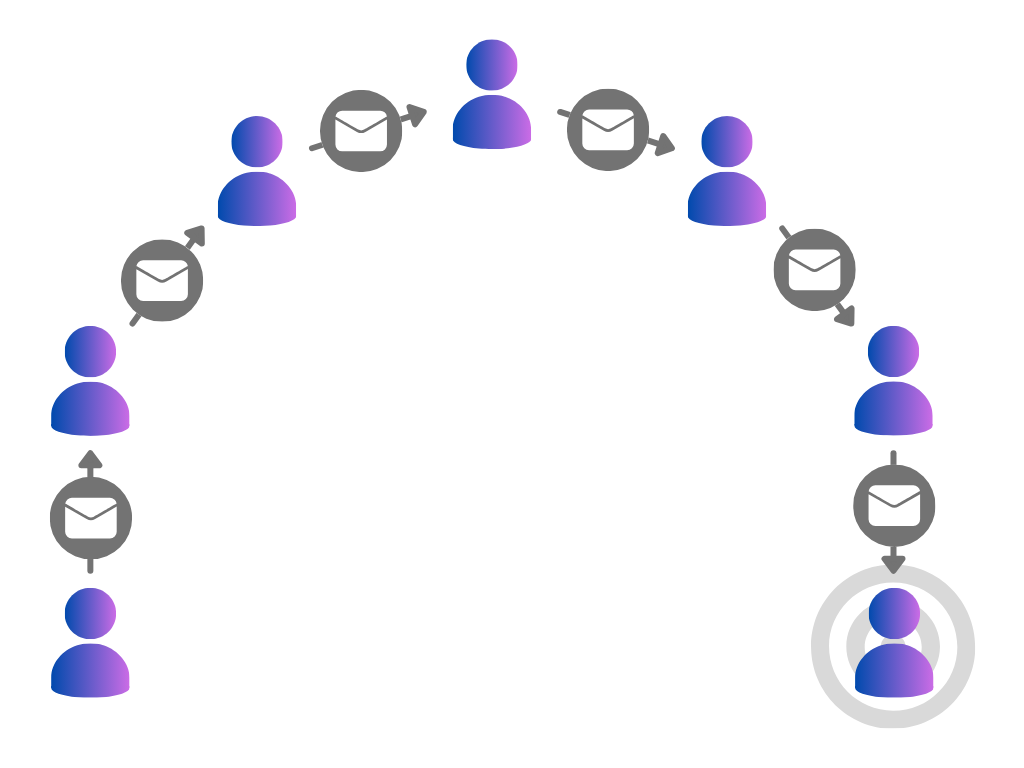
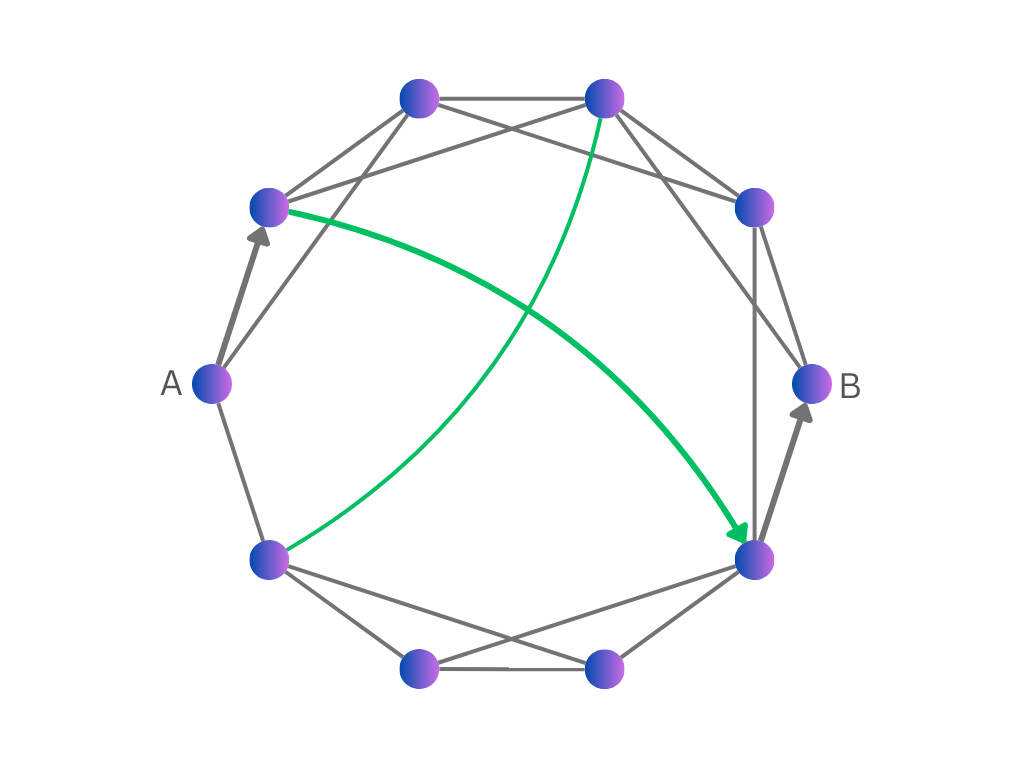
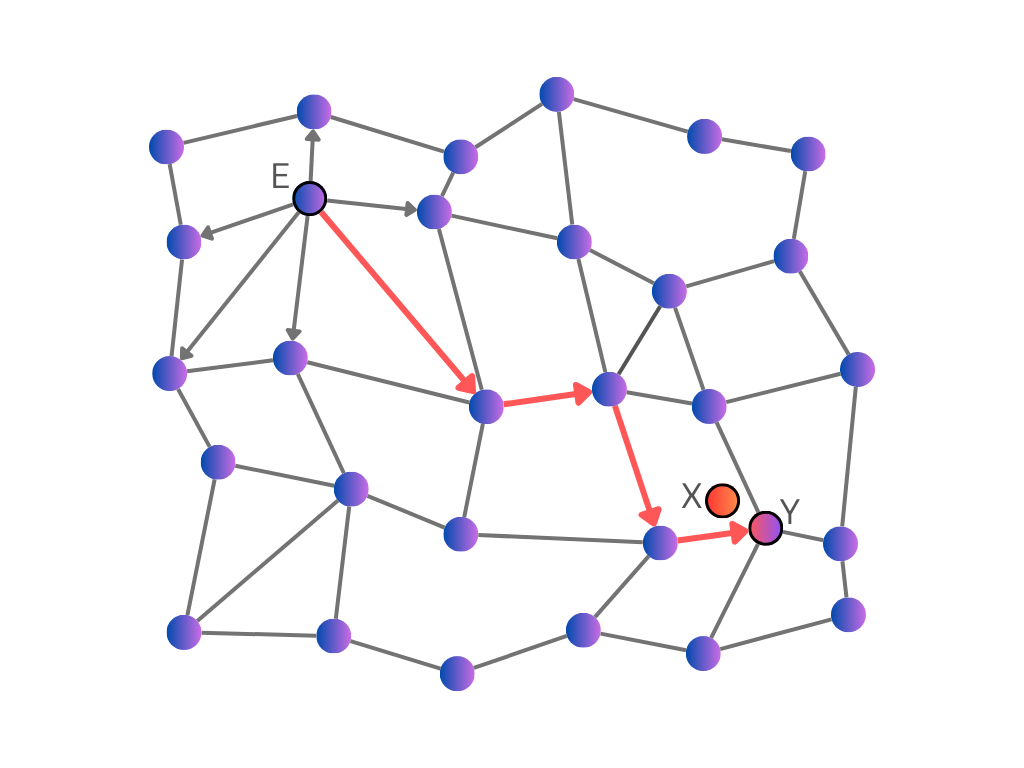

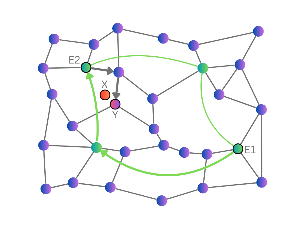

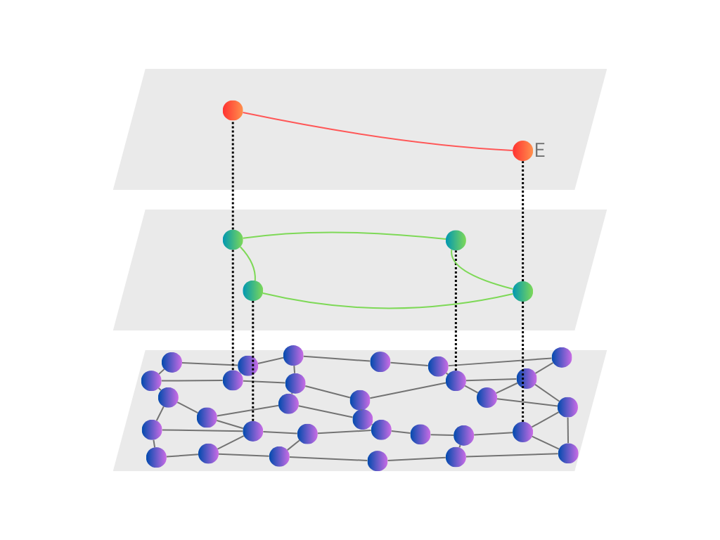


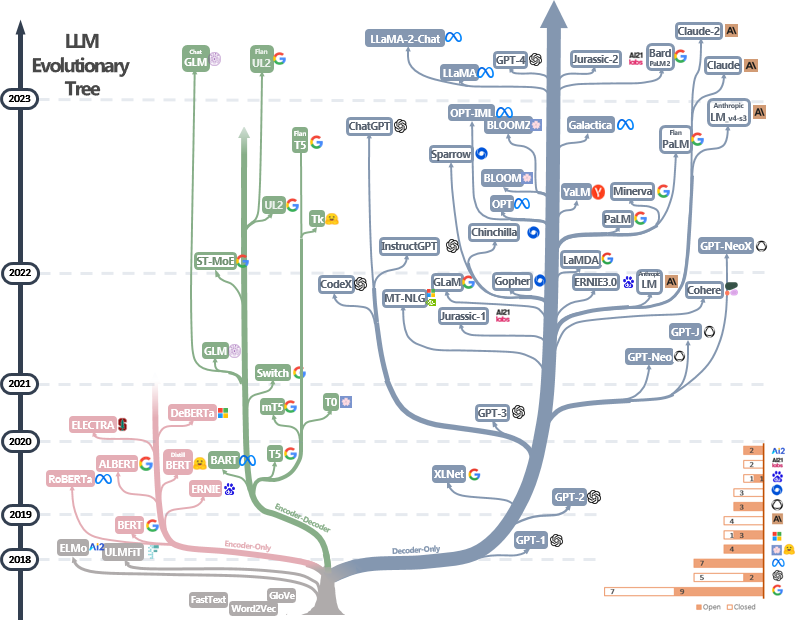

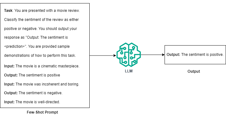
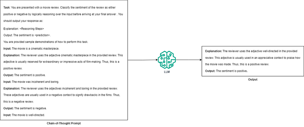
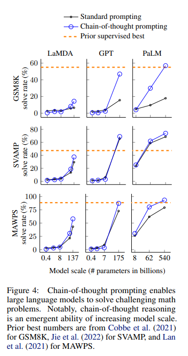
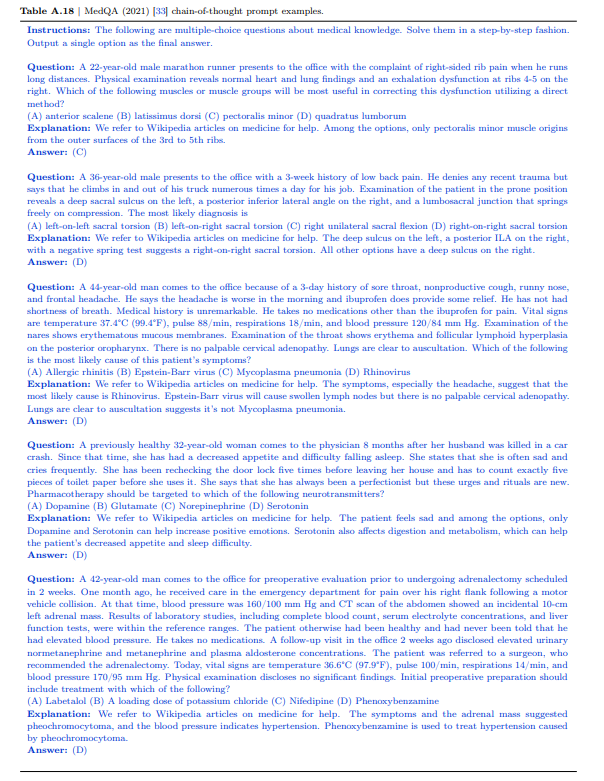
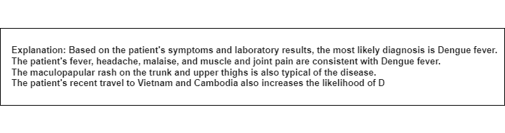
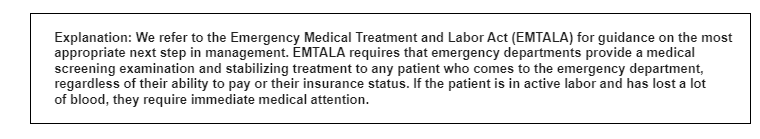

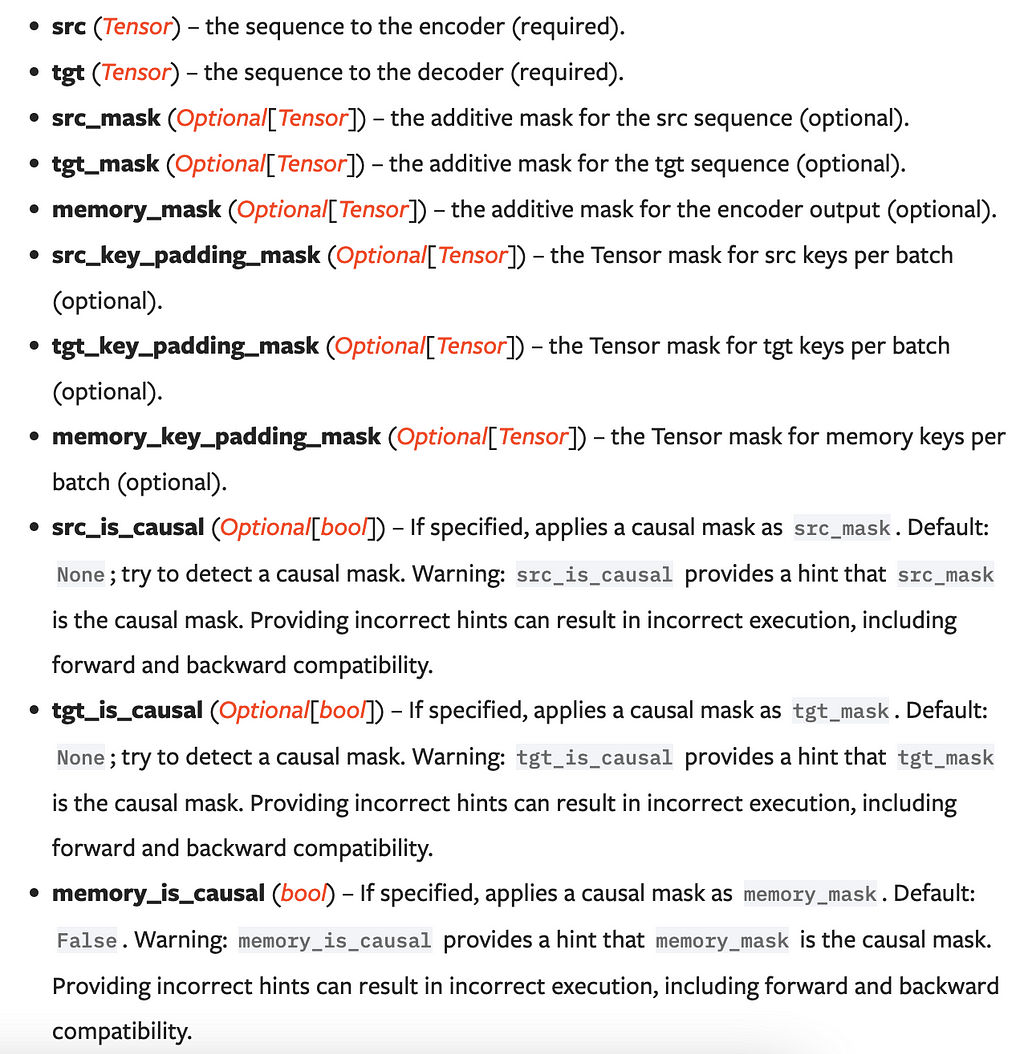
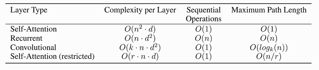
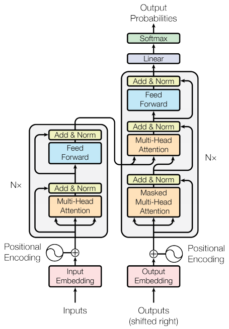
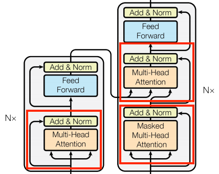
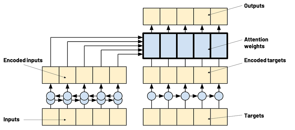
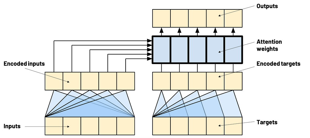
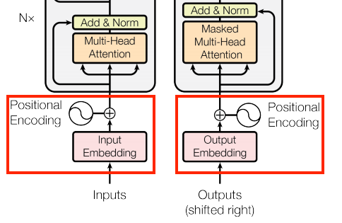
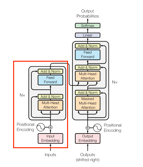
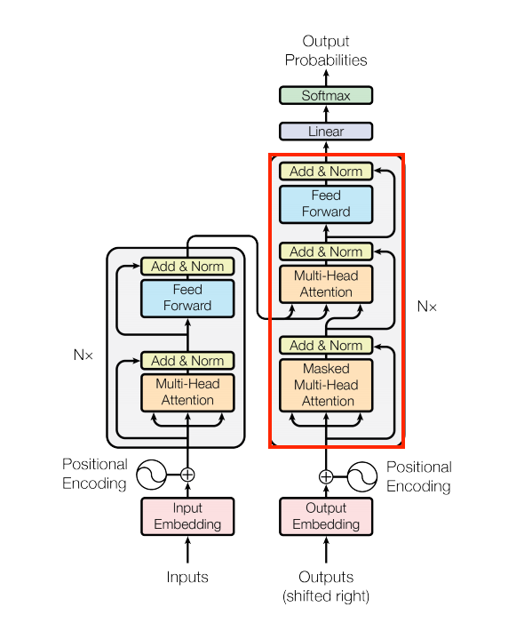
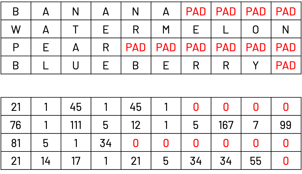
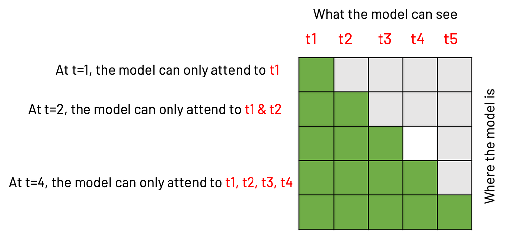
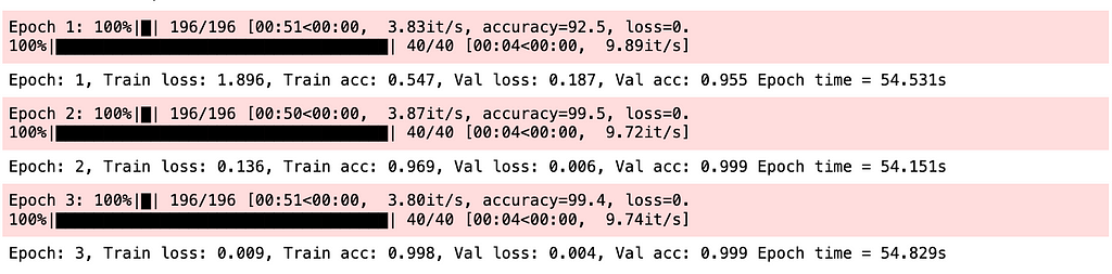
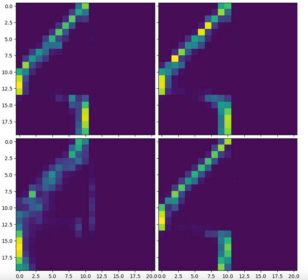
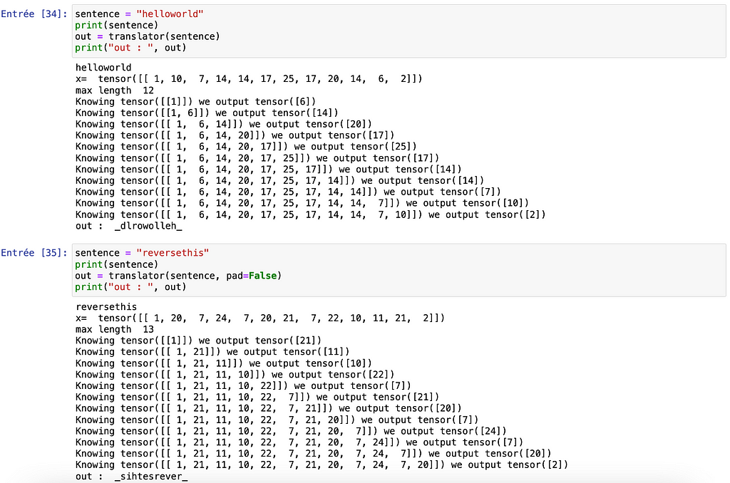
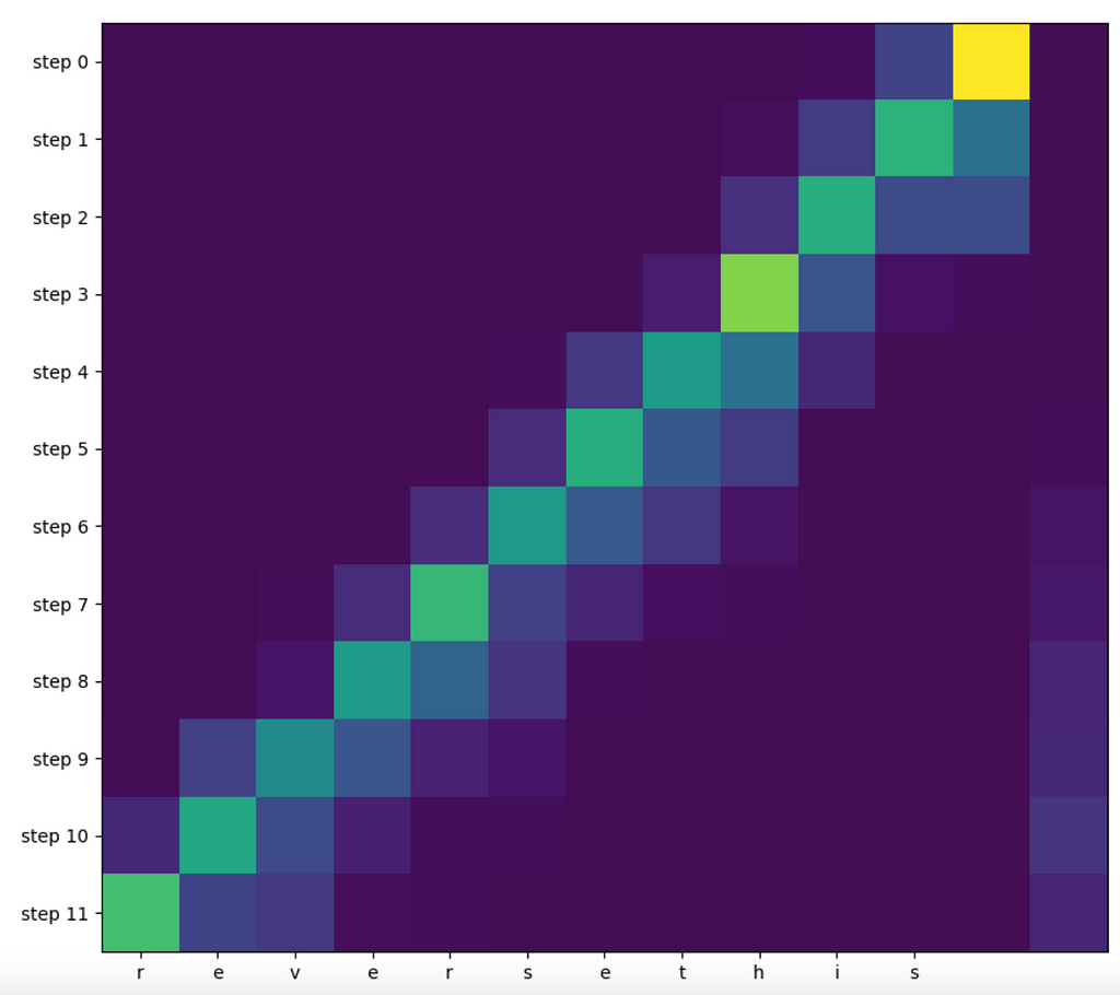


