Category: AI

Vision Transformers Explained Series

The Math and the Code Behind Position Embeddings in Vision Transformers

Since their introduction in 2017 with Attention is All You Need¹, transformers have established themselves as the state of the art for natural language processing (NLP). In 2021, An Image is Worth 16×16 Words² successfully adapted transformers for computer vision tasks. Since then, numerous transformer-based architectures have been proposed for computer vision.

This article examines why position embeddings are a necessary component of vision transformers, and how different papers implement position embeddings. It includes open-source code for positional embeddings, as well as conceptual explanations. All of the code uses the PyTorch Python package.

This article is part of a collection examining the internal workings of Vision Transformers in depth. Each of these articles is also available as a Jupyter Notebook with executable code. The other articles in the series are:

• Vision Transformers, Explained
  → Jupyter Notebook
• Attention for Vision Transformers, Explained
  → Jupyter Notebook
• Position Embeddings for Vision Transformers, Explained
  → Jupyter Notebook
• Tokens-to-Token Vision Transformers, Explained
  → Jupyter Notebook
• GitHub Repository for Vision Transformers, Explained Series

Table of Contents

• Why Use Position Embeddings?
• Attention Invariance Up to Permutation
• Position Embeddings in Literature
• An Example Position Embedding
   — Defining the Position Embedding
   — Applying Position Embedding to Tokens
• Conclusion
   — Further Reading
   — Citations

Why Use Position Embeddings?

Attention is All You Need¹ states that transformers, due to their lack of recurrence or convolution, are not capable of learning information about the order of a set of tokens. Without a position embedding, transformers are invariant to the order of the tokens. For images, that means that patches of an image can be scrambled without impacting the predicted output.

Let’s look at an example of patch order on this pixel art Mountain at Dusk by Luis Zuno (@ansimuz)³. The original artwork has been cropped and converted to a single channel image. This means that each pixel has a value between zero and one. Single channel images are typically displayed in grayscale; however, we’ll be displaying it in a purple color scheme because its easier to see.

mountains = np.load(os.path.join(figure_path, 'mountains.npy'))

H = mountains.shape[0]
W = mountains.shape[1]
print('Mountain at Dusk is H =', H, 'and W =', W, 'pixels.')
print('n')

fig = plt.figure(figsize=(10,6))
plt.imshow(mountains, cmap='Purples_r')
plt.xticks(np.arange(-0.5, W+1, 10), labels=np.arange(0, W+1, 10))
plt.yticks(np.arange(-0.5, H+1, 10), labels=np.arange(0, H+1, 10))
plt.clim([0,1])
cbar_ax = fig.add_axes([0.95, .11, 0.05, 0.77])
plt.clim([0, 1])
plt.colorbar(cax=cbar_ax);
#plt.savefig(os.path.join(figure_path, 'mountains.png'), bbox_inches='tight')

Mountain at Dusk is H = 60 and W = 100 pixels.

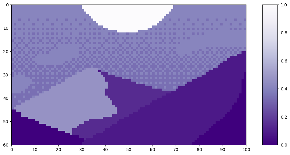
We can split this image up into patches of size 20. (For a more in depth explanation of splitting images into patches, see the Vision Transformers article.)

P = 20
N = int((H*W)/(P**2))
print('There will be', N, 'patches, each', P, 'by', str(P)+'.')
print('n')

fig = plt.figure(figsize=(10,6))
plt.imshow(mountains, cmap='Purples_r')
plt.clim([0,1])
plt.hlines(np.arange(P, H, P)-0.5, -0.5, W-0.5, color='w')
plt.vlines(np.arange(P, W, P)-0.5, -0.5, H-0.5, color='w')
plt.xticks(np.arange(-0.5, W+1, 10), labels=np.arange(0, W+1, 10))
plt.yticks(np.arange(-0.5, H+1, 10), labels=np.arange(0, H+1, 10))
x_text = np.tile(np.arange(9.5, W, P), 3)
y_text = np.repeat(np.arange(9.5, H, P), 5)
for i in range(1, N+1):
    plt.text(x_text[i-1], y_text[i-1], str(i), color='w', fontsize='xx-large', ha='center')
plt.text(x_text[2], y_text[2], str(3), color='k', fontsize='xx-large', ha='center');
#plt.savefig(os.path.join(figure_path, 'mountain_patches.png'), bbox_inches='tight')

There will be 15 patches, each 20 by 20.

The claim is that vision transformers would be unable to distinguish the original image with a version where the patches had been scrambled.

np.random.seed(21)
scramble_order = np.random.permutation(N)
left_x = np.tile(np.arange(0, W-P+1, 20), 3)
right_x = np.tile(np.arange(P, W+1, 20), 3)
top_y = np.repeat(np.arange(0, H-P+1, 20), 5)
bottom_y = np.repeat(np.arange(P, H+1, 20), 5)

scramble = np.zeros_like(mountains)
for i in range(N):
    t = scramble_order[i]
    scramble[top_y[i]:bottom_y[i], left_x[i]:right_x[i]] = mountains[top_y[t]:bottom_y[t], left_x[t]:right_x[t]]
    
fig = plt.figure(figsize=(10,6))
plt.imshow(scramble, cmap='Purples_r')
plt.clim([0,1])
plt.hlines(np.arange(P, H, P)-0.5, -0.5, W-0.5, color='w')
plt.vlines(np.arange(P, W, P)-0.5, -0.5, H-0.5, color='w')
plt.xticks(np.arange(-0.5, W+1, 10), labels=np.arange(0, W+1, 10))
plt.yticks(np.arange(-0.5, H+1, 10), labels=np.arange(0, H+1, 10))
x_text = np.tile(np.arange(9.5, W, P), 3)
y_text = np.repeat(np.arange(9.5, H, P), 5)
for i in range(N):
    plt.text(x_text[i], y_text[i], str(scramble_order[i]+1), color='w', fontsize='xx-large', ha='center')
    
i3 = np.where(scramble_order==2)[0][0]
plt.text(x_text[i3], y_text[i3], str(scramble_order[i3]+1), color='k', fontsize='xx-large', ha='center');
#plt.savefig(os.path.join(figure_path, 'mountain_scrambled_patches.png'), bbox_inches='tight')

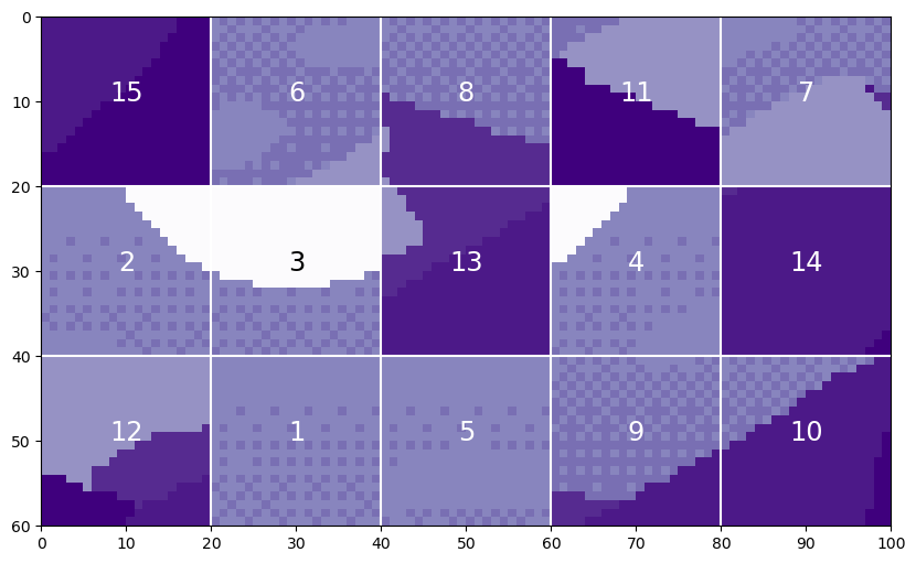
Obviously, this is a very different image from the original, and you wouldn’t want a vision transformer to treat these two images as the same.

Attention Invariance Up to Permutation

Let’s investigate the claim that vision transformers are invariant to the order of the tokens. The component of the transformer that would be invariant to token order is the attention module. While an in depth explanation of the attention module is not the focus of this article, a basis understanding is required. For a more detailed walk through of attention in vision transformers, see the Attention article.

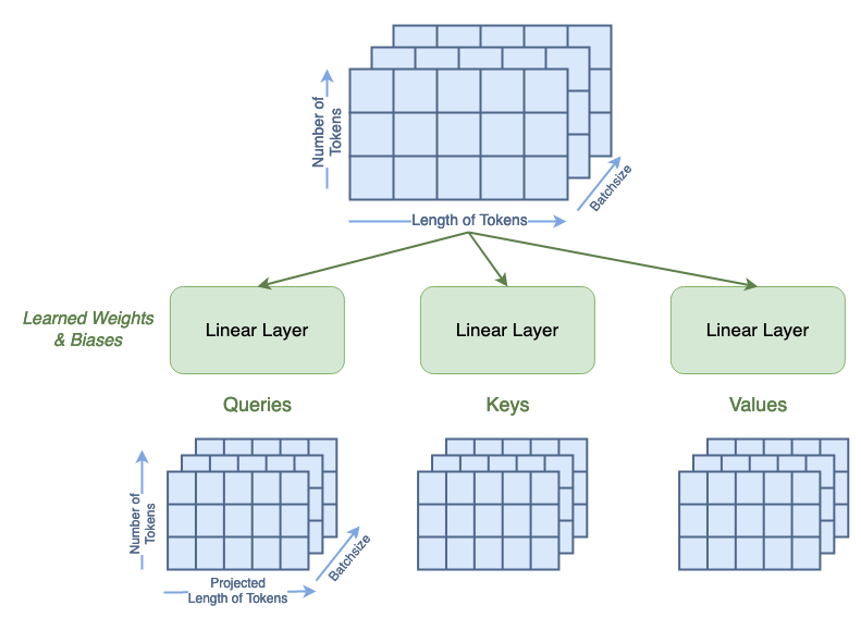
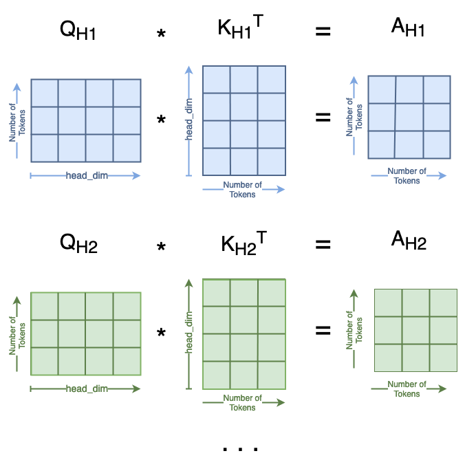
Attention is computed from three matrices — Queries, Keys, and Values — each generated from passing the tokens through a linear layer. Once the Q, K, and V matrices are generated, attention is computed using the following formula.

where Q, K, V, are the queries, keys, and values, respectively; and dₖ is a scaling value. To demonstrate the invariance of attention to token order, we’ll start with three randomly generated matrices to represent Q, K, and V. The shape of Q, K, and V is as follows:

We’ll use 4 tokens of projected length 9 in this example. The matrices will contain integers to avoid floating point multiplication errors. Once generated, we’ll switch the position of token 0 and token 2 in all three matrices. Matrices with swapped tokens will be denoted with a subscript s.

n_tokens = 4
l_tokens = 9
shape = n_tokens, l_tokens
mx = 20 #max integer for generated matricies

# Generate Normal Matricies
np.random.seed(21)
Q = np.random.randint(1, mx, shape)
K = np.random.randint(1, mx, shape)
V = np.random.randint(1, mx, shape)

# Generate Row-Swapped Matricies
swapQ = copy.deepcopy(Q)
swapQ[[0, 2]] = swapQ[[2, 0]]
swapK = copy.deepcopy(K)
swapK[[0, 2]] = swapK[[2, 0]]
swapV = copy.deepcopy(V)
swapV[[0, 2]] = swapV[[2, 0]]

# Plot Matricies
fig, axs = plt.subplots(nrows=3, ncols=2, figsize=(8,8))
fig.tight_layout(pad=2.0)
plt.subplot(3, 2, 1)
mat_plot(Q, 'Q')
plt.subplot(3, 2, 2)
mat_plot(swapQ, r'$Q_S$')
plt.subplot(3, 2, 3)
mat_plot(K, 'K')
plt.subplot(3, 2, 4)
mat_plot(swapK, r'$K_S$')
plt.subplot(3, 2, 5)
mat_plot(V, 'V')
plt.subplot(3, 2, 6)
mat_plot(swapV, r'$V_S$')

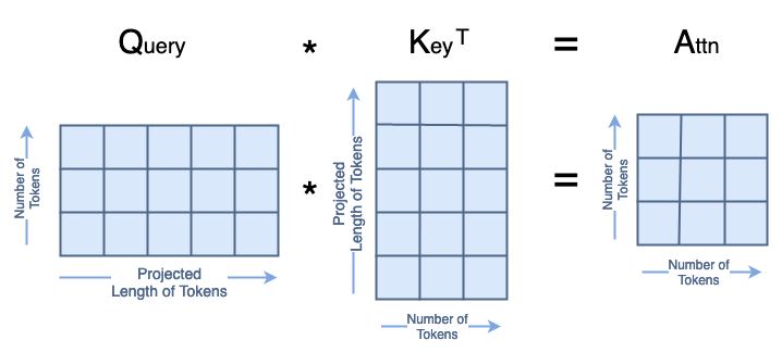
The first matrix multiplication in the attention formula is Q·Kᵀ=A, where the resulting matrix A is a square with size equal to the number of tokens. When we compute Aₛ with Qₛ and Kₛ, the resulting Aₛ has both rows [0, 2] and columns [0,2] swapped from A.

A = Q @ K.transpose()
swapA = swapQ @ swapK.transpose()
modA = copy.deepcopy(A)
modA[[0,2]] = modA[[2,0]] #swap rows
modA[:, [2, 0]] = modA[:, [0, 2]] #swap cols

fig, axs = plt.subplots(nrows=1, ncols=3, figsize=(8,3))
fig.tight_layout(pad=1.0)
plt.subplot(1, 3, 1)
mat_plot(A, r'$A = Q*K^T$')
plt.subplot(1, 3, 2)
mat_plot(swapA, r'$A_S = Q_S * K_S^T$')
plt.subplot(1, 3, 3)
mat_plot(modA, 'Anwith rows [0,2] swapedn and cols [0,2] swaped')

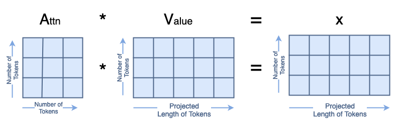
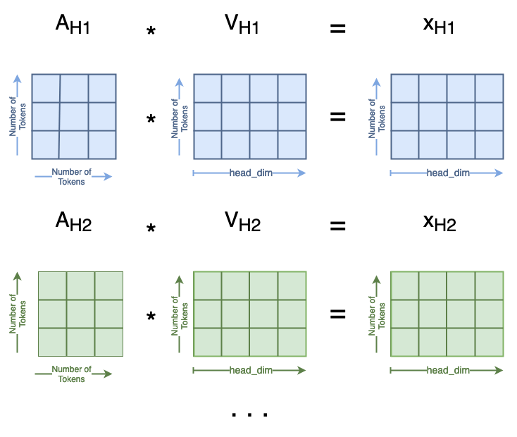
The next matrix multiplication is A·V=A, where the resulting matrix A has the same shape as the initial Q, K, and V matrices. When we compute Aₛ with Aₛ and Vₛ, the resulting Aₛ has rows [0,2] swapped from A.

A = A @ V
swapA = swapA @ swapV
modA = copy.deepcopy(A)
modA[[0,2]] = modA[[2,0]] #swap rows

fig, axs = plt.subplots(nrows=2, ncols=2, figsize=(12, 7))
fig.tight_layout(pad=1.0)
plt.subplot(2, 2, 1)
mat_plot(A, r'$A = A*V$')
plt.subplot(2, 2, 2)
mat_plot(swapA, r'$A_S = A_S * V_S$')
plt.subplot(2, 2, 4)
mat_plot(modA, 'Anwith rows [0,2] swaped')
axs[1,0].axis('off')

This demonstrates that changing the order of the tokens in the input to an attention layer results in an output attention matrix with the same token rows changed. This remains intuitive, as attention is a computation of the relationship between the tokens. Without position information, changing the token order does not change how the tokens are related. It isn’t obvious to me why this permutation of the output isn’t enough information to convey position to the transformers. However, everything I’ve read says that it isn’t enough, so we accept that and move forward.

Position Embeddings in Literature

In addition to the theoretically justification for positional embeddings, models that utilize position embeddings perform with higher accuracy than models without. However, there isn’t clear evidence supporting one type of position embedding over another.

In Attention is All You Need¹, they use a fixed sinusoidal positional embedding. They note that they experimented with a learned positional embedding, but observed “nearly identical results.” Note that this model was designed for NLP applications, specifically translation. The authors proceeded with the fixed embedding because it allowed for varying phrase lengths. This would likely not be a concern in computer vision applications.

In An Image is Worth 16×16 Words², they apply positional embeddings to images. They run ablation studies on four different position embeddings in both fixed and learnable settings. This study encompasses no position embedding, a 1D position embedding, a 2D position embedding, and a relative position embedding. They find that models with a position embedding significantly outperform models without a position embedding. However, there is little difference between their different types of positional embeddings or between the fixed and learnable embeddings. This is congruent with the results in [1] that a position embedding is beneficial, though the exact embedding chosen is of little consequence.

In Tokens-to-Token ViT: Training Vision Transformers from Scratch on ImageNet⁴, they use a sinusoidal position embedding that they describe as being the same as in [2]. Their released code mirrors the equations for the sinusoidal position embedding in [1]. Furthermore, their released code fixes the position embedding rather than letting it be a learned parameter with a sinusoidal initialization.

An Example Position Embedding

Defining the Position Embedding

Now, we can look at the specifics of a sinusoidal position embedding. The code is based on the publicly available GitHub code for Tokens-to-Token ViT⁴. Functionally, the position embedding is a matrix with the same shape as the tokens. This looks like:

The formulae for the sinusoidal position embedding from [1] look like

where PE is the position embedding matrix, i is along the number of tokens, j is along the length of the tokens, and d is the token length.

In code, that looks like

def get_sinusoid_encoding(num_tokens, token_len):
    """ Make Sinusoid Encoding Table

        Args:
            num_tokens (int): number of tokens
            token_len (int): length of a token
            
        Returns:
            (torch.FloatTensor) sinusoidal position encoding table
    """

    def get_position_angle_vec(i):
        return [i / np.power(10000, 2 * (j // 2) / token_len) for j in range(token_len)]

    sinusoid_table = np.array([get_position_angle_vec(i) for i in range(num_tokens)])
    sinusoid_table[:, 0::2] = np.sin(sinusoid_table[:, 0::2])
    sinusoid_table[:, 1::2] = np.cos(sinusoid_table[:, 1::2]) 

    return torch.FloatTensor(sinusoid_table).unsqueeze(0)

Let’s generate an example position embedding matrix. We’ll use 176 tokens. Each token has length 768, which is the default in the T2T-ViT⁴ code. Once the matrix is generated, we can plot it.

PE = get_sinusoid_encoding(num_tokens=176, token_len=768)

fig = plt.figure(figsize=(10, 8))
plt.imshow(PE[0, :, :], cmap='PuOr_r')
plt.xlabel('Along Length of Token')
plt.ylabel('Individual Tokens');
cbar_ax = fig.add_axes([0.95, .36, 0.05, 0.25])
plt.clim([-1, 1])
plt.colorbar(label='Value of Position Encoding', cax=cbar_ax);
#plt.savefig(os.path.join(figure_path, 'fullPE.png'), bbox_inches='tight')

Let’s zoom in to the beginning of the tokens.

fig = plt.figure()
plt.imshow(PE[0, :, 0:301], cmap='PuOr_r')
plt.xlabel('Along Length of Token')
plt.ylabel('Individual Tokens');
cbar_ax = fig.add_axes([0.95, .2, 0.05, 0.6])
plt.clim([-1, 1])
plt.colorbar(label='Value of Position Encoding', cax=cbar_ax);
#plt.savefig(os.path.join(figure_path, 'zoomedinPE.png'), bbox_inches='tight')

It certainly has a sinusoidal structure!

Applying Position Embedding to Tokens

Now, we can add our position embedding to our tokens! We’re going to use Mountain at Dusk³ with the same patch tokenization as above. That will give us 15 tokens of length 20²=400. For more detail about patch tokenization, see the Vision Transformers article. Recall that the patches look like:

fig = plt.figure(figsize=(10,6))
plt.imshow(mountains, cmap='Purples_r')
plt.hlines(np.arange(P, H, P)-0.5, -0.5, W-0.5, color='w')
plt.vlines(np.arange(P, W, P)-0.5, -0.5, H-0.5, color='w')
plt.xticks(np.arange(-0.5, W+1, 10), labels=np.arange(0, W+1, 10))
plt.yticks(np.arange(-0.5, H+1, 10), labels=np.arange(0, H+1, 10))
x_text = np.tile(np.arange(9.5, W, P), 3)
y_text = np.repeat(np.arange(9.5, H, P), 5)
for i in range(1, N+1):
    plt.text(x_text[i-1], y_text[i-1], str(i), color='w', fontsize='xx-large', ha='center')
plt.text(x_text[2], y_text[2], str(3), color='k', fontsize='xx-large', ha='center')
cbar_ax = fig.add_axes([0.95, .11, 0.05, 0.77])
plt.clim([0, 1])
plt.colorbar(cax=cbar_ax);
#plt.savefig(os.path.join(figure_path, 'mountain_patches_w_colorbar.png'), bbox_inches='tight')

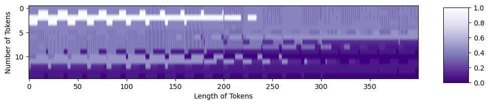
When we convert those patches into tokens, it looks like

tokens = np.zeros((15, 20**2))
for i in range(15):
    patch = gray_mountains[top_y[i]:bottom_y[i], left_x[i]:right_x[i]]
    tokens[i, :] = patch.reshape(1, 20**2)
tokens = tokens.astype(int)
tokens = tokens/255

fig = plt.figure(figsize=(10,6))
plt.imshow(tokens, aspect=5, cmap='Purples_r')
plt.xlabel('Length of Tokens')
plt.ylabel('Number of Tokens')
cbar_ax = fig.add_axes([0.95, .36, 0.05, 0.25])
plt.clim([0, 1])
plt.colorbar(cax=cbar_ax)

Now, we can make a position embedding in the correct shape:

PE = get_sinusoid_encoding(num_tokens=15, token_len=400).numpy()[0,:,:]
fig = plt.figure(figsize=(10,6))
plt.imshow(PE, aspect=5, cmap='PuOr_r')
plt.xlabel('Length of Tokens')
plt.ylabel('Number of Tokens')
cbar_ax = fig.add_axes([0.95, .36, 0.05, 0.25])
plt.clim([0, 1])
plt.colorbar(cax=cbar_ax)

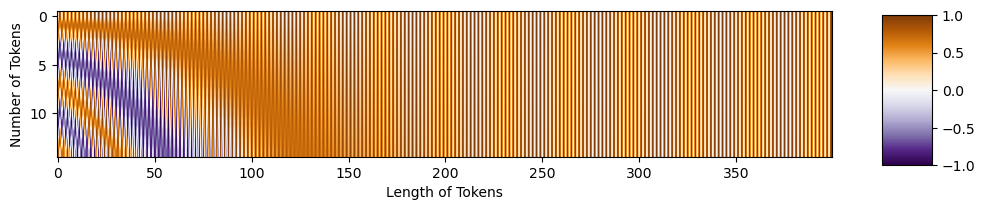
We’re ready now to add the position embedding to the tokens. Purple areas in the position embedding will make the tokens darker, while orange areas will make them lighter.

mountainsPE = tokens + PE
resclaed_mtPE = (position_mountains - np.min(position_mountains)) / np.max(position_mountains - np.min(position_mountains))

fig = plt.figure(figsize=(10,6))
plt.imshow(resclaed_mtPE, aspect=5, cmap='Purples_r')
plt.xlabel('Length of Tokens')
plt.ylabel('Number of Tokens')
cbar_ax = fig.add_axes([0.95, .36, 0.05, 0.25])
plt.clim([0, 1])
plt.colorbar(cax=cbar_ax)

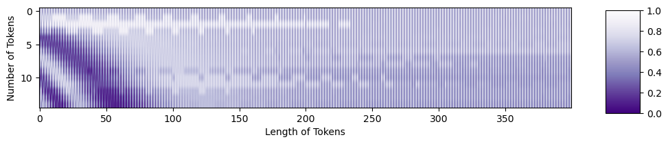
You can see the structure from the original tokens, as well as the structure in the position embedding! Both pieces of information are present to be passed forward into the transformer.

Conclusion

Now, you should have some intuition of how position embeddings help vision transformers learn. The code in this article an be found in the GitHub repository for this series. The code from the T2T-ViT paper⁴ can be found here. Happy transforming!

This article was approved for release by Los Alamos National Laboratory as LA-UR-23–33876. The associated code was approved for a BSD-3 open source license under O#4693.

Further Reading

To learn more about position embeddings in NLP contexts, see

• A Gentle Introduction to Positional Encoding in Transformer Models: https://machinelearningmastery.com/a-gentle-introduction-to-positional-encoding-in-transformer-models-part-1/

For a video lecture broadly about vision transformers (with relevant chapters noted), see

• Vision Transformer and its Applications: https://youtu.be/hPb6A92LROc?si=GaGYiZoyDg0PcdSP
   — Vision Transformer is Invariant to Position of Patches 10:44–12:52 (https://youtu.be/hPb6A92LROc?t=644&si=Keu-5i9BQ5c69mxz)
   — Position Embedding 12:52–14:15 (https://youtu.be/hPb6A92LROc?t=772&si=spdlYZl-TRgbGgzn)

Citations

[1] Vaswani et al (2017). Attention Is All You Need. https://doi.org/10.48550/arXiv.1706.03762

[2] Dosovitskiy et al (2020). An Image is Worth 16×16 Words: Transformers for Image Recognition at Scale. https://doi.org/10.48550/arXiv.2010.11929

[3] Luis Zuno (@ansimuz). Mountain at Dusk Background. License CC0: https://opengameart.org/content/mountain-at-dusk-background

[4] Yuan et al (2021). Tokens-to-Token ViT: Training Vision Transformers from Scratch on ImageNet. https://doi.org/10.48550/arXiv.2101.11986
→ GitHub code: https://github.com/yitu-opensource/T2T-ViT

Position Embeddings for Vision Transformers, Explained was originally published in Towards Data Science on Medium, where people are continuing the conversation by highlighting and responding to this story.

Vision Transformers Explained Series

The Math and the Code Behind Attention Layers in Computer Vision

Since their introduction in 2017 with Attention is All You Need¹, transformers have established themselves as the state of the art for natural language processing (NLP). In 2021, An Image is Worth 16×16 Words² successfully adapted transformers for computer vision tasks. Since then, numerous transformer-based architectures have been proposed for computer vision.

This article takes an in-depth look to how an attention layer works in the context of computer vision. We’ll cover both single-headed and multi-headed attention. It includes open-source code for the attention layers, as well as conceptual explanations of underlying mathematics. The code uses the PyTorch Python package.

This article is part of a collection examining the internal workings of Vision Transformers in depth. Each of these articles is also available as a Jupyter Notebook with executable code. The other articles in the series are:

• Vision Transformers, Explained
  → Jupyter Notebook
• Attention for Vision Transformers, Explained
  → Jupyter Notebook
• Position Embeddings for Vision Transformers, Explained
  → Jupyter Notebook
• Tokens-to-Token Vision Transformers, Explained
  → Jupyter Notebook
• GitHub Repository for Vision Transformers, Explained Series

Table of Contents

• Attention in General
• Single Headed Attention
• Multi-Headed Attention
• Conclusion
   — Further Reading
   — Citations

Attention in General

For NLP applications, attention is often described as the relationship between words (tokens) in a sentence. In a computer vision application, attention looks at the relationships between patches (tokens) in an image.

There are multiple ways to break an image down into a series of tokens. The original ViT² segments an image into patches that are then flattened into tokens; for a more in-depth explanation of this patch tokenization see the Vision Transformers article. The Tokens-to-Token ViT³ develops a more complicated method of creating tokens from an image; more about that methodology can be found in the Tokens-To-Token ViT article.

This article will proceed though an attention layer assuming tokens as input. At the beginning of a transformer, the tokens will be representative of patches in the input image. However, deeper attention layers will compute attention on tokens that have been modified by preceding layers, removing the directness of the representation.

This article examines dot-product (equivalently multiplicative) attention as defined in Attention is All You Need¹. This is the same attention mechanism used in derivative works such as An Image is Worth 16×16 Words² and Tokens-to-Token ViT³. The code is based on the publicly available GitHub code for Tokens-to-Token ViT³ with some modifications. Changes to the source code include, but are not limited to, consolidating the two attention modules into one and implementing multi-headed attention.

The attention module in full is shown below:

class Attention(nn.Module):
    def __init__(self, 
                dim: int,
                chan: int,
                num_heads: int=1,
                qkv_bias: bool=False,
                qk_scale: NoneFloat=None):

        """ Attention Module

            Args:
                dim (int): input size of a single token
                chan (int): resulting size of a single token (channels)
                num_heads(int): number of attention heads in MSA
                qkv_bias (bool): determines if the qkv layer learns an addative bias
                qk_scale (NoneFloat): value to scale the queries and keys by; 
                                    if None, queries and keys are scaled by ``head_dim ** -0.5``
        """

        super().__init__()

        ## Define Constants
        self.num_heads = num_heads
        self.chan = chan
        self.head_dim = self.chan // self.num_heads
        self.scale = qk_scale or self.head_dim ** -0.5
        assert self.chan % self.num_heads == 0, '"Chan" must be evenly divisible by "num_heads".'

        ## Define Layers
        self.qkv = nn.Linear(dim, chan * 3, bias=qkv_bias)
        #### Each token gets projected from starting length (dim) to channel length (chan) 3 times (for each Q, K, V)
        self.proj = nn.Linear(chan, chan)

    def forward(self, x):
        B, N, C = x.shape
        ## Dimensions: (batch, num_tokens, token_len)

        ## Calcuate QKVs
        qkv = self.qkv(x).reshape(B, N, 3, self.num_heads, self.head_dim).permute(2, 0, 3, 1, 4)
        #### Dimensions: (3, batch, heads, num_tokens, chan/num_heads = head_dim)
        q, k, v = qkv[0], qkv[1], qkv[2]

        ## Calculate Attention
        attn = (q * self.scale) @ k.transpose(-2, -1)
        attn = attn.softmax(dim=-1)
        #### Dimensions: (batch, heads, num_tokens, num_tokens)

        ## Attention Layer
        x = (attn @ v).transpose(1, 2).reshape(B, N, self.chan)
        #### Dimensions: (batch, heads, num_tokens, chan)

        ## Projection Layers
        x = self.proj(x)

        ## Skip Connection Layer
        v = v.transpose(1, 2).reshape(B, N, self.chan)
        x = v + x     
        #### Because the original x has different size with current x, use v to do skip connection

        return x

Single-Headed Attention

Starting with only one attention head, let’s step through each line of the forward pass, and look at some matrix diagrams as we go. We’re using 7∗7=49 as our starting token size, since that’s the starting token size in the T2T-ViT models.³ We’re using 64 channels because that’s also the T2T-ViT default³. We’re using 100 tokens because it’s a nice number. We’re using a batch size of 13 because it’s prime and won’t be confused for any of the other parameters.

# Define an Input
token_len = 7*7
channels = 64
num_tokens = 100
batch = 13
x = torch.rand(batch, num_tokens, token_len)
B, N, C = x.shape
print('Input dimensions arentbatchsize:', x.shape[0], 'ntnumber of tokens:', x.shape[1], 'nttoken size:', x.shape[2])

# Define the Module
A = Attention(dim=token_len, chan=channels, num_heads=1, qkv_bias=False, qk_scale=None)
A.eval();

Input dimensions are
   batchsize: 13 
   number of tokens: 100 
   token size: 49

From Attention is All You Need¹, attention is defined in terms of Queries, Keys, and Values matrices. Th first step is to calculate these through a learnable linear layer. The boolean qkv_bias term indicates if these linear layers have a bias term or not. This step also changes the length of the tokens from the input 49 to the chan parameter, which we set as 64.

qkv = A.qkv(x).reshape(B, N, 3, A.num_heads, A.head_dim).permute(2, 0, 3, 1, 4)
q, k, v = qkv[0], qkv[1], qkv[2]
print('Dimensions for Queries arentbatchsize:', q.shape[0], 'ntattention heads:', q.shape[1], 'ntnumber of tokens:', q.shape[2], 'ntnew length of tokens:', q.shape[3])
print('See that the dimensions for queries, keys, and values are all the same:')
print('tShape of Q:', q.shape, 'ntShape of K:', k.shape, 'ntShape of V:', v.shape)

Dimensions for Queries are
   batchsize: 13 
   attention heads: 1 
   number of tokens: 100 
   new length of tokens: 64
See that the dimensions for queries, keys, and values are all the same:
   Shape of Q: torch.Size([13, 1, 100, 64]) 
   Shape of K: torch.Size([13, 1, 100, 64]) 
   Shape of V: torch.Size([13, 1, 100, 64])

Now, we can start to compute attention, which is defined in as:

where Q, K, V, are the queries, keys, and values, respectively; and dₖ is the dimension of the keys, which is equal to the length of the key tokens and equal to the chan length.

We’re going to go through this equation as it is implemented in the code. We’ll call the intermediate matrices Attn.

The first step is to compute:

In the code, we set

By default,

However, the user can specify an alternative scale value as a hyperparameter.

The matrix multiplication Q·Kᵀ in the numerator looks like this:

All of that together in code looks like:

attn = (q * A.scale) @ k.transpose(-2, -1)
print('Dimensions for Attn arentbatchsize:', attn.shape[0], 'ntattention heads:', attn.shape[1], 'ntnumber of tokens:', attn.shape[2], 'ntnumber of tokens:', attn.shape[3])

Dimensions for Attn are
   batchsize: 13 
   attention heads: 1 
   number of tokens: 100 
   number of tokens: 100

Next, we calculate the softmax of A, which doesn’t change it’s shape.

attn = attn.softmax(dim=-1)
print('Dimensions for Attn arentbatchsize:', attn.shape[0], 'ntattention heads:', attn.shape[1], 'ntnumber of tokens:', attn.shape[2], 'ntnumber of tokens:', attn.shape[3])

Dimensions for Attn are
   batchsize: 13 
   attention heads: 1 
   number of tokens: 100 
   number of tokens: 100

Finally, we compute A·V=x, which looks like:

x = attn @ v
print('Dimensions for x arentbatchsize:', x.shape[0], 'ntattention heads:', x.shape[1], 'ntnumber of tokens:', x.shape[2], 'ntlength of tokens:', x.shape[3])

Dimensions for x are
   batchsize: 13 
   attention heads: 1 
   number of tokens: 100 
   length of tokens: 64

The output x is reshaped to remove the attention head dimension.

x = x.transpose(1, 2).reshape(B, N, A.chan)
print('Dimensions for x arentbatchsize:', x.shape[0], 'ntnumber of tokens:', x.shape[1], 'ntlength of tokens:', x.shape[2])

Dimensions for x are
   batchsize: 13 
   number of tokens: 100 
   length of tokens: 64

We then feed x through a learnable linear layer that does not change it’s shape.

x = A.proj(x)
print('Dimensions for x arentbatchsize:', x.shape[0], 'ntnumber of tokens:', x.shape[1], 'ntlength of tokens:', x.shape[2])

Dimensions for x are
   batchsize: 13 
   number of tokens: 100 
   length of tokens: 64

Lastly, we implement a skip connection. Since the current shape of x is different from the input shape of x, we use V for the skip connection. We do flatten V in the attention head dimension.

orig_shape = (batch, num_tokens, token_len)
curr_shape = (x.shape[0], x.shape[1], x.shape[2])
v = v.transpose(1, 2).reshape(B, N, A.chan)
v_shape = (v.shape[0], v.shape[1], v.shape[2])
print('Original shape of input x:', orig_shape)
print('Current shape of x:', curr_shape)
print('Shape of V:', v_shape)
x = v + x     
print('After skip connection, dimensions for x arentbatchsize:', x.shape[0], 'ntnumber of tokens:', x.shape[1], 'ntlength of tokens:', x.shape[2])

Original shape of input x: (13, 100, 49)
Current shape of x: (13, 100, 64)
Shape of V: (13, 100, 64)
After skip connection, dimensions for x are
   batchsize: 13 
   number of tokens: 100 
   length of tokens: 64

That completes the attention layer!

Multi-Headed Attention

Now that we’ve looked at single headed attention, we can expand to multi-headed attention. In the context of computer vision, this is often called Multi-headed Self Attention (MSA). This section isn’t going to go through all the steps in as much detail; instead, we’ll focus on the places where the matrix shapes differ.

Same as for a single attention head, we’re using 7∗7=49 as our starting token size and 64 channels because that’s the T2T-ViT default³. We’re using 100 tokens because it’s a nice number. We’re using a batch size of 13 because it’s prime and won’t be confused for any of the other parameters.

The number of attention heads must evenly divide the number of channels, so for this example we’ll use 4 attention heads.

# Define an Input
token_len = 7*7
channels = 64
num_tokens = 100
batch = 13
num_heads = 4
x = torch.rand(batch, num_tokens, token_len)
B, N, C = x.shape
print('Input dimensions arentbatchsize:', x.shape[0], 'ntnumber of tokens:', x.shape[1], 'nttoken size:', x.shape[2])

# Define the Module
MSA = Attention(dim=token_len, chan=channels, num_heads=num_heads, qkv_bias=False, qk_scale=None)
MSA.eval();

Input dimensions are
   batchsize: 13 
   number of tokens: 100 
   token size: 49

The process to computer the Queries, Keys, and Values remains the same as in single-headed attention. However, you can see that the new length of the tokens is chan/num_heads. The total size of the Q, K, and V matrices have not changed; their contents are just distributed across the head dimension. You can think abut this as segmenting the single headed matrix for the multiple heads:

We’ll denote the submatrices as Qₕᵢ for Query head i.

qkv = MSA.qkv(x).reshape(B, N, 3, MSA.num_heads, MSA.head_dim).permute(2, 0, 3, 1, 4)
q, k, v = qkv[0], qkv[1], qkv[2]
print('Head Dimension = chan / num_heads =', MSA.chan, '/', MSA.num_heads, '=', MSA.head_dim)
print('Dimensions for Queries arentbatchsize:', q.shape[0], 'ntattention heads:', q.shape[1], 'ntnumber of tokens:', q.shape[2], 'ntnew length of tokens:', q.shape[3])
print('See that the dimensions for queries, keys, and values are all the same:')
print('tShape of Q:', q.shape, 'ntShape of K:', k.shape, 'ntShape of V:', v.shape)

Head Dimension = chan / num_heads = 64 / 4 = 16
Dimensions for Queries are
   batchsize: 13 
   attention heads: 4 
   number of tokens: 100 
   new length of tokens: 16
See that the dimensions for queries, keys, and values are all the same:
   Shape of Q: torch.Size([13, 4, 100, 16]) 
   Shape of K: torch.Size([13, 4, 100, 16]) 
   Shape of V: torch.Size([13, 4, 100, 16])

The next step is to compute

for every head i. In this context, the length of the keys is

As in single headed attention, we use the default

though the user can specify an alternative scale value as a hyperparameter.

We end this step with num_heads = 4 different Attn matrices, which looks like:

attn = (q * MSA.scale) @ k.transpose(-2, -1)
print('Dimensions for Attn arentbatchsize:', attn.shape[0], 'ntattention heads:', attn.shape[1], 'ntnumber of tokens:', attn.shape[2], 'ntnumber of tokens:', attn.shape[3])

Dimensions for Attn are
   batchsize: 13 
   attention heads: 4 
   number of tokens: 100 
   number of tokens: 100

Next we calculate the softmax of A, which doesn’t change it’s shape.

Then, we can compute

This is similarly distributed across the multiple attention heads:

attn = attn.softmax(dim=-1)

x = attn @ v
print('Dimensions for x arentbatchsize:', x.shape[0], 'ntattention heads:', x.shape[1], 'ntnumber of tokens:', x.shape[2], 'ntlength of tokens:', x.shape[3])

Dimensions for x are
   batchsize: 13 
   attention heads: 4 
   number of tokens: 100 
   length of tokens: 16

Now we concatenate all of the xₕᵢ’s together through some reshaping. This is the inverse operation from the first step:

x = x.transpose(1, 2).reshape(B, N, MSA.chan)
print('Dimensions for x arentbatchsize:', x.shape[0], 'ntnumber of tokens:', x.shape[1], 'ntlength of tokens:', x.shape[2])

Dimensions for x are
   batchsize: 13 
   number of tokens: 100 
   length of tokens: 64

Now that we’ve concatenated all of the heads back together, the rest of the Attention module remains unchanged. For the skip connection, we still use V, but we have to reshape it to remove the head dimension.

x = MSA.proj(x)
print('Dimensions for x arentbatchsize:', x.shape[0], 'ntnumber of tokens:', x.shape[1], 'ntlength of tokens:', x.shape[2])

orig_shape = (batch, num_tokens, token_len)
curr_shape = (x.shape[0], x.shape[1], x.shape[2])
v = v.transpose(1, 2).reshape(B, N, A.chan)
v_shape = (v.shape[0], v.shape[1], v.shape[2])
print('Original shape of input x:', orig_shape)
print('Current shape of x:', curr_shape)
print('Shape of V:', v_shape)
x = v + x     
print('After skip connection, dimensions for x arentbatchsize:', x.shape[0], 'ntnumber of tokens:', x.shape[1], 'ntlength of tokens:', x.shape[2])

Dimensions for x are
   batchsize: 13 
   number of tokens: 100 
   length of tokens: 64
Original shape of input x: (13, 100, 49)
Current shape of x: (13, 100, 64)
Shape of V: (13, 100, 64)
After skip connection, dimensions for x are
   batchsize: 13 
   number of tokens: 100 
   length of tokens: 64

And that concludes multi-headed attention!

Conclusion

We’ve now walked through every step of an attention layer as implemented for vision transformers. The learnable weights in an attention layer are found in the first projection from tokens to queries, keys, and values and in the final projection. The majority of the attention layer is deterministic matrix multiplication. However, the linear layers can contain large numbers of weights when long tokens are used. The number of weights in the QKV projection layer are equal to input_token_len∗chan∗3, and the number of weights in the final projection layer are equal to chan².

To use the attention layers, you can create custom attention layers (as done here!), or use attention layers included in machine learning packages. If you want to use attention layers as defined here, they can be found in the GitHub repository for this article series. PyTorch also has torch.nn.MultiheadedAttention()⁴ layers, which compute attention as defined above. Happy attending!

This article was approved for release by Los Alamos National Laboratory as LA-UR-23–33876. The associated code was approved for a BSD-3 open source license under O#4693.

Further Reading

To learn more about attention layers in NLP contexts, see

• Transformers Explained Visually Part 1 Overview of Functionality: https://towardsdatascience.com/transformers-explained-visually-part-1-overview-of-functionality-95a6dd460452
• Transformers Explained Visually Part 2 How it Works, Step by Step: https://towardsdatascience.com/transformers-explained-visually-part-2-how-it-works-step-by-step-b49fa4a64f34
• Transformers Explained Visually Part 3 Multi-Headed Attention Deep Dive: https://towardsdatascience.com/transformers-explained-visually-part-3-multi-head-attention-deep-dive-1c1ff1024853
• Visual Guide to Transformer Neural Networks Multi-Head & Self Attention Video: https://www.youtube.com/watch?v=mMa2PmYJlCo

For a video lecture broadly about vision transformers (with relevant chapters noted), see

• Vision Transformer and its Applications: https://youtu.be/hPb6A92LROc?si=GaGYiZoyDg0PcdSP
   — Human Visual Attention: 4:31 — 5:18 (https://youtu.be/hPb6A92LROc?t=271&si=VMx2lM9lvW-oKcW_)
   — Attention as a Dot Product: 5:18–6:14 (https://youtu.be/hPb6A92LROc?t=318&si=pF2SFp2XXjK8AWsL)
   — Description of Attention formula: 16:13–17:52 (https://youtu.be/hPb6A92LROc?si=toAgKQCOh9zGCR-c&t=973)
   — Why Multi-Head Self-Attention: 19:44–19:58 (https://youtu.be/hPb6A92LROc?t=1184&si=Sy1e149ukt99DoRf)

Citations

[1] Vaswani et al (2017). Attention Is All You Need. https://doi.org/10.48550/arXiv.1706.03762

[2] Dosovitskiy et al (2020). An Image is Worth 16×16 Words: Transformers for Image Recognition at Scale. https://doi.org/10.48550/arXiv.2010.11929

[3] Yuan et al (2021). Tokens-to-Token ViT: Training Vision Transformers from Scratch on ImageNet. https://doi.org/10.48550/arXiv.2101.11986
→ GitHub code: https://github.com/yitu-opensource/T2T-ViT

[4] PyTorch. Multiheaded Attention. https://pytorch.org/docs/stable/generated/torch.nn.MultiheadAttention.html

Attention for Vision Transformers, Explained was originally published in Towards Data Science on Medium, where people are continuing the conversation by highlighting and responding to this story.

Vision Transformers Explained Series

A Full Walk-Through of Vision Transformers in PyTorch

Since their introduction in 2017 with Attention is All You Need¹, transformers have established themselves as the state of the art for natural language processing (NLP). In 2021, An Image is Worth 16×16 Words² successfully adapted transformers for computer vision tasks. Since then, numerous transformer-based architectures have been proposed for computer vision.

This article walks through the Vision Transformer (ViT) as laid out in An Image is Worth 16×16 Words². It includes open-source code for the ViT, as well as conceptual explanations of the components. All of the code uses the PyTorch Python package.

This article is part of a collection examining the internal workings of Vision Transformers in depth. Each of these articles is also available as a Jupyter Notebook with executable code. The other articles in the series are:

• Vision Transformers, Explained
  → Jupyter Notebook
• Attention for Vision Transformers, Explained
  → Jupyter Notebook
• Position Embeddings for Vision Transformers, Explained
  → Jupyter Notebook
• Tokens-to-Token Vision Transformers, Explained
  → Jupyter Notebook
• GitHub Repository for Vision Transformers, Explained Series

Table of Contents

• What Are Vision Transformers?
• Model Walk-Through
   — Image Tokenization
  — Token Processing
   — Encoding Block
   — Neural Network Module
   — Prediction Processing
• Complete Code
• Conclusion
   — Further Reading
   — Citations

What are Vision Transformers?

As introduced in Attention is All You Need¹, transformers are a type of machine learning model utilizing attention as the primary learning mechanism. Transformers quickly became the state of the art for sequence-to-sequence tasks such as language translation.

An Image is Worth 16×16 Words² successfully modified the transformer put forth in [1] to solve image classification tasks, creating the Vision Transformer (ViT). The ViT is based on the same attention mechanism as the transformer in [1]. However, while transformers for NLP tasks consist of an encoder attention branch and a decoder attention branch, the ViT only uses an encoder. The output of the encoder is then passed to a neural network “head” that makes a prediction.

The drawback of ViT as implemented in [2] is that it’s optimal performance requires pretraining on large datasets. The best models pretrained on the proprietary JFT-300M dataset. Models pretrained on the smaller, open source ImageNet-21k perform on par with the state-of-the-art convolutional ResNet models.

Tokens-to-Token ViT: Training Vision Transformers from Scratch on ImageNet³ attempts to remove this pretraining requirement by introducing a novel pre-processing methodology to transform an input image into a series of tokens. More about this method can be found here. For this article, we’ll focus on the ViT as implemented in [2].

Model Walk-Through

This article follows the model structure outlined in An Image is Worth 16×16 Words². However, code from this paper is not publicly available. Code from the more recent Tokens-to-Token ViT³ is available on GitHub. The Tokens-to-Token ViT (T2T-ViT) model prepends a Tokens-to-Token (T2T) module to a vanilla ViT backbone. The code in this article is based on the ViT components in the Tokens-to-Token ViT³ GitHub code. Modifications made for this article include, but are not limited to, modifying to allow for non-square input images and removing dropout layers.

A diagram of the ViT model is shown below.

Image Tokenization

The first step of the ViT is to create tokens from the input image. Transformers operate on a sequence of tokens; in NLP, this is commonly a sentence of words. For computer vision, it is less clear how to segment the input into tokens.

The ViT converts an image to tokens such that each token represents a local area — or patch — of the image. They describe reshaping an image of height H, width W, and channels C into N tokens with patch size P:

Each token is of length P²∗C.

Let’s look at an example of patch tokenization on this pixel art Mountain at Dusk by Luis Zuno (@ansimuz)⁴. The original artwork has been cropped and converted to a single channel image. This means that each pixel has a value between zero and one. Single channel images are typically displayed in grayscale; however, we’ll be displaying it in a purple color scheme because its easier to see.

Note that the patch tokenization is not included in the code associated with [3]. All code in this section is original to the author.

mountains = np.load(os.path.join(figure_path, 'mountains.npy'))

H = mountains.shape[0]
W = mountains.shape[1]
print('Mountain at Dusk is H =', H, 'and W =', W, 'pixels.')
print('n')

fig = plt.figure(figsize=(10,6))
plt.imshow(mountains, cmap='Purples_r')
plt.xticks(np.arange(-0.5, W+1, 10), labels=np.arange(0, W+1, 10))
plt.yticks(np.arange(-0.5, H+1, 10), labels=np.arange(0, H+1, 10))
plt.clim([0,1])
cbar_ax = fig.add_axes([0.95, .11, 0.05, 0.77])
plt.clim([0, 1])
plt.colorbar(cax=cbar_ax);
#plt.savefig(os.path.join(figure_path, 'mountains.png'))

Mountain at Dusk is H = 60 and W = 100 pixels.

This image has H=60 and W=100. We’ll set P=20 since it divides both H and W evenly.

P = 20
N = int((H*W)/(P**2))
print('There will be', N, 'patches, each', P, 'by', str(P)+'.')
print('n')

fig = plt.figure(figsize=(10,6))
plt.imshow(mountains, cmap='Purples_r')
plt.hlines(np.arange(P, H, P)-0.5, -0.5, W-0.5, color='w')
plt.vlines(np.arange(P, W, P)-0.5, -0.5, H-0.5, color='w')
plt.xticks(np.arange(-0.5, W+1, 10), labels=np.arange(0, W+1, 10))
plt.yticks(np.arange(-0.5, H+1, 10), labels=np.arange(0, H+1, 10))
x_text = np.tile(np.arange(9.5, W, P), 3)
y_text = np.repeat(np.arange(9.5, H, P), 5)
for i in range(1, N+1):
    plt.text(x_text[i-1], y_text[i-1], str(i), color='w', fontsize='xx-large', ha='center')
plt.text(x_text[2], y_text[2], str(3), color='k', fontsize='xx-large', ha='center');
#plt.savefig(os.path.join(figure_path, 'mountain_patches.png'), bbox_inches='tight'

There will be 15 patches, each 20 by 20.

By flattening these patches, we see the resulting tokens. Let’s look at patch 12 as an example, since it has four different shades in it.

print('Each patch will make a token of length', str(P**2)+'.')
print('n')

patch12 = mountains[40:60, 20:40]
token12 = patch12.reshape(1, P**2)

fig = plt.figure(figsize=(10,1))
plt.imshow(token12, aspect=10, cmap='Purples_r')
plt.clim([0,1])
plt.xticks(np.arange(-0.5, 401, 50), labels=np.arange(0, 401, 50))
plt.yticks([]);
#plt.savefig(os.path.join(figure_path, 'mountain_token12.png'), bbox_inches='tight')

Each patch will make a token of length 400.

After extracting tokens from an image, it is common to use a linear projection to change the length of the tokens. This is implemented as a learnable linear layer. The new length of the tokens is referred to as the latent dimension², channel dimension³, or the token length. After the projection, the tokens are no longer visually identifiable as a patch from the original image.

Now that we understand the concept, we can look at how patch tokenization is implemented in code.

class Patch_Tokenization(nn.Module):
    def __init__(self,
                img_size: tuple[int, int, int]=(1, 1, 60, 100),
                patch_size: int=50,
                token_len: int=768):

        """ Patch Tokenization Module
            Args:
                img_size (tuple[int, int, int]): size of input (channels, height, width)
                patch_size (int): the side length of a square patch
                token_len (int): desired length of an output token
        """
        super().__init__()

        ## Defining Parameters
        self.img_size = img_size
        C, H, W = self.img_size
        self.patch_size = patch_size
        self.token_len = token_len
        assert H % self.patch_size == 0, 'Height of image must be evenly divisible by patch size.'
        assert W % self.patch_size == 0, 'Width of image must be evenly divisible by patch size.'
        self.num_tokens = (H / self.patch_size) * (W / self.patch_size)

        ## Defining Layers
        self.split = nn.Unfold(kernel_size=self.patch_size, stride=self.patch_size, padding=0)
        self.project = nn.Linear((self.patch_size**2)*C, token_len)

    def forward(self, x):
        x = self.split(x).transpose(1,0)
        x = self.project(x)
        return x

Note the two assert statements that ensure the image dimensions are evenly divisible by the patch size. The actual splitting into patches is implemented as a torch.nn.Unfold⁵ layer.

We’ll run an example of this code using our cropped, single channel version of Mountain at Dusk⁴. We should see the values for number of tokens and initial token size as we did above. We’ll use token_len=768 as the projected length, which is the size for the base variant of ViT².

The first line in the code block below is changing the datatype of Mountain at Dusk⁴ from a NumPy array to a Torch tensor. We also have to unsqueeze⁶ the tensor to create a channel dimension and a batch size dimension. As above, we have one channel. Since there is only one image, batchsize=1.

x = torch.from_numpy(mountains).unsqueeze(0).unsqueeze(0).to(torch.float32)
token_len = 768
print('Input dimensions arentbatchsize:', x.shape[0], 'ntnumber of input channels:', x.shape[1], 'ntimage size:', (x.shape[2], x.shape[3]))

# Define the Module
patch_tokens = Patch_Tokenization(img_size=(x.shape[1], x.shape[2], x.shape[3]),
                                    patch_size = P,
                                    token_len = token_len)

Input dimensions are
   batchsize: 1 
   number of input channels: 1 
   image size: (60, 100)

Now, we’ll split the image into tokens.

x = patch_tokens.split(x).transpose(2,1)
print('After patch tokenization, dimensions arentbatchsize:', x.shape[0], 'ntnumber of tokens:', x.shape[1], 'nttoken length:', x.shape[2])

After patch tokenization, dimensions are
   batchsize: 1 
   number of tokens: 15 
   token length: 400

As we saw in the example, there are N=15 tokens each of length 400. Lastly, we project the tokens to be the token_len.

x = patch_tokens.project(x)
print('After projection, dimensions arentbatchsize:', x.shape[0], 'ntnumber of tokens:', x.shape[1], 'nttoken length:', x.shape[2])

After projection, dimensions are
   batchsize: 1 
   number of tokens: 15 
   token length: 768

Now that we have tokens, we’re ready to proceed through the ViT.

Token Processing

We’ll designate the next two steps of the ViT, before the encoding blocks, as “token processing.” The token processing component of the ViT diagram is shown below.

The first step is to prepend a blank token, called the Prediction Token, to the the image tokens. This token will be used at the output of the encoding blocks to make a prediction. It starts off blank — equivalently zero — so that it can gain information from the other image tokens.

We’ll be starting with 175 tokens. Each token has length 768, which is the size for the base variant of ViT². We’re using a batch size of 13 because it’s prime and won’t be confused for any of the other parameters.

# Define an Input
num_tokens = 175
token_len = 768
batch = 13
x = torch.rand(batch, num_tokens, token_len)
print('Input dimensions arentbatchsize:', x.shape[0], 'ntnumber of tokens:', x.shape[1], 'nttoken length:', x.shape[2])

# Append a Prediction Token
pred_token = torch.zeros(1, 1, token_len).expand(batch, -1, -1)
print('Prediction Token dimensions arentbatchsize:', pred_token.shape[0], 'ntnumber of tokens:', pred_token.shape[1], 'nttoken length:', pred_token.shape[2])

x = torch.cat((pred_token, x), dim=1)
print('Dimensions with Prediction Token arentbatchsize:', x.shape[0], 'ntnumber of tokens:', x.shape[1], 'nttoken length:', x.shape[2])

Input dimensions are
   batchsize: 13 
   number of tokens: 175 
   token length: 768
Prediction Token dimensions are
   batchsize: 13 
   number of tokens: 1 
   token length: 768
Dimensions with Prediction Token are
   batchsize: 13 
   number of tokens: 176 
   token length: 768

Now, we add a position embedding for our tokens. The position embedding allows the transformer to understand the order of the image tokens. Note that this is an addition, not a concatenation. The specifics of position embeddings are a tangent best left for another time.

def get_sinusoid_encoding(num_tokens, token_len):
    """ Make Sinusoid Encoding Table

        Args:
            num_tokens (int): number of tokens
            token_len (int): length of a token
            
        Returns:
            (torch.FloatTensor) sinusoidal position encoding table
    """

    def get_position_angle_vec(i):
        return [i / np.power(10000, 2 * (j // 2) / token_len) for j in range(token_len)]

    sinusoid_table = np.array([get_position_angle_vec(i) for i in range(num_tokens)])
    sinusoid_table[:, 0::2] = np.sin(sinusoid_table[:, 0::2])
    sinusoid_table[:, 1::2] = np.cos(sinusoid_table[:, 1::2]) 

    return torch.FloatTensor(sinusoid_table).unsqueeze(0)

PE = get_sinusoid_encoding(num_tokens+1, token_len)
print('Position embedding dimensions arentnumber of tokens:', PE.shape[1], 'nttoken length:', PE.shape[2])

x = x + PE
print('Dimensions with Position Embedding arentbatchsize:', x.shape[0], 'ntnumber of tokens:', x.shape[1], 'nttoken length:', x.shape[2])

Position embedding dimensions are
   number of tokens: 176 
   token length: 768
Dimensions with Position Embedding are
   batchsize: 13 
   number of tokens: 176 
   token length: 768

Now, our tokens are ready to proceed to the encoding blocks.

Encoding Block

The encoding block is where the model actually learns from the image tokens. The number of encoding blocks is a hyperparameter set by the user. A diagram of the encoding block is below.

The code for an encoding block is below.

class Encoding(nn.Module):

    def __init__(self,
       dim: int,
       num_heads: int=1,
       hidden_chan_mul: float=4.,
       qkv_bias: bool=False,
       qk_scale: NoneFloat=None,
       act_layer=nn.GELU, 
       norm_layer=nn.LayerNorm):
        
        """ Encoding Block

            Args:
                dim (int): size of a single token
                num_heads(int): number of attention heads in MSA
                hidden_chan_mul (float): multiplier to determine the number of hidden channels (features) in the NeuralNet component
                qkv_bias (bool): determines if the qkv layer learns an addative bias
                qk_scale (NoneFloat): value to scale the queries and keys by; 
                                    if None, queries and keys are scaled by ``head_dim ** -0.5``
                act_layer(nn.modules.activation): torch neural network layer class to use as activation
                norm_layer(nn.modules.normalization): torch neural network layer class to use as normalization
        """

        super().__init__()

        ## Define Layers
        self.norm1 = norm_layer(dim)
        self.attn = Attention(dim=dim,
                            chan=dim,
                            num_heads=num_heads,
                            qkv_bias=qkv_bias,
                            qk_scale=qk_scale)
        self.norm2 = norm_layer(dim)
        self.neuralnet = NeuralNet(in_chan=dim,
                                hidden_chan=int(dim*hidden_chan_mul),
                                out_chan=dim,
                                act_layer=act_layer)

    def forward(self, x):
        x = x + self.attn(self.norm1(x))
        x = x + self.neuralnet(self.norm2(x))
        return x

The num_heads, qkv_bias, and qk_scale parameters define the Attention module components. A deep dive into attention for vision transformers is left for another time.

The hidden_chan_mul and act_layer parameters define the Neural Network module components. The activation layer can be any torch.nn.modules.activation⁷ layer. We’ll look more at the Neural Network module later.

The norm_layer can be chosen from any torch.nn.modules.normalization⁸ layer.

We’ll now step through each blue block in the diagram and its accompanying code. We’ll use 176 tokens of length 768. We’ll use a batch size of 13 because it’s prime and won’t be confused for any of the other parameters. We’ll use 4 attention heads because it evenly divides token length; however, you won’t see the attention head dimension in the encoding block.

# Define an Input
num_tokens = 176
token_len = 768
batch = 13
heads = 4
x = torch.rand(batch, num_tokens, token_len)
print('Input dimensions arentbatchsize:', x.shape[0], 'ntnumber of tokens:', x.shape[1], 'nttoken length:', x.shape[2])

# Define the Module
E = Encoding(dim=token_len, num_heads=heads, hidden_chan_mul=1.5, qkv_bias=False, qk_scale=None, act_layer=nn.GELU, norm_layer=nn.LayerNorm)
E.eval();

Input dimensions are
   batchsize: 13 
   number of tokens: 176 
   token length: 768

Now, we’ll pass through a norm layer and an Attention module. The Attention module in the encoding block is parameterized so that it don’t change the token length. After the Attention module, we implement our first split connection.

y = E.norm1(x)
print('After norm, dimensions arentbatchsize:', y.shape[0], 'ntnumber of tokens:', y.shape[1], 'nttoken size:', y.shape[2])
y = E.attn(y)
print('After attention, dimensions arentbatchsize:', y.shape[0], 'ntnumber of tokens:', y.shape[1], 'nttoken size:', y.shape[2])
y = y + x
print('After split connection, dimensions arentbatchsize:', y.shape[0], 'ntnumber of tokens:', y.shape[1], 'nttoken size:', y.shape[2])

After norm, dimensions are
   batchsize: 13 
   number of tokens: 176 
   token size: 768
After attention, dimensions are
   batchsize: 13 
   number of tokens: 176 
   token size: 768
After split connection, dimensions are
   batchsize: 13 
   number of tokens: 176 
   token size: 768

Now, we pass through another norm layer, and then the Neural Network module. We finish with the second split connection.

z = E.norm2(y)
print('After norm, dimensions arentbatchsize:', z.shape[0], 'ntnumber of tokens:', z.shape[1], 'nttoken size:', z.shape[2])
z = E.neuralnet(z)
print('After neural net, dimensions arentbatchsize:', z.shape[0], 'ntnumber of tokens:', z.shape[1], 'nttoken size:', z.shape[2])
z = z + y
print('After split connection, dimensions arentbatchsize:', z.shape[0], 'ntnumber of tokens:', z.shape[1], 'nttoken size:', z.shape[2])

After norm, dimensions are
   batchsize: 13 
   number of tokens: 176 
   token size: 768
After neural net, dimensions are
   batchsize: 13 
   number of tokens: 176 
   token size: 768
After split connection, dimensions are
   batchsize: 13 
   number of tokens: 176 
   token size: 768

That’s all for a single encoding block! Since the final dimensions are the same as the initial dimensions, the model can easily pass tokens through multiple encoding blocks, as set by the depth hyperparameter.

Neural Network Module

The Neural Network (NN) module is a sub-component of the encoding block. The NN module is very simple, consisting of a fully-connected layer, an activation layer, and another fully-connected layer. The activation layer can be any torch.nn.modules.activation⁷ layer, which is passed as input to the module. The NN module can be configured to change the shape of an input, or to maintain the same shape. We’re not going to step through this code, as neural networks are common in machine learning, and not the focus of this article. However, the code for the NN module is presented below.

class NeuralNet(nn.Module):
    def __init__(self,
       in_chan: int,
       hidden_chan: NoneFloat=None,
       out_chan: NoneFloat=None,
       act_layer = nn.GELU):
        """ Neural Network Module

            Args:
                in_chan (int): number of channels (features) at input
                hidden_chan (NoneFloat): number of channels (features) in the hidden layer;
                                        if None, number of channels in hidden layer is the same as the number of input channels
                out_chan (NoneFloat): number of channels (features) at output;
                                        if None, number of output channels is same as the number of input channels
                act_layer(nn.modules.activation): torch neural network layer class to use as activation
        """

        super().__init__()

        ## Define Number of Channels
        hidden_chan = hidden_chan or in_chan
        out_chan = out_chan or in_chan

        ## Define Layers
        self.fc1 = nn.Linear(in_chan, hidden_chan)
        self.act = act_layer()
        self.fc2 = nn.Linear(hidden_chan, out_chan)

    def forward(self, x):
        x = self.fc1(x)
        x = self.act(x)
        x = self.fc2(x)
        return x

Prediction Processing

After passing through the encoding blocks, the last thing the model must do is make a prediction. The “prediction processing” component of the ViT diagram is shown below.

We’re going to look at each step of this process. We’ll continue with 176 tokens of length 768. We’ll use a batch size of 1 to illustrate how a single prediction is made. A batch size greater than 1 would be computing this prediction in parallel.

# Define an Input
num_tokens = 176
token_len = 768
batch = 1
x = torch.rand(batch, num_tokens, token_len)
print('Input dimensions arentbatchsize:', x.shape[0], 'ntnumber of tokens:', x.shape[1], 'nttoken length:', x.shape[2])

Input dimensions are
   batchsize: 1 
   number of tokens: 176 
   token length: 768

First, all the tokens are passed through a norm layer.

norm = nn.LayerNorm(token_len)
x = norm(x)
print('After norm, dimensions arentbatchsize:', x.shape[0], 'ntnumber of tokens:', x.shape[1], 'nttoken size:', x.shape[2])

After norm, dimensions are
   batchsize: 1 
   number of tokens: 1001 
   token size: 768

Next, we split off the prediction token from the rest of the tokens. Throughout the encoding block(s), the prediction token has become nonzero and gained information about our input image. We’ll use only this prediction token to make a final prediction.

pred_token = x[:, 0]
print('Length of prediction token:', pred_token.shape[-1])

Length of prediction token: 768

Finally, the prediction token is passed through the head to make a prediction. The head, usually some variety of neural network, is varied based on the model. In An Image is Worth 16×16 Words², they use an MLP (multilayer perceptron) with one hidden layer during pretraining and a single linear layer during fine tuning. In Tokens-to-Token ViT³, they use a single linear layer as a head. This example proceeds with a single linear layer.

Note that the output shape of the head is set based on the parameters of the learning problem. For classification, it is typically a vector of length number of classes in a one-hot encoding. For regression, it would be any integer number of predicted parameters. This example will use an output shape of 1 to represent a single estimated regression value.

head = nn.Linear(token_len, 1)
pred = head(pred_token)
print('Length of prediction:', (pred.shape[0], pred.shape[1]))
print('Prediction:', float(pred))

Length of prediction: (1, 1)
Prediction: -0.5474240779876709

And that’s all! The model has made a prediction!

Complete Code

To create the complete ViT module, we use the Patch Tokenization module defined above and the ViT Backbone module. The ViT Backbone is defined below, and contains the Token Processing, Encoding Blocks, and Prediction Processing components.

class ViT_Backbone(nn.Module):
    def __init__(self,
                preds: int=1,
                token_len: int=768,
                num_heads: int=1,
                Encoding_hidden_chan_mul: float=4.,
                depth: int=12,
                qkv_bias=False,
                qk_scale=None,
                act_layer=nn.GELU,
                norm_layer=nn.LayerNorm):

        """ VisTransformer Backbone
            Args:
                preds (int): number of predictions to output
                token_len (int): length of a token
                num_heads(int): number of attention heads in MSA
                Encoding_hidden_chan_mul (float): multiplier to determine the number of hidden channels (features) in the NeuralNet component of the Encoding Module
                depth (int): number of encoding blocks in the model
                qkv_bias (bool): determines if the qkv layer learns an addative bias
                qk_scale (NoneFloat): value to scale the queries and keys by; 
                 if None, queries and keys are scaled by ``head_dim ** -0.5``
                act_layer(nn.modules.activation): torch neural network layer class to use as activation
                norm_layer(nn.modules.normalization): torch neural network layer class to use as normalization
        """

        super().__init__()

        ## Defining Parameters
        self.num_heads = num_heads
        self.Encoding_hidden_chan_mul = Encoding_hidden_chan_mul
        self.depth = depth

        ## Defining Token Processing Components
        self.cls_token = nn.Parameter(torch.zeros(1, 1, self.token_len))
        self.pos_embed = nn.Parameter(data=get_sinusoid_encoding(num_tokens=self.num_tokens+1, token_len=self.token_len), requires_grad=False)

        ## Defining Encoding blocks
        self.blocks = nn.ModuleList([Encoding(dim = self.token_len, 
                                               num_heads = self.num_heads,
                                               hidden_chan_mul = self.Encoding_hidden_chan_mul,
                                               qkv_bias = qkv_bias,
                                               qk_scale = qk_scale,
                                               act_layer = act_layer,
                                               norm_layer = norm_layer)
             for i in range(self.depth)])

        ## Defining Prediction Processing
        self.norm = norm_layer(self.token_len)
        self.head = nn.Linear(self.token_len, preds)

        ## Make the class token sampled from a truncated normal distrobution 
        timm.layers.trunc_normal_(self.cls_token, std=.02)

    def forward(self, x):
        ## Assumes x is already tokenized

        ## Get Batch Size
        B = x.shape[0]
        ## Concatenate Class Token
        x = torch.cat((self.cls_token.expand(B, -1, -1), x), dim=1)
        ## Add Positional Embedding
        x = x + self.pos_embed
        ## Run Through Encoding Blocks
        for blk in self.blocks:
            x = blk(x)
        ## Take Norm
        x = self.norm(x)
        ## Make Prediction on Class Token
        x = self.head(x[:, 0])
        return x

From the ViT Backbone module, we can define the full ViT model.

class ViT_Model(nn.Module):
 def __init__(self,
    img_size: tuple[int, int, int]=(1, 400, 100),
    patch_size: int=50,
    token_len: int=768,
    preds: int=1,
    num_heads: int=1,
    Encoding_hidden_chan_mul: float=4.,
    depth: int=12,
    qkv_bias=False,
    qk_scale=None,
    act_layer=nn.GELU,
    norm_layer=nn.LayerNorm):

  """ VisTransformer Model

   Args:
    img_size (tuple[int, int, int]): size of input (channels, height, width)
    patch_size (int): the side length of a square patch
    token_len (int): desired length of an output token
    preds (int): number of predictions to output
    num_heads(int): number of attention heads in MSA
    Encoding_hidden_chan_mul (float): multiplier to determine the number of hidden channels (features) in the NeuralNet component of the Encoding Module
    depth (int): number of encoding blocks in the model
    qkv_bias (bool): determines if the qkv layer learns an addative bias
    qk_scale (NoneFloat): value to scale the queries and keys by; 
         if None, queries and keys are scaled by ``head_dim ** -0.5``
    act_layer(nn.modules.activation): torch neural network layer class to use as activation
    norm_layer(nn.modules.normalization): torch neural network layer class to use as normalization
  """
  super().__init__()

  ## Defining Parameters
  self.img_size = img_size
  C, H, W = self.img_size
  self.patch_size = patch_size
  self.token_len = token_len
  self.num_heads = num_heads
  self.Encoding_hidden_chan_mul = Encoding_hidden_chan_mul
  self.depth = depth

  ## Defining Patch Embedding Module
  self.patch_tokens = Patch_Tokenization(img_size,
           patch_size,
           token_len)

  ## Defining ViT Backbone
  self.backbone = ViT_Backbone(preds,
         self.token_len,
         self.num_heads,
         self.Encoding_hidden_chan_mul,
         self.depth,
         qkv_bias,
         qk_scale,
         act_layer,
         norm_layer)
  ## Initialize the Weights
  self.apply(self._init_weights)

 def _init_weights(self, m):
  """ Initialize the weights of the linear layers & the layernorms
  """
  ## For Linear Layers
  if isinstance(m, nn.Linear):
   ## Weights are initialized from a truncated normal distrobution
   timm.layers.trunc_normal_(m.weight, std=.02)
   if isinstance(m, nn.Linear) and m.bias is not None:
    ## If bias is present, bias is initialized at zero
    nn.init.constant_(m.bias, 0)
  ## For Layernorm Layers
  elif isinstance(m, nn.LayerNorm):
   ## Weights are initialized at one
   nn.init.constant_(m.weight, 1.0)
   ## Bias is initialized at zero
   nn.init.constant_(m.bias, 0)
   
 @torch.jit.ignore ##Tell pytorch to not compile as TorchScript
 def no_weight_decay(self):
  """ Used in Optimizer to ignore weight decay in the class token
  """
  return {'cls_token'}

 def forward(self, x):
  x = self.patch_tokens(x)
  x = self.backbone(x)
  return x

In the ViT Model, the img_size, patch_size, and token_len define the Patch Tokenization module.

The num_heads, Encoding_hidden_channel_mul, qkv_bias, qk_scale, and act_layer parameters define the Encoding Bock modules. The act_layer can be any torch.nn.modules.activation⁷ layer. The depth parameter determines how many encoding blocks are in the model.

The norm_layer parameter sets the norm for both within and outside of the Encoding Block modules. It can be chosen from any torch.nn.modules.normalization⁸ layer.

The _init_weights method comes from the T2T-ViT³ code. This method could be deleted to initiate all learned weights and biases randomly. As implemented, the weights of linear layers are initialized as a truncated normal distribution; the biases of linear layers are initialized as zero; the weights of normalization layers are initialized as one; the biases of normalization layers are initialized as zero.

Conclusion

Now, you can go forth and train ViT models with a deep understanding of their mechanics! Below is a list of places to download code for ViT models. Some of them allow for more modifications of the model than others. Happy transforming!

• GitHub Repository for this Article Series
• GitHub Repository for An Image is Worth 16×16 Words²
  → Contains pretrained models and code for fine-tuning; does not contain model definitions
• ViT as implemented in PyTorch Image Models (timm)⁹
  timm.create_model(‘vit_base_patch16_224’, pretrained=True)
• Phil Wang’s vit-pytorch package

This article was approved for release by Los Alamos National Laboratory as LA-UR-23–33876. The associated code was approved for a BSD-3 open source license under O#4693.

Further Reading

To learn more about transformers in NLP contexts, see

• Transformers Explained Visually Part 1 Overview of Functionality: https://towardsdatascience.com/transformers-explained-visually-part-1-overview-of-functionality-95a6dd460452
• Transformers Explained Visually Part 2 How it Works, Step by Step: https://towardsdatascience.com/transformers-explained-visually-part-2-how-it-works-step-by-step-b49fa4a64f34

For a video lecture broadly about vision transformers, see

• Vision Transformer and its Applications: https://youtu.be/hPb6A92LROc?si=GaGYiZoyDg0PcdSP

Citations

[1] Vaswani et al (2017). Attention Is All You Need. https://doi.org/10.48550/arXiv.1706.03762

[2] Dosovitskiy et al (2020). An Image is Worth 16×16 Words: Transformers for Image Recognition at Scale. https://doi.org/10.48550/arXiv.2010.11929

[3] Yuan et al (2021). Tokens-to-Token ViT: Training Vision Transformers from Scratch on ImageNet. https://doi.org/10.48550/arXiv.2101.11986
→ GitHub code: https://github.com/yitu-opensource/T2T-ViT

[4] Luis Zuno (@ansimuz). Mountain at Dusk Background. License CC0: https://opengameart.org/content/mountain-at-dusk-background

[5] PyTorch. Unfold. https://pytorch.org/docs/stable/generated/torch.nn.Unfold.html#torch.nn.Unfold

[6] PyTorch. Unsqueeze. https://pytorch.org/docs/stable/generated/torch.unsqueeze.html#torch.unsqueeze

[7] PyTorch. Non-linear Activation (weighted sum, nonlinearity). https://pytorch.org/docs/stable/nn.html#non-linear-activations-weighted-sum-nonlinearity

[8] PyTorch. Normalization Layers. https://pytorch.org/docs/stable/nn.html#normalization-layers

[9] Ross Wightman. PyTorch Image Models. https://github.com/huggingface/pytorch-image-models

Vision Transformers, Explained was originally published in Towards Data Science on Medium, where people are continuing the conversation by highlighting and responding to this story.

Common mistakes to avoid when you transition from statistical modelling to Machine Learning

My Story

Data Science, Machine Learning, and AI are undeniably buzzwords of today. My LinkedIn is flooded with data gurus sharing learning roadmaps for those eager to break into this data space.

Yet, from my personal experience, I’ve found that the journey towards Data Science isn’t as linear as merely following a fixed roadmap, especially for individuals transitioning from various professional backgrounds. Data Science requires a blend of diverse skills like programming, statistics, math, analytics, soft skills, and domain knowledge. This means that everyone picks up learning from different points depending on their prior experience/skill sets.

As someone who worked in research and analytics for years and pursued a master’s degree in analytics, I have acquired a fair amount of statistical knowledge and its applications. Even then, data science is such a broad and dynamic industry that my knowledge is still all over the place. I struggled to find resources that could effectively fill my knowledge gap between statistics and ML as well. This posed significant challenges to my learning experience.

In this article, I aim to share the technical oversights I encounter as I navigate from research & analytics to data science. Hopefully, my sharing can save you time and help you avoid these pitfalls.

Statistical Modelling Vs Machine Learning

So, you might be wondering why I am starting with a reflection on my journey instead of getting to the point. Well, the reason is simple — I have noticed that many individuals claim to be building ML models when, in reality, they are only crafting statistical models. I confess I was one of them! It’s not like one is better than the other, but I believe it is crucial to recognise the nuances between statistical modelling and ML before I talk about technicalities.

The purpose of statistical models is for making inferences, while the primary goal of Machine Learning is for predictions. Simply put, the ML model leverages statistics and math to generate predictions applicable to real-world scenarios. This is where data splitting and data leakage come into the picture, particularly in the context of supervised Machine Learning.

My initial belief was that understanding statistical analysis was sufficient for prediction tasks. However, I quickly realised that without knowledge of data preparation techniques such as proper data splitting and awareness of potential pitfalls like data leakage, even the most sophisticated statistical models fall short in predictive performance.

So, let’s get started!

Mistake 1: Improper Data Splitting

What is meant by data splitting?

Data splitting, in essence, is dividing your dataset into parts for optimal predictive performance of the model.

Consider a simple OLS regression concept that is familiar to many of us. We all have heard about it in one of the business/stats/finance, economics, or engineering lectures. It is a fundamental ML technique.

Let’s say we have a housing price dataset along with the factors that might affect housing prices.

In traditional statistical analysis, we employ the entire dataset to develop a regression model, as our goal is just to understand what factors influence housing prices. In other words, regression models can explain what degree of changes in prices are associated with the predictors.

However, in ML, the statistical part remains the same, but data splitting becomes crucial. Let me explain why — imagine we train the model on the entire set; how would we know the predictive performance of the model on unseen data?

For this very reason, we typically split the dataset into two sets: training and test sets. The idea is to train the model on one set and evaluate its performance on the other set. Essentially, the test set should serve as real-world data, meaning the model should not have access to the test data in any way throughout the training phase.

Here comes the pitfall that I wasn’t aware of before. Splitting data into two sets is not inherently wrong, but there is a risk of creating an unreliable model. Imagine you train the model on the training set, validate its accuracy on the test set, and then repeat the process to fine-tune the model. This creates a bias in model selection and defeats the whole purpose of “unseen data” because test data was seen multiple times during model development. It undermines the model’s ability to genuinely predict the unseen data, leading to overfitting issues.

How to prevent it:

Ideally, the dataset should be divided into two blocks (three distinct splits):

• ( Training set + Validation set) → 1st block
• Test set → 2nd block

The model can be trained and validated on the 1st block. The 2nd block (the test set) should not be involved in any of the model training processes. Think of the test set as a danger zone!

How you want to split the data is dependent on the size of the dataset. The industry standard is 60% — 80 % for the training set (1st block) and 20% — 40% for the test set. The validation set is normally curved out of the 1st block so the actual training set would be 70% — 90% out of the 1st block , and the rest is for the validation set.

The best way to grasp this concept is through a visual:

There is more than one data-splitting technique other than LOOV (in the picture):

• K-fold Cross-validation, which divides the data into a number of ‘K’ folds and iterates the training processes accordingly
• Rolling Window Cross-validation (for time-series data)
• Blocked Cross-validation (for time-series data)
• Stratified Sampling Splitting for imbalanced classes

Note: Time series data needs extra caution when splitting data due to its temporal order. Randomly splitting the dataset can mess up its time order. (I learnt it the hard way)

The most important thing is regardless of the techniques you use, the “test set” should be kept separate and untouched until the model selection.

Mistake 2: Data Leakage

“In Machine learning, Data Leakage refers to a mistake that is made by the creator of a machine learning model in which they accidentally share the information between the test and training data sets.” — Analytics Vidhya

This is connected to my first point about test data being contaminated by training data. It’s one example of data leakage. However, having a validation set alone can’t avoid data leakage.

In order to prevent data leakage, we need to be careful with the data handling process — from Exploratory Data Analysis (EDA) to Feature Engineering. Any procedure that allows the training data to interact with the test data could potentially lead to leakage.

There are two main types of leakage:

1. Train-test-contamination

A common mistake I made involved applying a standardisation/pre-processing procedure to the entire set before data splitting. For example, using mean imputation to handle missing values/ outliers on the whole dataset. This makes the training data incorporate information from the test data. As a result, the model’s accuracy is inflated compared to its real-life performance.

2. Target leakage

If the features (predictors) have some dependency on the variable that we want to predict (target), or if the features data will not be available at the time of prediction, this can result in target leakage.

Let’s look at the data I worked on as an example. Here, I was trying to predict sales performance based on advertising campaigns. I tried to include the conversion rates. I overlooked the fact that conversion rates are only known post-campaign. In other words, I won’t have this information at the time of forecasting. Plus, because conversion rates are tied to sales data, this introduces a classic case of target leakage. Including conversion rates would lead the model to learn from data that would not be normally accessible, resulting in overly optimistic predictions.

How to prevent data leakage:

In summary, keep these points in mind to address data leakage issues:

1. Proper Data Preprocessing
2. Cross-validation with care
3. Careful Feature Selection

Closing Thoughts

That’s about it! Thanks for sticking with me till the end! I hope this article clarifies the common misconceptions around data splitting and sheds light on the best practices in building efficient ML models.

This is not just for documenting my learning journey but also for mutual learning. So, if you spot a gap in my technical know-how or have any insights to share, feel free to drop me a message!

References:

Daniel Lee Datainterview.com LinkedIn Post

Kaggle — Data Leakage Explanation

Analytics Vidhya — Data Leakage And Its Effect On The Performance of An ML Model

Forecasting: Principles and Practice

Lessons From My ML Journey: Data Splitting and Data Leakage was originally published in Towards Data Science on Medium, where people are continuing the conversation by highlighting and responding to this story.