Discover design approaches for building a scalable information retrieval system
Introduction
Question-answering applications have intensely emerged in recent years. They can be found everywhere: in modern search engines, chatbots or applications that simply retrieve relevant information from large volumes of thematic data.
As the name indicates, the objective of QA applications is to retrieve the most suitable answer to a given question in a text passage. Some of the first methods consisted of naive search by keywords or regular expressions. Obviously, such approaches are not optimal: a question or text can contain typos. Moreover, regular expressions cannot detect synonyms which can be highly relevant to a given word in a query. As a result, these approaches were replaced by the new robust ones, especially in the era of Transformers and vector databases.
This article covers three main design approaches for building modern and scalable QA applications.
Types of QA system architectures
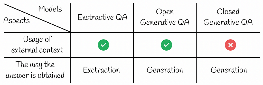
Exctractive QA
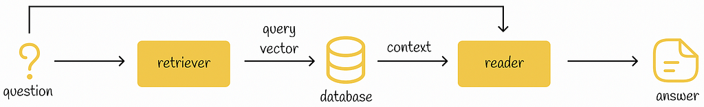
Extractive QA systems consist of three components:
Retriever
Database
Reader
Extractive QA architecture
Firstly, the question is fed into the retriever. The goal of the retriever is to return an embedding corresponding to the question. There can be multiple implementations of retriever starting from simple vectorization methods like TF-IDF, BM-25 and ending up with more complex models. Most of the time, Transformer-like models (BERT) are integrated into the retriever. Unlike naive approaches that rely only on word frequency, language models can build dense embeddings that are capable of capturing the semantic meaning of text.
After obtaining a query vector from a question, it is then used to find the most similar vectors among an external collection of documents. Each of the documents has a certain chance of containing the answer to the question. As a rule, the collection of documents is processed during the training phase by being passed to the retriever which outputs corresponding embeddings to the documents. These embeddings are then usually stored in a database which can provide an effective search.
In QA systems, vector databases usually play the role of a component for efficient storage and search among embeddings based on their similarity. The most popular vector databases are Faiss, Pinecone and Chroma.
If you would like to better understand how vector databases work under the hood, then I recommend you check my article series on similarity search where I deeply cover the most popular algorithms:
By retrieving the k most similar database vectors to the query vector, their original text representations are used to find the answer by another component called the reader. The reader takes an initial question and for each of the k retrieved documents it extracts the answer in the text passage and returns a probability of this answer being correct. The answer with the highest probability is then finally returned from the exclusive QA system.
Fine-tuned large language models specialising in QA downstream tasks are usually used in the role of the reader.
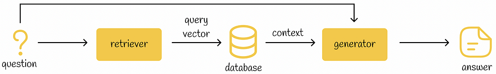
Open Generative QA
Open Generative QA follows exactly the same framework as Extractive QA except for the fact that they use the generator instead of the reader. Unlike the reader, the generator does not extract the answer from a text passage. Instead, the answer is generated from the information provided in the question and text passages. As in the case of Extractive QA, the answer with the highest probability is chosen as the final answer.
As the name indicates, Open Generative QA systems normally use generative models like GPT for answer generation.
Open Generative QA architecture
By having a very similar structure, there might come a question of when it is better to use an Extractive or Open Generative architecture. It turns out that when a reader model has direct access to a text passage containing relative information, it is usually smart enough to retrieve a precise and concise answer. On the other hand, most of the time, generative models tend to produce longer and more generic information for a given context. That might be beneficial in cases when a question is asked in an open form but not for situations when a short or exact answer is expected.
Retrieval-Augmented Generation
Recently, the popularity of the term “Retrieval-Augmented Generation” or “RAG” has skyrocketed in machine learning. In simple words, it is a framework for creating LLM applications whose architecture is based on Open Generative QA systems.
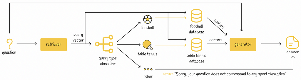
In some cases, if an LLM application works with several knowledge domains, the RAG retriever can add a supplementary step in which it will try to identify the most relevant knowledge domain to a given query. Depending on an identified domain, the retriever can then perform different actions. For example, it is possible to use several vector databases each corresponding to a particular domain. When a query belongs to a certain domain, the vector database of that domain is then used to retrieve the most relevant information for the query.
This technique makes the search process faster since we search through only a particular subset of documents (instead of all documents). Moreover, it can make the search more reliable as the ultimate retrieved context is constructed from more relevant documents.
Example of RAG pipeline. The retriever constructs an embedding from a given question. Then this embedding is used to classify the question into one of the sport categories. For each sport type, the respective vector database is used to retrieve the most similar context. The question and the retrieved context are fed into the generator to produce the answer. If the question was not related to sport, then the RAG application would inform the user about it.
Closed Generative QA
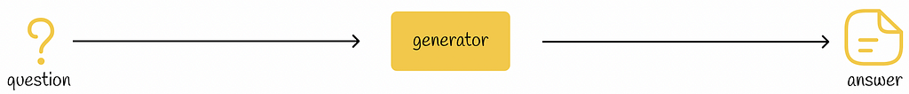
Closed Generative QA systems do not have access to any external information and generate answers by only using the information from the question.
Closed Generative QA architecture
The obvious advantage of closed QA systems is reduced pipeline time as we do not have to search through a large collection of external documents. But it comes with the cost of training and accuracy: the generator should be robust enough and have a large training knowledge to be capable of generating appropriate answers.
Closed Generative QA pipeline has another disadvantage: generators do not know any information that appeared later in the data it had been trained on. To eliminate this issue, a generator can be trained again on a more recent dataset. However, generators usually have millions or billions of parameters, thus training them is an extremely resource-heavy task. In comparison, dealing with the same problem with Extractive QA and Open Generative QA systems is much simpler: it is just enough to add new context data to the vector database.
Most of the time closed generative approach is used in applications with generic questions. For very specific domains, the performance of closed generative models tends to degrade.
Conclusion
In this article, we have discovered three main approaches for building QA systems. There is no absolute winner among them: all of them have their own pros and cons. For that reason, it is firstly necessary to analyse the input problem and then choose the correct QA architecture type, so it can produce a better performance.
It is worth noting that Open Generative QA architecture is currently on the trending hype in machine learning, especially with innovative RAG techniques that have appeared recently. If you are an NLP engineer, then you should definitely keep your eye on RAG systems as they are evolving at a very high rate nowadays.
This is a guest post written by Axfood AB. In this post, we share how Axfood, a large Swedish food retailer, improved operations and scalability of their existing artificial intelligence (AI) and machine learning (ML) operations by prototyping in close collaboration with AWS experts and using Amazon SageMaker. Axfood is Sweden’s second largest food retailer, […]
A Full Walk-Through of the Tokens-to-Token Vision Transformer, and Why It’s Better than the Original
Since their introduction in 2017 with Attention is All You Need¹, transformers have established themselves as the state of the art for natural language processing (NLP). In 2021, An Image is Worth 16×16 Words² successfully adapted transformers for computer vision tasks. Since then, numerous transformer-based architectures have been proposed for computer vision.
In 2021, Tokens-to-Token ViT: Training Vision Transformers from Scratch on ImageNet³ outlined the Tokens-to-Token (T2T) ViT. This model aims to remove the heavy pretraining requirement present in the original ViT². This article walks through the T2T-ViT, including open-source code for T2T-ViT, as well as conceptual explanations of the components. All of the code uses the PyTorch Python package.
This article is part of a collection examining the internal workings of Vision Transformers in depth. Each of these articles is also available as a Jupyter Notebook with executable code. The other articles in the series are:
The first vision transformers able to match the performance of CNNs on computer vision tasks required pre-training on large datasets and then transferring to the benchmark of interest². However, pre-training on such datasets is not always feasible. For one, the pre-training dataset that achieved the best results in An Image is Worth 16×16 Words (the JFT-300M dataset) is not publicly available². Furthermore, vistransformers designed for tasks other than traditional image classification may not have such large pre-training datasets available.
In 2021, Tokens-to-Token ViT: Training Vision Transformers from Scratch on ImageNet³ was published, presenting a methodology that would circumvent the heavy pre-training requirement of previous vistransformers. They achieved this by replacing the patch tokenization in the ViT model² with the a Tokens-to-Token (T2T) module.
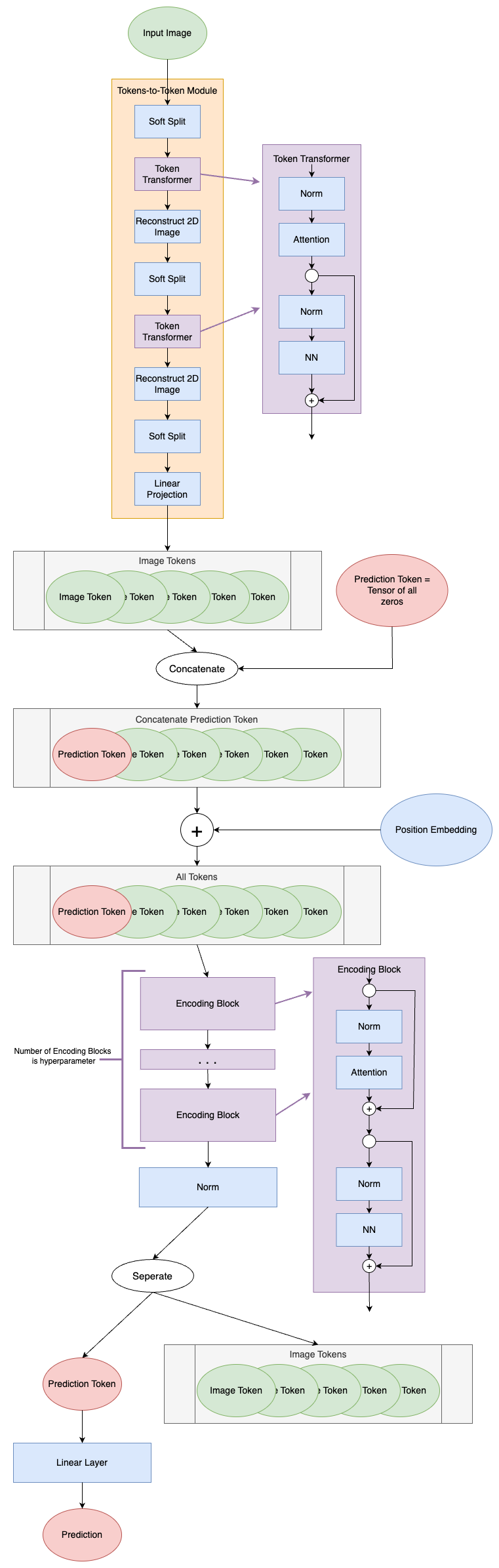
T2T-ViT Model Diagram (image by author)
Since the T2T module is what makes the T2T-ViT model unique, it will be the focus of this article. For a deep dive into the ViT components see the Vision Transformers article. The code is based on the publicly available GitHub code for Tokens-to-Token ViT³ with some modifications. Changes to the source code include, but are not limited to, modifying to allow for non-square input images and removing dropout layers.
Tokens-to-Token (T2T) Module
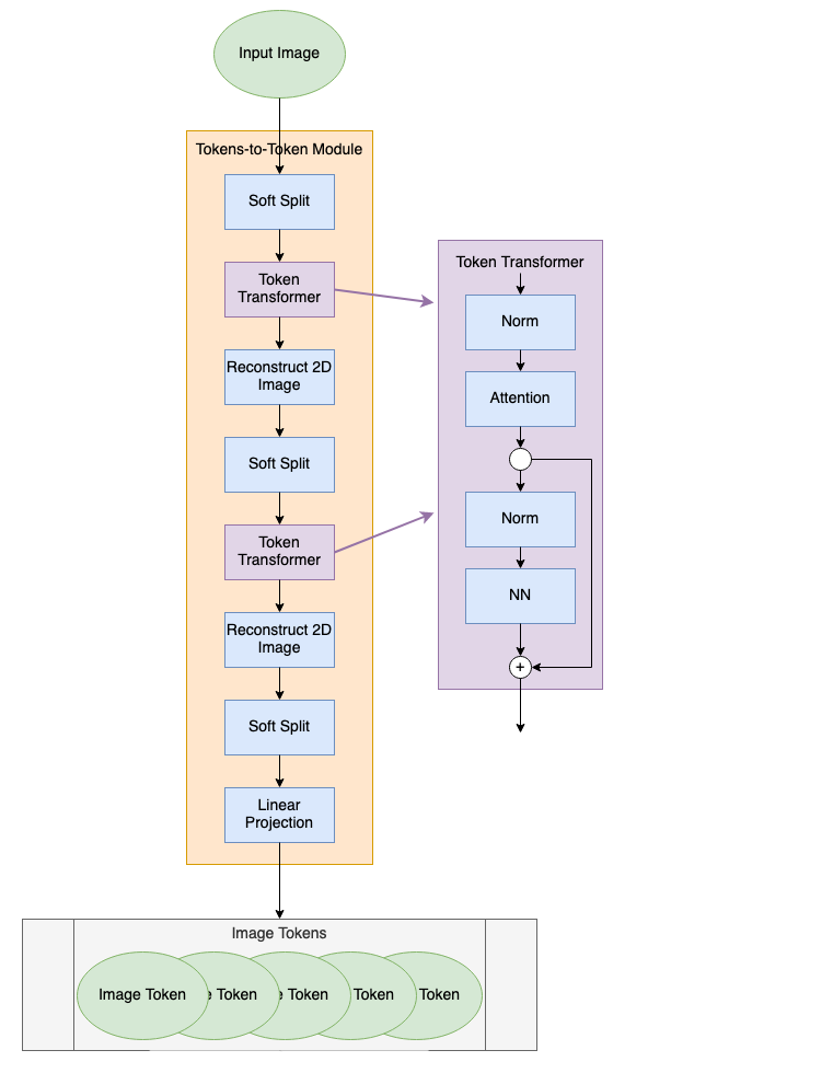
The T2T module serves to process the input image into tokens that can be used in the ViT module. Instead of simply splitting the input image into patches that become tokens, the T2T module sequentially computes attention between tokens and aggregates them together to capture additional structure in the image and to reduce the overall token length. The T2T module diagram is shown below.
T2T Module Diagram (image by author)
Soft Split
As the first layer in the T2T-ViT model, the soft split layer is what separates an image into a series of tokens. The soft split layers are shown as blue blocks in the T2T diagram. Unlike the patch tokenization in the original ViT (read more about that here), the soft splits in the T2T-ViT create overlapping patches.
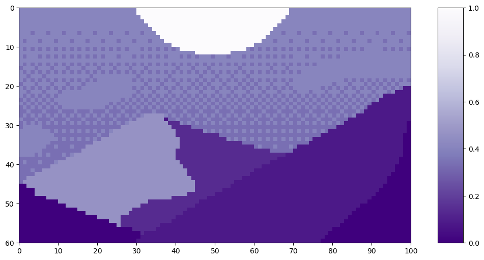
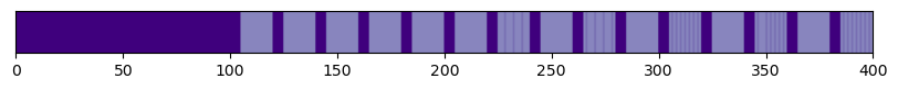
Let’s look at an example of the soft split on this pixel art Mountain at Dusk by Luis Zuno (@ansimuz)⁴. The original artwork has been cropped and converted to a single channel image. This means that each pixel has a value between zero and one. Single channel images are typically displayed in grayscale; however, we’ll be displaying it in a purple color scheme because its easier to see.
This image has size H=60 and W=100. We’ll use a patch size — or equivalently kernel — of k=20. T2T-ViT sets the stride — a measure of overlap — at s=ceil(k/2) and the padding at p=ceil(k/4). For our example, that means we’ll use s=10 and p=5. The padding is all zero values, which appear as the darkest purple.
Before we can look at the patches created in the soft split, we have to know how many patches there will be. The soft splits are implemented as torch.nn.Unfold⁵ layers. To calculate how many tokens the soft split will create, we use the following formula:
where h is the original image height, w is the original image width, k is the kernel size, s is the stride size, and p is the padding size⁵. This formula assumes the kernel is square, and that the stride and padding are symmetric. Additionally, it assumes that dilation is 1.
An aside about dilation: PyTorch describes dilation as “control[ling] the spacing between the kernel points”⁵, and refers readers to the diagram here. A dilation=1 value keeps the kernel as you would expect, all pixels touching. A user in this forum suggests to think about it as “every dilation-th element is used.” In this case, every 1st element is used, meaning every element is used.
The first term in the num_tokens equation describes how many tokens are along the height, while the second term describes how many tokens are along the width. We implement this in code below:
def count_tokens(w, h, k, s, p): """ Function to count how many tokens are produced from a given soft split
Args: w (int): starting width h (int): starting height k (int): kernel size s (int): stride size p (int): padding size
Returns: new_w (int): number of tokens along the width new_h (int): number of tokens along the height total (int): total number of tokens created """
Using the dimensions in the Mountain at Dusk⁴ example:
k = 20
s = 10
p = 5
padded_H = H + 2*p
padded_W = W + 2*p
print('With padding, the image will be H =', padded_H, 'and W =', padded_W, 'pixels.n')

patches_w, patches_h, total_patches = count_tokens(w=W, h=H, k=k, s=s, p=p)
print('There will be', total_patches, 'patches as a result of the soft split;')
print(patches_h, 'along the height and', patches_w, 'along the width.')
With padding, the image will be H = 70 and W = 110 pixels.

There will be 60 patches as a result of the soft split;
6 along the height and 10 along the width.
Now, we can see how the soft split creates patches from the Mountain at Dusk⁴.
We can see how the soft split results in overlapping patches. By counting the patches as they move across the image, we can see that there are 6 patches along the height and 10 patches along the width, exactly as predicted. By flattening these patches, we see the resulting tokens. Let’s flatten the first patch as an example.
print('Each patch will make a token of length', str(k**2)+'.') print('n')
You can see the large areas of padding in the top left and bottom right of the matrix, as well as in smaller segments throughout. Now, our tokens are ready to be passed along to the next step.
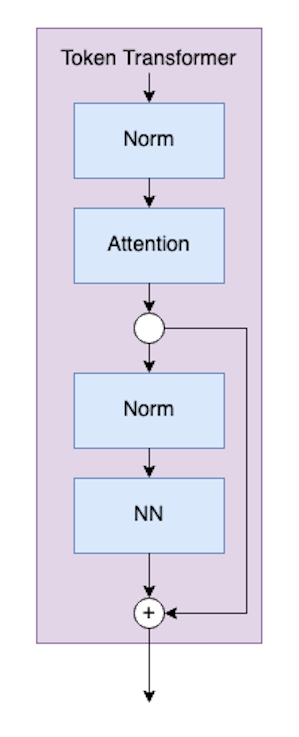
Token Transformer
The next component of the T2T module is the Token Transformer, which is represented by the purple blocks.
Token Transformer (image by author)
The code for the Token Transformer class looks like:
Args: dim (int): size of a single token chan (int): resulting size of a single token num_heads (int): number of attention heads in MSA hidden_chan_mul (float): multiplier to determine the number of hidden channels (features) in the NeuralNet module qkv_bias (bool): determines if the attention qkv layer learns an addative bias qk_scale (NoneFloat): value to scale the queries and keys by; if None, queries and keys are scaled by ``head_dim ** -0.5`` act_layer(nn.modules.activation): torch neural network layer class to use as activation in the NeuralNet module norm_layer(nn.modules.normalization): torch neural network layer class to use as normalization """
def forward(self, x): x = self.attn(self.norm1(x)) x = x + self.neuralnet(self.norm2(x)) return x
The chan, num_heads, qkv_bias, and qk_scale parameters define the Attention module components. A deep dive into attention for vistransformers is best left for another time.
The hidden_chan_mul and act_layer parameters define the Neural Network module components. The activation layer can be any torch.nn.modules.activation⁶ layer. The norm_layer can be chosen from any torch.nn.modules.normalization⁷ layer.
Let’s step through each blue block in the diagram. We’re using 7∗7=49 as our starting token size, since the fist soft split has a default kernel of 7×7.³ We’re using 64 channels because that’s also the default³. We’re using 100 tokens because it’s a nice number. We’re using a batch size of 13 because it’s prime and won’t be confused for any of the other parameters. We’re using 4 heads because it divides the channels; however, you won’t see the head dimension in the Token Transformer Module.
Input dimensions are
    batchsize: 13
    number of tokens: 100
    token size: 49
First, we pass the input through a norm layer, which does not change it’s shape. Next, it gets passed through the first Attention module, which changes the length of the tokens. Recall that a more in-depth explanation for Attention in VisTransformers can be found here.
x = TT.norm1(x)
print('After norm, dimensions arentbatchsize:', x.shape[0], 'ntnumber of tokens:', x.shape[1], 'nttoken size:', x.shape[2])
x = TT.attn(x)
print('After attention, dimensions arentbatchsize:', x.shape[0], 'ntnumber of tokens:', x.shape[1], 'nttoken size:', x.shape[2])
After norm, dimensions are
   batchsize: 13
   number of tokens: 100
   token size: 49
After attention, dimensions are
   batchsize: 13
   number of tokens: 100
   token size: 64
Now, we must save the state for a split connection layer. In the actual class definition, this is done more efficiently in one line. However, for this walk through, we do it separately.
Next, we can pass it through another norm layer and then the Neural Network module. The norm layer doesn’t change the shape of the input. The neural network is configured to also not change the shape.
The last step is the split connection, which also does not change the shape.
y = TT.norm2(x)
print('After norm, dimensions arentbatchsize:', x.shape[0], 'ntnumber of tokens:', x.shape[1], 'nttoken size:', x.shape[2])
y = TT.neuralnet(y)
print('After neural net, dimensions arentbatchsize:', x.shape[0], 'ntnumber of tokens:', x.shape[1], 'nttoken size:', x.shape[2])
y = y + x
print('After split connection, dimensions arentbatchsize:', x.shape[0], 'ntnumber of tokens:', x.shape[1], 'nttoken size:', x.shape[2])
After norm, dimensions are
   batchsize: 13
   number of tokens: 100
   token size: 64
After neural net, dimensions are
   batchsize: 13
   number of tokens: 100
   token size: 64
After split connection, dimensions are
   batchsize: 13
   number of tokens: 100
   token size: 64
That’s all for the Token Transformer Module.
Neural Network Module
The neural network (NN) module is a sub-component of the token transformer module. The neural network module is very simple, consisting of a fully-connected layer, an activation layer, and another fully-connected layer. The activation layer can be any torch.nn.modules.activation⁶ layer, which is passed as input to the module. The NN module can be configured to change the shape of an input, or to maintain the same shape. We’re not going to step through this code, as NNs are common in machine learning, and not the focus of this article. However, the code for the NN module is presented below.
Args: in_chan (int): number of channels (features) at input hidden_chan (NoneFloat): number of channels (features) in the hidden layer; if None, number of channels in hidden layer is the same as the number of input channels out_chan (NoneFloat): number of channels (features) at output; if None, number of output channels is same as the number of input channels act_layer(nn.modules.activation): torch neural network layer class to use as activation """
super().__init__()
## Define Number of Channels hidden_chan = hidden_chan or in_chan out_chan = out_chan or in_chan
def forward(self, x): x = self.fc1(x) x = self.act(x) x = self.fc2(x) return x
Image Reconstruction
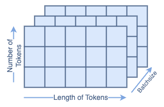
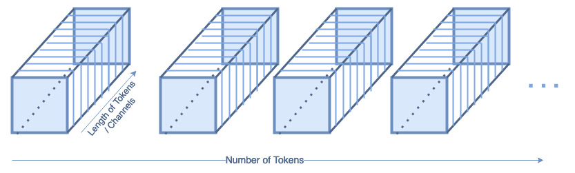
The image reconstruction layers are also shown as blue blocks inside the T2T diagram. The shape of the input to the reconstruction layers looks like (batch, num_tokens, tokensize=channels). If we look at just one batch, that looks like this:
Single Batch of Tokens (image by author)
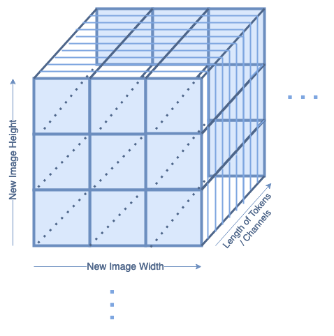
The reconstruction layers reshape the tokens into a 2D image again, which looks like this:
Reconstructed Image (image by author)
In each batch, there will be tokensize = channel number of reconstructed images. This is handled in the same way as if the image was in color, and had three color channels.
The code for reconstruction isn’t wrapped in it’s own function. However, an example is shown below:
Args: img_size (tuple[int, int, int]): size of input (channels, height, width) token_chan (int): number of token channels inside the TokenTransformers token_len (int): desired length of an output token """
## Soft Split 2 x = self.soft_split2(x).transpose(1, 2)
## Project Tokens to desired length x = self.project(x)
return x
Let’s walk through the forward pass. Since we already examined the components in more depth, this section will treat them as black boxes: we’ll just be looking at the input and outputs.
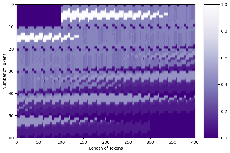
We’ll define an input to the network of shape 1x400x100 to represent a grayscale (one channel) rectangular image. We’re using 64 channels and 768 token length because those are the default values³. We’re using a batch size of 13 because it’s prime and won’t be confused for any of the other parameters.
# Define an Input H = 400 W = 100 channels = 64 batch = 13 x = torch.rand(batch, 1, H, W) print('Input dimensions arentbatchsize:', x.shape[0], 'ntnumber of input channels:', x.shape[1], 'ntimage size:', (x.shape[2], x.shape[3]))
Input dimensions are
   batchsize: 13
   number of input channels: 1
   image size: (400, 100)
The input image is first passed through a soft split layer with kernel = 7, stride = 4, and padding = 2. The length of the tokens will be the kernel size (7∗7=49) times the number of channels (= 1 for grayscale input). We can use the count_tokens function to calculate how many tokens there should be after the soft split.
# Count Tokens
k = 7
s = 4
p = 2
_, _, T = count_tokens(w=W, h=H, k=k, s=s, p=p)
print('There should be', T, 'tokens after the soft split.')
print('They should be of length', k, '*', k, '* 1 =', k*k*1)

# Perform the Soft Split
x = T2T.soft_split0(x)
print('Dimensions after soft split arentbatchsize:', x.shape[0], 'nttoken length:', x.shape[1], 'ntnumber of tokens:', x.shape[2])
x = x.transpose(1, 2)
There should be 2500 tokens after the soft split.
They should be of length 7 * 7 * 1 = 49
Dimensions after soft split are
   batchsize: 13
   token length: 49
   number of tokens: 2500
Next, we pass through the first Token Transformer. This does not impact the batch size or number of tokens, but it changes the length of the tokens to be channels = 64.
x = T2T.transformer1(x)
print('Dimensions after transformer arentbatchsize:', x.shape[0], 'ntnumber of tokens:', x.shape[1], 'nttoken length:', x.shape[2])
Dimensions after transformer are
   batchsize: 13
   number of tokens: 2500
   token length: 64
Now, we reconstruct the tokens back into a 2D image. The count_tokens function again can tell us the shape of the new image. It will have 64 channels, the same as the length of the tokens coming out of the Token Transformer.
W, H, _ = count_tokens(w=W, h=H, k=7, s=4, p=2)
print('The reconstructed image should have shape', (H, W))

x = x.transpose(1,2).reshape(B, T2T.token_chan, H, W)
print('Dimensions of reconstructed image arentbatchsize:', x.shape[0], 'ntnumber of input channels:', x.shape[1], 'ntimage size:', (x.shape[2], x.shape[3]))
The reconstructed image should have shape (100, 25)
Dimensions of reconstructed image are
   batchsize: 13
   number of input channels: 64
   image size: (100, 25)
Now that we have a 2D image again, we go back to the soft split! The next code block goes through the second soft split, the second Token Transformer, and the second image reconstruction.
# Soft Split
k = 3
s = 2
p = 1
_, _, T = count_tokens(w=W, h=H, k=k, s=s, p=p)
print('There should be', T, 'tokens after the soft split.')
print('They should be of length', k, '*', k, '*', T2T.token_chan, '=', k*k*T2T.token_chan)
x = T2T.soft_split1(x)
print('Dimensions after soft split arentbatchsize:', x.shape[0], 'nttoken length:', x.shape[1], 'ntnumber of tokens:', x.shape[2])
x = x.transpose(1, 2)

# Token Transformer
x = T2T.transformer2(x)
print('Dimensions after transformer arentbatchsize:', x.shape[0], 'ntnumber of tokens:', x.shape[1], 'nttoken length:', x.shape[2])

# Reconstruction
W, H, _ = count_tokens(w=W, h=H, k=k, s=s, p=p)
print('The reconstructed image should have shape', (H, W))
x = x.transpose(1,2).reshape(batch, T2T.token_chan, H, W)
print('Dimensions of reconstructed image arentbatchsize:', x.shape[0], 'ntnumber of input channels:', x.shape[1], 'ntimage size:', (x.shape[2], x.shape[3]))
There should be 650 tokens after the soft split.
They should be of length 3 * 3 * 64 = 576
Dimensions after soft split are
   batchsize: 13
   token length: 576
   number of tokens: 650
Dimensions after transformer are
   batchsize: 13
   number of tokens: 650
   token length: 64
The reconstructed image should have shape (50, 13)
Dimensions of reconstructed image are
   batchsize: 13
   number of input channels: 64
   image size: (50, 13)
From this reconstructed image, we go through a final soft split. Recall that the output of the T2T module should be a list of tokens.
# Soft Split
_, _, T = count_tokens(w=W, h=H, k=3, s=2, p=1)
print('There should be', T, 'tokens after the soft split.')
print('They should be of length 3*3*64=', 3*3*64)
x = T2T.soft_split2(x)
print('Dimensions after soft split arentbatchsize:', x.shape[0], 'nttoken length:', x.shape[1], 'ntnumber of tokens:', x.shape[2])
x = x.transpose(1, 2)
There should be 175 tokens after the soft split.
They should be of length 3 * 3 * 64 = 576
Dimensions after soft split are
   batchsize: 13
   token length: 576
   number of tokens: 175
The last layer in the T2T module is a linear layer to project the tokens to the desired output size. We specified that as token_len=768.
x = T2T.project(x)
print('Output dimensions arentbatchsize:', x.shape[0], 'ntnumber of tokens:', x.shape[1], 'nttoken length:', x.shape[2])
Output dimensions are
   batchsize: 13
   number of tokens: 175
   token length: 768
And that concludes the T2T Module!
ViT Backbone
From the T2T module, the tokens proceed through a ViT backbone. This is identical to the backbone of the ViT model described in [2]. The Vision Transformers article does an in-depth walk through of the ViT model and the ViT backbone. The code is reproduced below, but we won’t do a walk-through. Check that out here and then come back!
""" VisTransformer Backbone Args: preds (int): number of predictions to output token_len (int): length of a token num_heads(int): number of attention heads in MSA Encoding_hidden_chan_mul (float): multiplier to determine the number of hidden channels (features) in the NeuralNet component of the Encoding Module depth (int): number of encoding blocks in the model qkv_bias (bool): determines if the qkv layer learns an addative bias qk_scale (NoneFloat): value to scale the queries and keys by; if None, queries and keys are scaled by ``head_dim ** -0.5`` act_layer(nn.modules.activation): torch neural network layer class to use as activation norm_layer(nn.modules.normalization): torch neural network layer class to use as normalization """
## Make the class token sampled from a truncated normal distrobution timm.layers.trunc_normal_(self.cls_token, std=.02)
def forward(self, x): ## Assumes x is already tokenized
## Get Batch Size B = x.shape[0] ## Concatenate Class Token x = torch.cat((self.cls_token.expand(B, -1, -1), x), dim=1) ## Add Positional Embedding x = x + self.pos_embed ## Run Through Encoding Blocks for blk in self.blocks: x = blk(x) ## Take Norm x = self.norm(x) ## Make Prediction on Class Token x = self.head(x[:, 0]) return x
Complete Code
To create the complete T2T-ViT module, we use the T2T module and the ViT Backbone.
Args: img_size (tuple[int, int, int]): size of input (channels, height, width) softsplit_kernels (tuple[int int, int]): size of the square kernel for each of the soft split layers, sequentially preds (int): number of predictions to output token_len (int): desired length of an output token token_chan (int): number of token channels inside the TokenTransformers num_heads(int): number of attention heads in MSA (only works if =1) T2T_hidden_chan_mul (float): multiplier to determine the number of hidden channels (features) in the NeuralNet component of the Tokens-to-Token (T2T) Module Encoding_hidden_chan_mul (float): multiplier to determine the number of hidden channels (features) in the NeuralNet component of the Encoding Module depth (int): number of encoding blocks in the model qkv_bias (bool): determines if the qkv layer learns an addative bias qk_scale (NoneFloat): value to scale the queries and keys by; if None, queries and keys are scaled by ``head_dim ** -0.5`` act_layer(nn.modules.activation): torch neural network layer class to use as activation norm_layer(nn.modules.normalization): torch neural network layer class to use as normalization """
## Initialize the Weights self.apply(self._init_weights)
def _init_weights(self, m): """ Initialize the weights of the linear layers & the layernorms """ ## For Linear Layers if isinstance(m, nn.Linear): ## Weights are initialized from a truncated normal distrobution timmm.trunc_normal_(m.weight, std=.02) if isinstance(m, nn.Linear) and m.bias is not None: ## If bias is present, bias is initialized at zero nn.init.constant_(m.bias, 0) ## For Layernorm Layers elif isinstance(m, nn.LayerNorm): ## Weights are initialized at one nn.init.constant_(m.weight, 1.0) ## Bias is initialized at zero nn.init.constant_(m.bias, 0)
@torch.jit.ignore ##Tell pytorch to not compile as TorchScript def no_weight_decay(self): """ Used in Optimizer to ignore weight decay in the class token """ return {'cls_token'}
def forward(self, x): x = self.tokens_to_token(x) x = self.vit_backbone(x) return x
In the T2T-ViT Model, the img_size and softsplit_kernels parameters define the soft splits in the T2T module. The num_heads, token_chan, qkv_bias, and qk_scale parameters define the Attention modules within the Token Transformer modules, which are themselves within the T2T module. The T2T_hidden_chan_mul and act_layer define the NN module within the Token Transformer module. The token_len defines the linear layers in the T2T module. The norm_layer defines the norms.
Similarly, the num_heads, token_len, qkv_bias, and qk_scale parameters define the Attention modules within the Encoding Blocks, which are themselves within the ViT Backbone. The Encoding_hidden_chan_mul and act_layer define the NN module within the Encoding Blocks. The depth parameter defines how many Encoding Blocks are in the ViT Backbone. The norm_layer defines the norms. The preds parameter defines the prediction head in the ViT Backbone.
The act_layer can be any torch.nn.modules.activation⁶ layer, and the norm_layer can be any torch.nn.modules.normalization⁷ layer.
The _init_weights method sets custom initial weights for model training. This method could be deleted to initiate all learned weights and biases randomly. As implemented, the weights of linear layers are initialized as a truncated normal distribution; the biases of linear layers are initialized as zero; the weights of normalization layers are initialized as one; the biases of normalization layers are initialized as zero.
Conclusion
Now, you can go forth and train T2T-ViT models with a deep understanding of their mechanics! The code in this article an be found in the GitHub repository for this series. The code from the T2T-ViT paper³ can be found here. Happy transforming!
This article was approved for release by Los Alamos National Laboratory as LA-UR-23–33876. The associated code was approved for a BSD-3 open source license under O#4693.
We use cookies on our website to give you the most relevant experience by remembering your preferences and repeat visits. By clicking “Accept”, you consent to the use of ALL the cookies.
This website uses cookies to improve your experience while you navigate through the website. Out of these, the cookies that are categorized as necessary are stored on your browser as they are essential for the working of basic functionalities of the website. We also use third-party cookies that help us analyze and understand how you use this website. These cookies will be stored in your browser only with your consent. You also have the option to opt-out of these cookies. But opting out of some of these cookies may affect your browsing experience.
Necessary cookies are absolutely essential for the website to function properly. These cookies ensure basic functionalities and security features of the website, anonymously.
Cookie
Duration
Description
cookielawinfo-checkbox-analytics
11 months
This cookie is set by GDPR Cookie Consent plugin. The cookie is used to store the user consent for the cookies in the category "Analytics".
cookielawinfo-checkbox-functional
11 months
The cookie is set by GDPR cookie consent to record the user consent for the cookies in the category "Functional".
cookielawinfo-checkbox-necessary
11 months
This cookie is set by GDPR Cookie Consent plugin. The cookies is used to store the user consent for the cookies in the category "Necessary".
cookielawinfo-checkbox-others
11 months
This cookie is set by GDPR Cookie Consent plugin. The cookie is used to store the user consent for the cookies in the category "Other.
cookielawinfo-checkbox-performance
11 months
This cookie is set by GDPR Cookie Consent plugin. The cookie is used to store the user consent for the cookies in the category "Performance".
viewed_cookie_policy
11 months
The cookie is set by the GDPR Cookie Consent plugin and is used to store whether or not user has consented to the use of cookies. It does not store any personal data.
Functional cookies help to perform certain functionalities like sharing the content of the website on social media platforms, collect feedbacks, and other third-party features.
Performance cookies are used to understand and analyze the key performance indexes of the website which helps in delivering a better user experience for the visitors.
Analytical cookies are used to understand how visitors interact with the website. These cookies help provide information on metrics the number of visitors, bounce rate, traffic source, etc.
Advertisement cookies are used to provide visitors with relevant ads and marketing campaigns. These cookies track visitors across websites and collect information to provide customized ads.