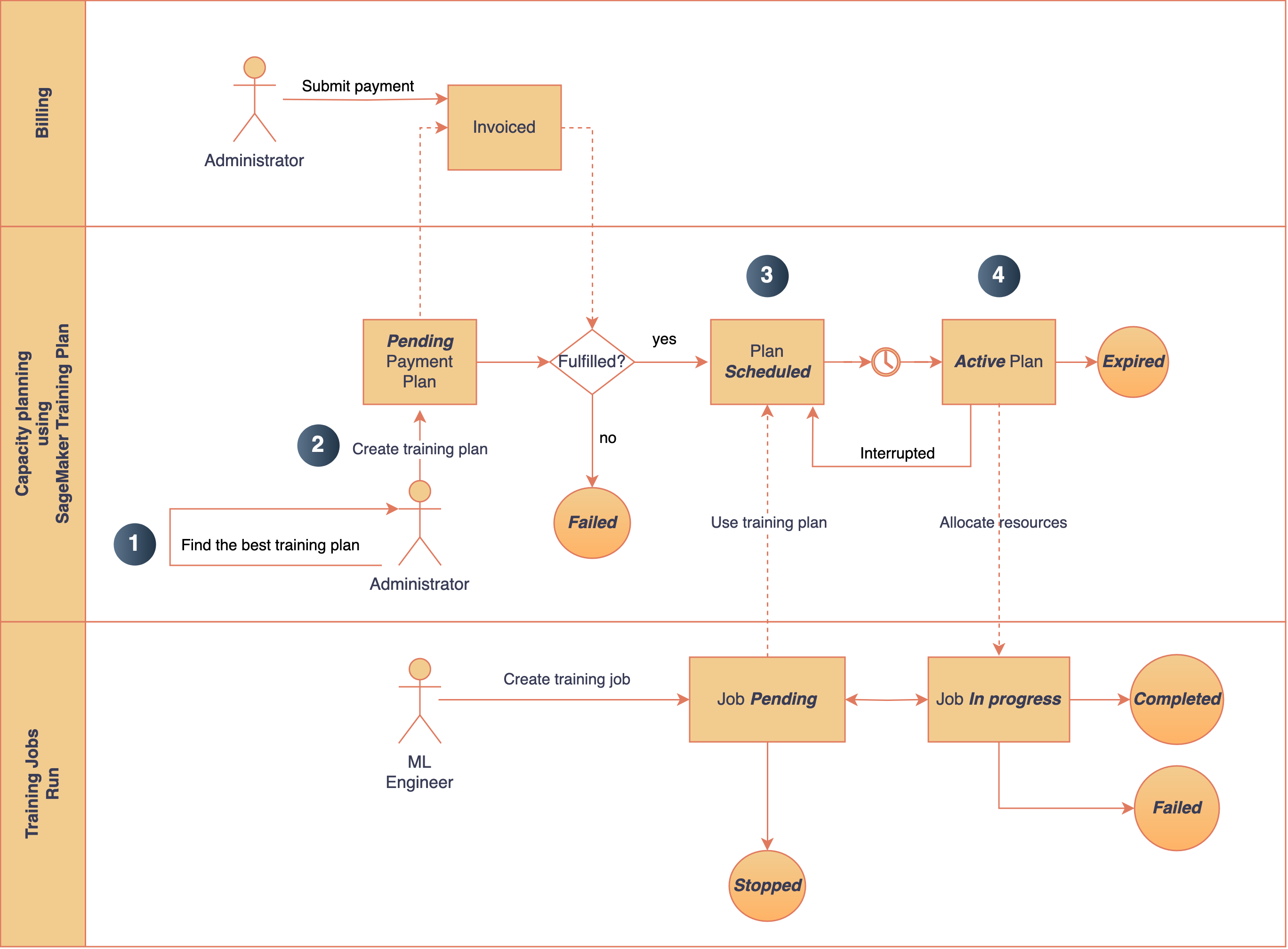
In this post, we demonstrate how you can use Amazon SageMaker HyperPod training plans, to bring down your training cluster procurement wait time. We guide you through a step-by-step implementation on how you can use the (AWS CLI) or the AWS Management Console to find, review, and create optimal training plans for your specific compute and timeline needs. We further guide you through using the training plan to submit SageMaker training jobs or create SageMaker HyperPod clusters.
With January just around the corner, we’re about to enter prime career-moves season: that exciting time of the year when many data and machine learning professionals assess their career growth and explore new opportunities, and newcomers to the field plan the next steps towards landing their first job. (It’s also when companies tend to ramp up their hiring after the end-of-year lull.)
All this energy often comes with nontrivial amounts of uncertainty, stress, and the occasional moment of self-doubt. To help you calmly chart your own path and avoid unnecessary second-guessing (of yourself as well as of hiring teams, colleagues, and others), we put together a special edition of the Variable focused on career transitions for both new and current practitioners.
We never miss a chance to celebrate data scientists’ diverse professional and academic backgrounds, and the lineup of articles we’re presenting here reflects that range, too. Whether you’re thinking about a switch to management, are about to jump into your first startup job, or are in the midst of transitioning to data science from a totally different discipline, you’ll find some concrete, experience-based insights to learn from.
Rewiring My Career: How I Transitioned from Electrical Engineering to Data Engineering When your goal is to jump across discipline lines, one of the toughest challenges is learning how to translate existing skills and knowledge and make their value apparent to prospective employers. Loizos Loizou’s debut TDS article offers a detailed account of the author’s successful repositioning from a trained electrical engineer to a data engineer—a change that is far more substantive than the title alone suggests.
Why STEM Is Important for Any Data Scientist A background in the so-called hard sciences doesn’t always map directly onto data-focused job descriptions. As Radmila M. explains, however, the benefits of applying your hard-earned STEM expertise once you’ve moved on to data science are many — and can manifest themselves in unexpected moments when traditional problem-solving approaches fail to produce the desired outcome.
From Data Scientist to Data Manager: My First 3 Months Leading a Team After nearly seven years as a data scientist, Yu Dong took on a new challenge recently and stepped into a management role for the first time. In a thoughtful new post, Yu reflects on “what has changed, what I’ve enjoyed, and what’s been challenging.”
Are You Sure You Want to Become a Data Science Manager? Tackling the management-track conundrum from a different angle, Jose Parreño encourages anyone who’s considering a move away from an individual contributor role to think deeply about their motivations and goals, and to make an informed decision based on a realistic understanding of what becoming a manager actually entails.
Roadmap to Becoming a Data Scientist, Part 1: Maths For aspiring data professionals who are still years away from debating their fit for a manager role, one of the perennial pain points remains the level and amount of math they need to master in order to start their journey on the right foot. Vyacheslav Efimov provides concrete pointers on what you should learn — and how to get started.
GenAI is Reshaping Data Science Teams Setting yourself up for success doesn’t involve a fixed formula; in fields as dynamic as data science and machine learning, the very definition of your role can evolve from one month to the next. This has been especially true in the past couple of years, as generative-AI tools and LLMs have transformed core workflows across industries. Anna Via wrote a focused synthesis of the challenges and opportunities this rapid change presents, and what data teams—and individuals within them—can do to stay nimble and adapt quickly.
Why a Data Scientist with a PhD Might Kill Your Early-Stage Startup It may sound counterintuitive that arriving at a new job with advanced educational credentials can sometimes make you less effective, but that’s precisely the point Claudia Ng drives home in her latest article. While she writes with hiring managers in mind, her insights are particularly valuable for data science PhDs who can adjust their mindset accordingly, and prevent potentially mismatched expectations.
So It’s Your First Year in AI; Here’s What to Expect Congratulations: you’ve landed your dream role at a buzzy AI startup. Now what? Based on his own personal experiences, Michael Zakhary seeks to demystify what the job might entail and to “offer a glimpse into the daily life of an ML engineer — whether you’re working in a small, agile team or part of a larger, more structured organization.”
Thank you for supporting the work of our authors! As we mentioned above, we love publishing articles from new authors, so if you’ve recently written an interesting project walkthrough, tutorial, or theoretical reflection on any of our core topics, don’t hesitate to share it with us.
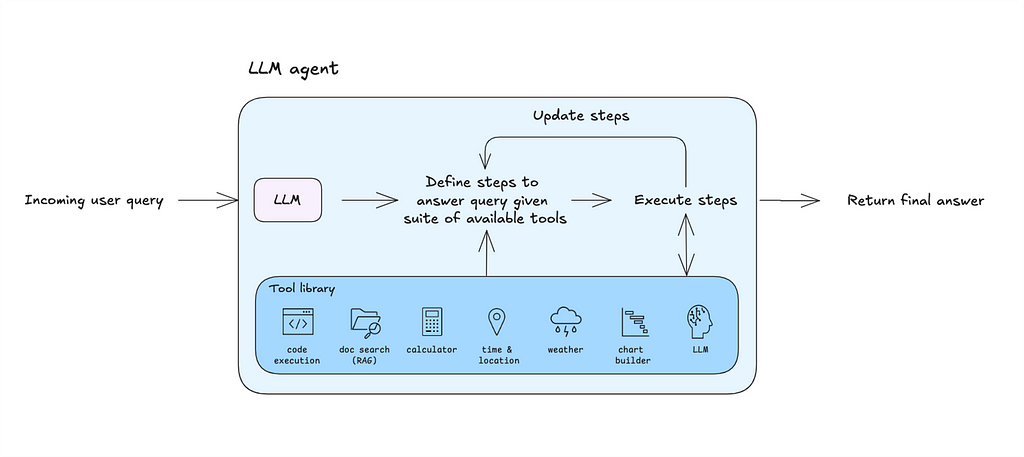
High-level Overview of an LLM Agent. (Image by author)
Why build a general-purpose agent? Because it’s an excellent tool to prototype your use cases and lays the groundwork for designing your own custom agentic architecture.
Before we dive in, let’s quickly introduce LLM agents. Feel free to skip ahead.
What is an LLM agent?
An LLM agent is a program whose execution logic is controlled by its underlying model.
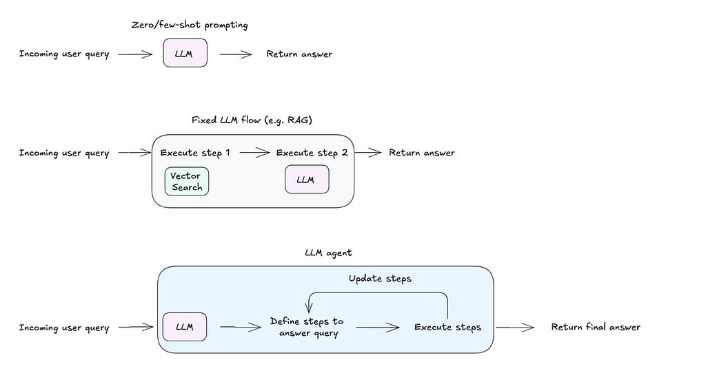
From Standalone LLMs to Agentic Systems. (Image by author)
What sets an LLM agent apart from approaches like few-shot prompting or fixed workflows is its ability to define and adapt the steps required to execute a user’s query. Given access to a set of tools (like code execution or web search), the agent can decide which tool to use, how to use it, and iterate on results based on the output. This adaptability enables the system to handle diverse use cases with minimal configuration.
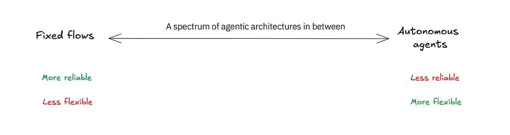
A Spectrum of Agentic Architectures. (Image by author)
Agentic architectures exist on a spectrum, ranging from the reliability of fixed workflows to the flexibility of autonomous agents. For instance, a fixed flow like Retrieval-Augmented Generation (RAG) can be enhanced with a self-reflection loop, enabling the program to iterate when the initial response falls short. Alternatively, a ReAct agent can be equipped with fixed flows as tools, offering a flexible yet structured approach. The choice of architecture ultimately depends on the use case and the desired trade-off between reliability and flexibility.
Let’s build a general-purpose LLM agent from scratch!
Step 1. Select the right LLM
Choosing the right model is critical to achieving your desired performance. There are several factors to consider, like licensing, cost, and language support. The most important consideration for building an LLM agent is the model’s performance on key tasks like coding, tool calling, and reasoning. Benchmarks to evaluate include:
Another crucial factor is the model’s context window. Agentic workflows can eat up a lot of tokens — sometimes 100K or more — a larger context window is really helpful.
In general, larger models tend to offer better performance, but smaller models that can run locally are still a solid option. With smaller models, you’ll be limited to simpler use cases and might only be able to connect your agent to one or two basic tools.
Step 2. Define the agent’s control logic (aka communication structure)
Single Agent Architecture. (Image by author)
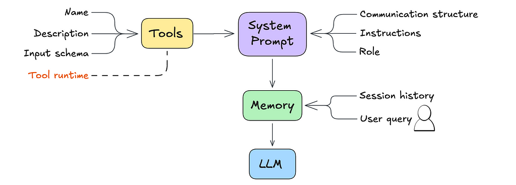
The main difference between a simple LLM and an agent comes down to the system prompt.
The system prompt, in the context of an LLM, is a set of instructions and contextual information provided to the model before it engages with user queries.
The agentic behavior expected of the LLM can be codified within the system prompt.
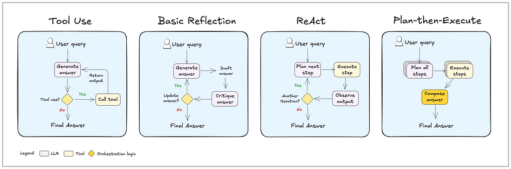
Here are some common agentic patterns, which can be customized to fit your needs:
Tool Use: The agent determines when to route queries to the appropriate tool or rely on its own knowledge.
Reflection: The agent reviews and corrects its answers before responding to the user. A reflection step can also be added to most LLM systems.
Reason-then-Act (ReAct): The agent iteratively reasons through how to solve the query, performs an action, observes the outcome, and determines whether to take another action or provide a response.
Plan-then-Execute: The agent plans upfront by breaking the task into sub-steps (if needed) and then executes each step.
The last two patterns — ReAct and Plan-then-Execute — aare often the best starting point for building a general-purpose single agent.
Overview of Common Agentic Patterns. (Image by author)
To implement these behaviors effectively, you’ll need to do some prompt engineering. You might also want to use a structured generationtechnique. This basically means shaping the LLM’s output to match a specific format or schema, so the agent’s responses stay consistent with the communication style you’re aiming for.
Example: Below is a system prompt excerpt for a ReAct style agent from the Bee Agent Framework.
# Communication structure
You communicate only in instruction lines. The format is: "Instruction: expected output". You must only use these instruction lines and must not enter empty lines or anything else between instruction lines.
You must skip the instruction lines Function Name, Function Input and Function Output if no function calling is required.

Message: User's message. You never use this instruction line.
Thought: A single-line plan of how to answer the user's message. It must be immediately followed by Final Answer.
Thought: A single-line step-by-step plan of how to answer the user's message. You can use the available functions defined above. This instruction line must be immediately followed by Function Name if one of the available functions defined above needs to be called, or by Final Answer. Do not provide the answer here.
Function Name: Name of the function. This instruction line must be immediately followed by Function Input.
Function Input: Function parameters. Empty object is a valid parameter.
Function Output: Output of the function in JSON format.
Thought: Continue your thinking process.
Final Answer: Answer the user or ask for more information or clarification. It must always be preceded by Thought.

## Examples
Message: Can you translate "How are you" into French?
Thought: The user wants to translate a text into French. I can do that.
Final Answer: Comment vas-tu?
Step 3. Define the agent’s core instructions
We tend to take for granted that LLMs come with a bunch of features right out of the box. Some of these are great, but others might not be exactly what you need. To get the performance you’re after, it’s important to spell out all the features you want — and don’t want — in the system prompt.
This could include instructions like:
Agent Name and Role: What the agent is called and what it’s meant to do.
Tone and Conciseness: How formal or casual it should sound, and how brief it should be.
When to Use Tools: Deciding when to rely on external tools versus the model’s own knowledge.
Handling Errors: What the agent should do when something goes wrong with a tool or process.
Example: Below is a snippet of the instructions section from the Bee Agent Framework.
# Instructions
User can only see the Final Answer, all answers must be provided there.
You must always use the communication structure and instructions defined above. Do not forget that Thought must be a single-line immediately followed by Final Answer.
You must always use the communication structure and instructions defined above. Do not forget that Thought must be a single-line immediately followed by either Function Name or Final Answer.
Functions must be used to retrieve factual or historical information to answer the message.
If the user suggests using a function that is not available, answer that the function is not available. You can suggest alternatives if appropriate.
When the message is unclear or you need more information from the user, ask in Final Answer.

# Your capabilities
Prefer to use these capabilities over functions.
- You understand these languages: English, Spanish, French.
- You can translate and summarize, even long documents.

# Notes
- If you don't know the answer, say that you don't know.
- The current time and date in ISO format can be found in the last message.
- When answering the user, use friendly formats for time and date.
- Use markdown syntax for formatting code snippets, links, JSON, tables, images, files.
- Sometimes, things don't go as planned. Functions may not provide useful information on the first few tries. You should always try a few different approaches before declaring the problem unsolvable.
- When the function doesn't give you what you were asking for, you must either use another function or a different function input.
  - When using search engines, you try different formulations of the query, possibly even in a different language.
- You cannot do complex calculations, computations, or data manipulations without using functions.m
Step 4. Define and optimize your core tools
Tools are what give your agents their superpowers. With a narrow set of well-defined tools, you can achieve broad functionality. Key tools to include are code execution, web search, file reading, and data analysis.
For each tool, you’ll need to define the following and include it as part of the system prompt:
Tool Name: A unique, descriptive name for the capability.
Tool Description: A clear explanation of what the tool does and when to use it. This helps the agent determine when to pick the right tool.
Tool Input Schema: A schema that outlines required and optional parameters, their types, and any constraints. The agent uses this to fill in the inputs it needs based on the user’s query..
A pointer to where/how to run the tool.
Example: Below is an excerpt of an Arxiv tool implementation from Langchain Community.
class ArxivInput(BaseModel): """Input for the Arxiv tool."""
query: str = Field(description="search query to look up")
class ArxivQueryRun(BaseTool): # type: ignore[override, override] """Tool that searches the Arxiv API."""
name: str = "arxiv" description: str = ( "A wrapper around Arxiv.org " "Useful for when you need to answer questions about Physics, Mathematics, " "Computer Science, Quantitative Biology, Quantitative Finance, Statistics, " "Electrical Engineering, and Economics " "from scientific articles on arxiv.org. " "Input should be a search query." ) api_wrapper: ArxivAPIWrapper = Field(default_factory=ArxivAPIWrapper) # type: ignore[arg-type] args_schema: Type[BaseModel] = ArxivInput
In certain cases, you’ll need to optimize tools to get the performance you’re looking for. This might involve tweaking the tool name or description with some prompt engineering, setting up advanced configurations to handle common errors, or filtering the tool’s output.
Step 5. Decide on a memory handling strategy
LLMs are limited by their context window — the number of tokens they can “remember” at a time. This memory can fill up fast with things like past interactions in multi-turn conversations, lengthy tool outputs, or extra context the agent is grounded on. That’s why having a solid memory handling strategy is crucial.
Memory, in the context of an agent, refers to the system’s capability to store, recall, and utilize information from past interactions. This enables the agent to maintain context over time, improve its responses based on previous exchanges, and provide a more personalized experience.
Common Memory Handling Strategies:
Sliding Memory: Keep the last k conversation turns in memory and drop the older ones.
Token Memory: Keep the last n tokens and forget the rest.
Summarized Memory: Use the LLM to summarize the conversation at each turn and drop the individual messages.
Additionally, you can also have an LLM detect key moments to store in long-term memory. This allows the agent to “remember” important facts about the user, making the experience even more personalized.
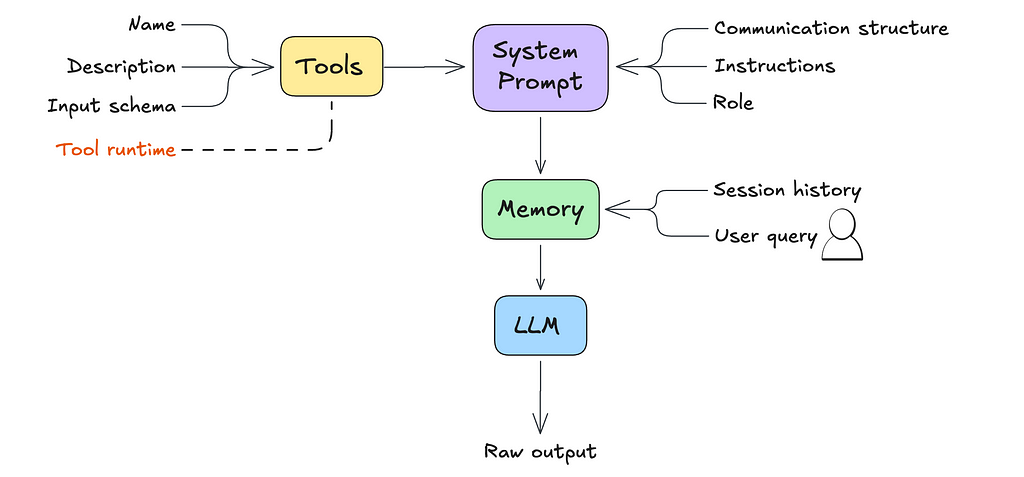
The five steps we’ve covered so far lay the foundation for setting up an agent. But what happens if we run a user query through our LLM at this stage?
Answer: you get a raw text output. (Image by author)
Here’s an example of what that might look like:
User Message: Extract key insighs from this dataset
Files: bill-of-materials.csv
Thought: First, I need to inspect the columns of the dataset and provide basic data statistics.
Function Name: Python
Function Input: {"language":"python","code":"import pandas as pdnndataset = pd.read_csv('bill-of-materials.csv')nnprint(dataset.columns)nprint(dataset.describe())","inputFiles":["bill-of-materials.csv"]}
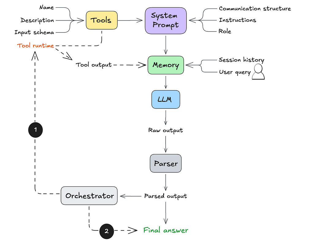
At this point, the agent produces raw text output. So how do we get it to actually execute the next step? That’s where parsing and orchestration come in.
Step 6. Parse the agent’s raw output
A parser is a function that converts raw data into a format your application can understand and work with (like an object with properties)
For the agent we’re building, the parser needs to recognize the communication structure we defined in Step 2 and return a structured output, like JSON. This makes it easier for the application to process and execute the agent’s next steps.
Note: some model providers like OpenAI, can return parsable outputs by default. For other models, especially open-source ones, this would need to be configured.
Step 7. Orchestrate the agent’s next step
The final step is setting up the orchestration logic. This determines what happens after the LLM outputs a result. Depending on the output, you’ll either:
Execute a tool call, or
Return an answer — either the final response to the user’s query or a follow-up request for more information.
Extended single agent architecture. (Image by author)
If a tool call is triggered, the tool’s output is sent back to the LLM (as part of its working memory). The LLM would then determine what to do with this new information: either performan another tool call or return an answer to the user.
Here’s an example of how this orchestration logic might look in code:
def orchestrator(llm_agent, llm_output, tools, user_query):
    """
    Orchestrates the response based on LLM output and iterates if necessary.

    Parameters:
    - llm_agent (callable): The LLM agent function for processing tool outputs.
    - llm_output (dict): Initial output from the LLM, specifying the next action.
    - tools (dict): Dictionary of available tools with their execution methods.
    - user_query (str): The original user query.

    Returns:
    - str: The final response to the user.
    """
    while True:
        action = llm_output.get("action")

        if action == "tool_call":
            # Extract tool name and parameters
            tool_name = llm_output.get("tool_name")
            tool_params = llm_output.get("tool_params", {})

            if tool_name in tools:
                try:
                    # Execute the tool
                    tool_result = tools[tool_name](**tool_params)
                    # Send tool output back to the LLM agent for further processing
                    llm_output = llm_agent({"tool_output": tool_result})
                except Exception as e:
                    return f"Error executing tool '{tool_name}': {str(e)}"
            else:
                return f"Error: Tool '{tool_name}' not found."

        elif action == "return_answer":
            # Return the final answer to the user
            return llm_output.get("answer", "No answer provided.")

        else:
            return "Error: Unrecognized action type from LLM output."
And voilà! You now have a system capable of handling a wide variety of use cases — from competitive analysis and advanced research to automating complex workflows.
Where do multi-agent systems come in?
While this generation of LLMs is incredibly powerful, they have a key limitation: they struggle with information overload. Too much context or too many tools can overwhelm the model, leading to performance issues. A general-purpose single agent will eventually hit this ceiling, especially since agents are notoriously token-hungry.
For certain use cases, a multi-agent setup might make more sense. By dividing responsibilities across multiple agents, you can avoid overloading the context of a single LLM agent and improve overall efficiency.
That said, a general-purpose single-agent setup is a fantastic starting point for prototyping. It can help you quickly test your use case and identify where things start to break down. Through this process, you can:
Understand which parts of the task truly benefit from an agentic approach.
Identify components that can be spun off as standalone processes in a larger workflow.
Starting with a single agent gives you valuable insights to refine your approach as you scale to more complex systems.
What is the best way to get started?
Ready to dive in and start building? Using a framework can be a great way to quickly test and iterate on your agent configuration.
This article begins a series for anyone who finds matrix algebra overwhelming. My goal is to turn what you’re afraid of into what you’re fascinated by. You’ll find it especially helpful if you want to understand machine learning concepts and methods.
Table of contents:
Introduction
Prerequisites
Matrix-vector multiplication
Transposition
Composition of transformations
Inverse transformation
Non-invertible transformations
Determinant
Non-square matrices
Inverse and Transpose: similarities and differences
Translation by a vector
Final words
1. Introduction
You’ve probably noticed that while it’s easy to find materials explaining matrix computation algorithms, it’s harder to find ones that teach how to interpret complex matrix expressions. I’m addressing this gap with my series, focused on the part of matrix algebra that is most commonly used by data scientists.
We’ll focus more on concrete examples rather than general formulas. I’d rather sacrifice generality for the sake of clarity and readability. I’ll often appeal to your imagination and intuition, hoping my materials will inspire you to explore more formal resources on these topics. For precise definitions and general formulas, I’d recommend you look at some good textbooks: the classic one on linear algebra¹ and the other focused on machine learning².
This part will teach you
to see a matrix as a representation of the transformation applied to data.
Let’s get started then — let me take the lead through the world of matrices.
2. Prerequisites
I’m guessing you can handle the expressions that follow.
This is the dot product written using a row vector and a column vector:
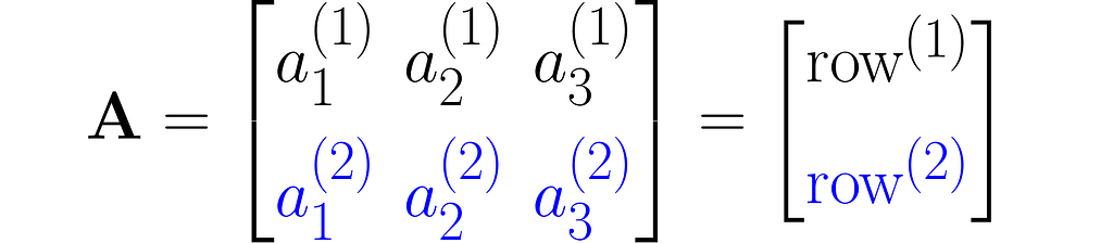
A matrix is a rectangular array of symbols arranged in rows and columns. Here is an example of a matrix with two rows and three columns:
You can view it as a sequence of columns
or a sequence of rows stacked one on top of another:
As you can see, I used superscripts for rows and subscripts for columns. In machine learning, it’s important to clearly distinguish between observations, represented as vectors, and features, which are arranged in rows.
Other interesting ways to represent this matrix are A₂ₓ₃ and A[aᵢ⁽ʲ ⁾].
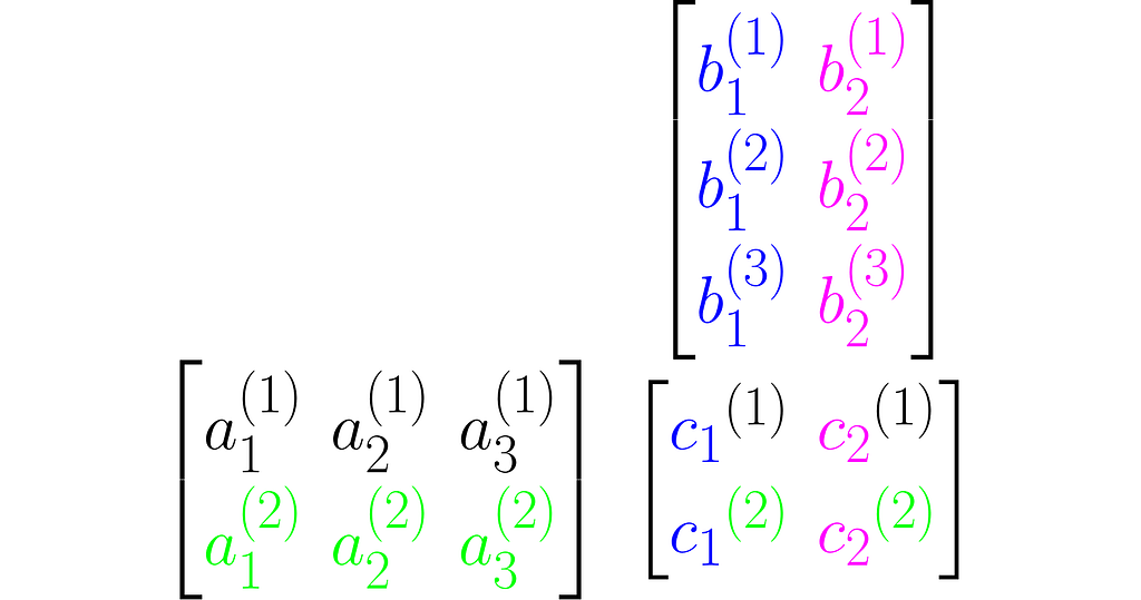
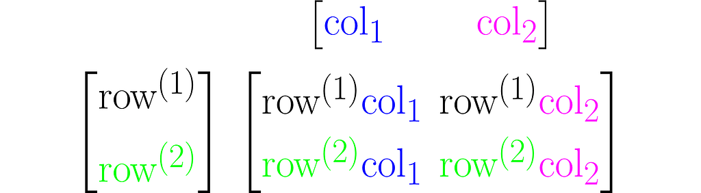
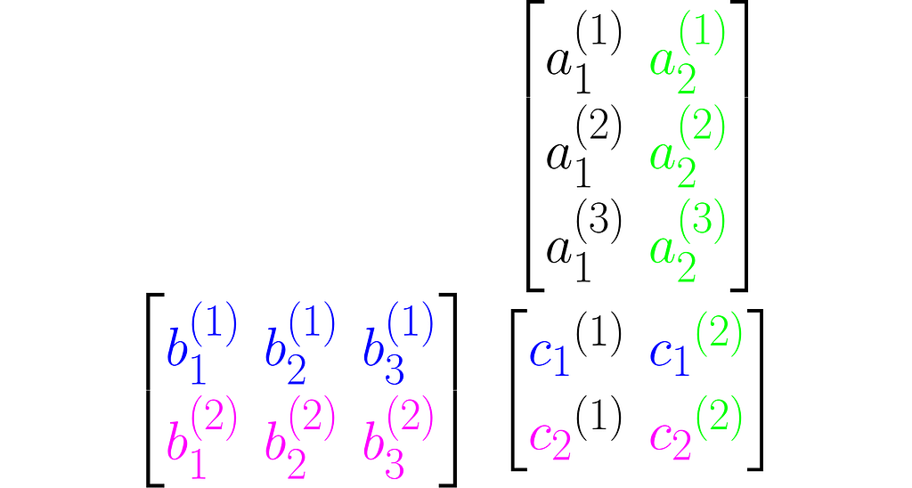
Multiplying two matrices A and B results in a third matrix C = AB containing the scalar products of each row of A with each column of B, arranged accordingly. Below is an example for C₂ₓ₂= A₂ₓ₃B₃ₓ₂.
where cᵢ⁽ʲ ⁾ is the scalar product of the i-th column of the matrix B and the j-th row of matrix A:
Note that this definition of multiplication requires the number of rows of the left matrix to match the number of columns of the right matrix. In other words, the inner dimensions of the matrices must match.
Make sure you can manually multiply matrices with arbitrary entries. You can use the following code to check the result or to practice multiplying matrices.
import numpy as np

# Matrices to be multiplied
A = [
    [ 1, 0, 2],
    [-2, 1, 1]
]

B = [
    [ 0, 3, 1],
    [-3, 1, 1],
    [-2, 2, 1]
]

# Convert to numpy array
A = np.array(A)
B = np.array(B)

# Multiply A by B (if possible)
try:
    C = A @ B
    print(f'A B = n{C}n')
except:
    print("""ValueError:
The number of rows in matrix A does not match
the number of columns in matrix B
""")

#  and in the reverse order, B by A (if possible)
try:
    D = B @ A
    print(f'B A =n{D}')
except:
    print("""ValueError:
The number of rows in matrix B does not match
the number of columns in matrix A
""")
A B =
[[-4  7]
 [-5 -3]]

B A =
[[-6  3  3]
 [-5  1 -5]
 [-6  2 -2]]
3. Matrix-vector multiplication
In this section, I will explain the effect of matrix multiplication on vectors. The vector x is multiplied by the matrix A, producing a new vector y:
This is a common operation in data science, as it enables a linear transformation of data. The use of matrices to represent linear transformations is highly advantageous, as you will soon see in the following examples.
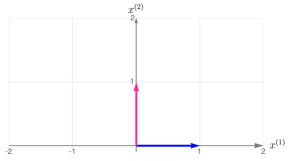
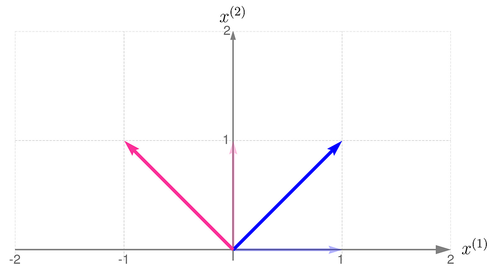
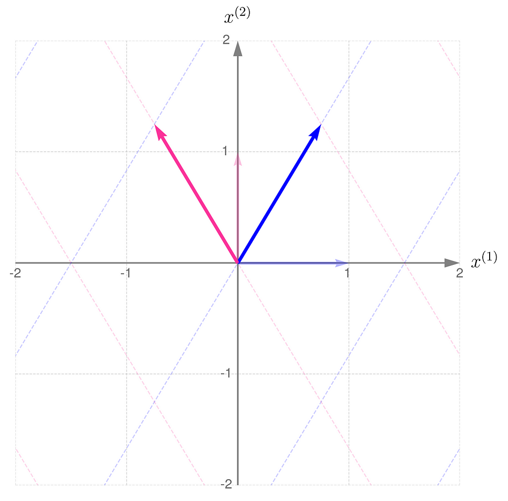
Below, you can see your grid space and your standard basis vectors: blue for the x⁽¹⁾ direction and magenta for the x⁽²⁾ direction.
Standard basis in a Grid Space
A good starting point is to work with transformations that map two-dimensional vectors x into two-dimensional vectors y in the same grid space.
Describing the desired transformation is a simple trick. You just need to say how the coordinates of the basis vectors change after the transformation and use these new coordinates as the columns of the matrix A.
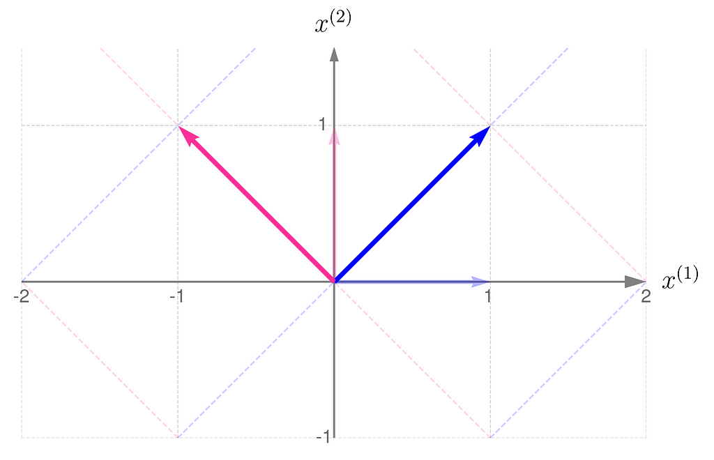
As an example, consider a linear transformation that produces the effect illustrated below. The standard basis vectors are drawn lightly, while the transformed vectors are shown more clearly.
Standard basis transformed by matrix A
From the comparison of the basis vectors before and after the transformation, you can observe that the transformation involves a 45-degree counterclockwise rotation about the origin, along with an elongation of the vectors.
This effect can be achieved using the matrix A, composed as follows:
The first column of the matrix contains the coordinates of the first basis vector after the transformation, and the second column contains those of the second basis vector.
The equation (1) then takes the form
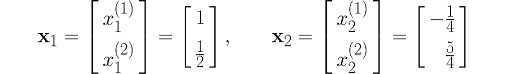
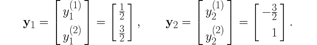
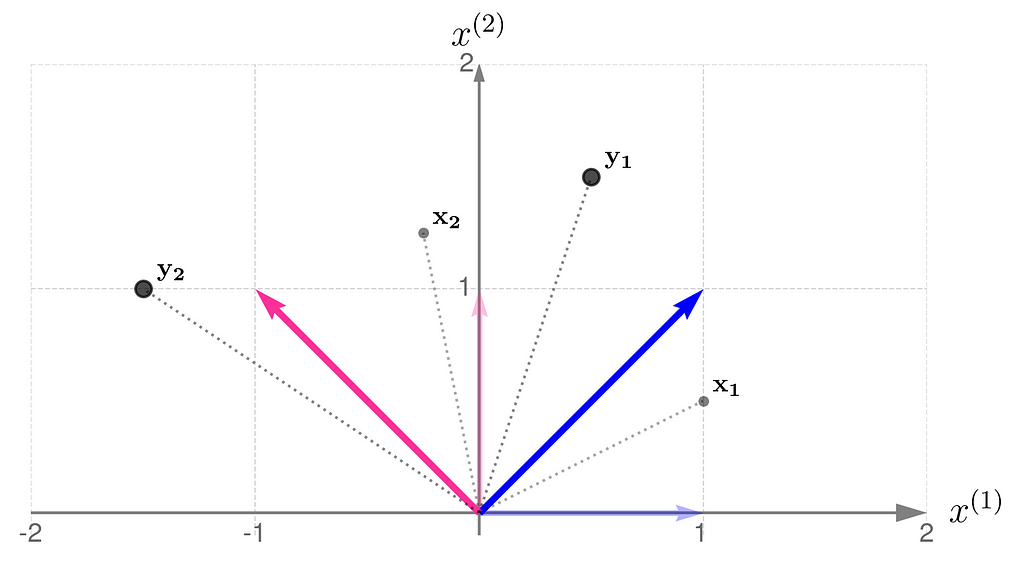
Let’s take two example points x₁and x₂ :
and transform them into the vectors y₁ and y₂ :
I encourage you to do these calculations by hand first, and then switch to using a program like this:
# Points (vectors) to be transformed using matrix A points = [ np.array([1, 1/2]), np.array([-1/4, 5/4]) ]
# Print out the transformed points (vectors) for i, x in enumerate(points): y = A @ x print(f'y_{i} = {y}')
y_0 = [0.5 1.5]
y_1 = [-1.5  1. ]
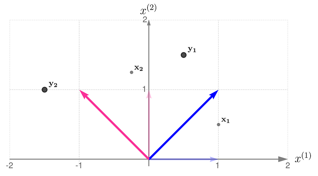
The plot below shows the results.
Points transformed by matrix A
The x points are gray and smaller, while their transformed counterparts y have black edges and are bigger. If you’d prefer to think of these points as arrowheads, here’s the corresponding illustration:
Vectors transformed by matrix A
Now you can see more clearly that the points have been rotated around the origin and pushed a little away.
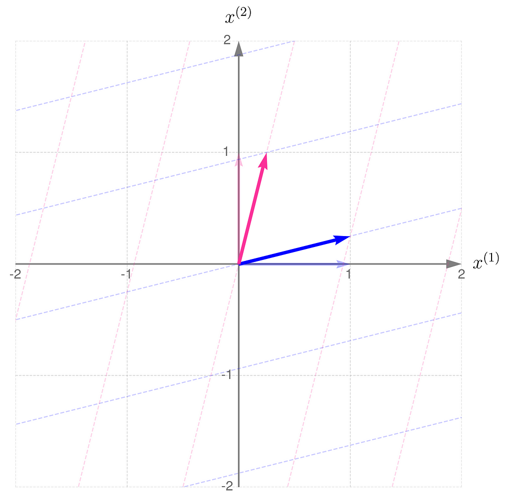
Let’s examine another matrix:
and see how the transformation
affects the points on the grid lines:
Grid lines transformed by matrix B
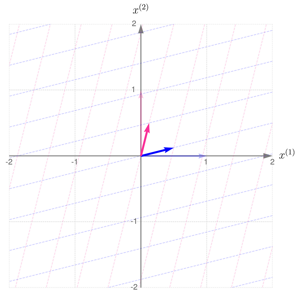
Compare the result with that obtained using B/2, which corresponds to dividing all elements of the matrix B by 2:
Grid lines transformed by matrix B/2
In general, a linear transformation:
ensures that straight lines remain straight,
keeps parallel lines parallel,
scales the distances between them by a uniform factor.
To keep things concise, I’ll use ‘transformation A‘ throughout the text instead of the full phrase ‘transformation represented by matrix A’.
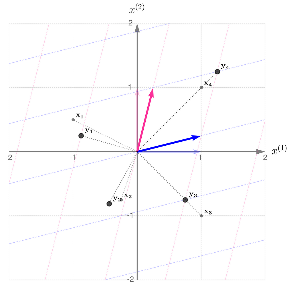
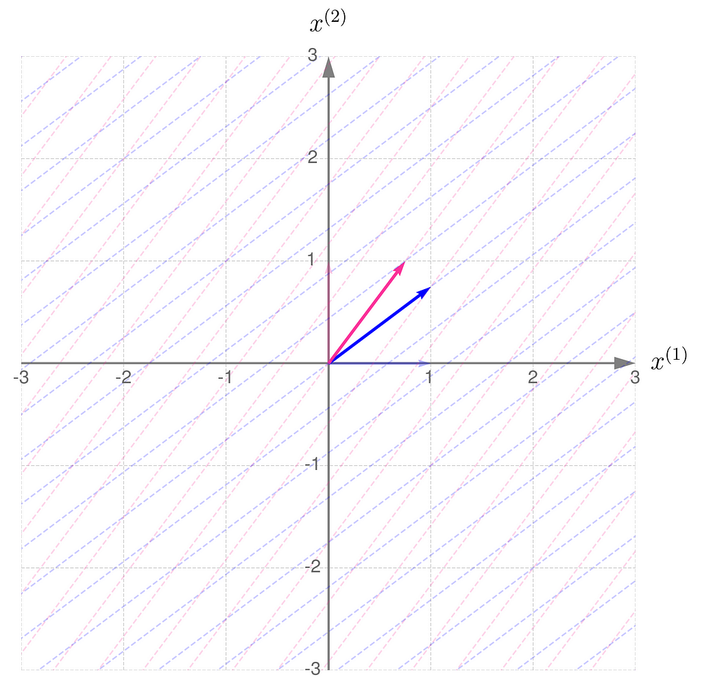
Let’s return to the matrix
and apply the transformation to a few sample points.
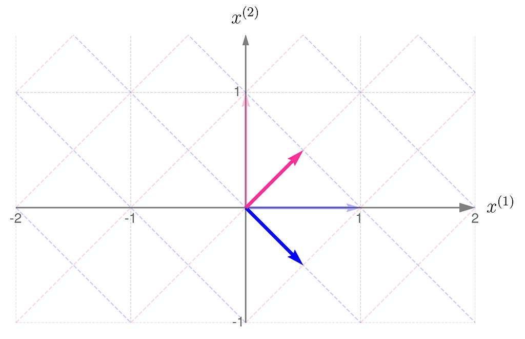
The effects of transformation B on various input vectors
Notice the following:
point x₁ has been rotated counterclockwise and brought closer to the origin,
point x₂, on the other hand, has been rotated clockwise and pushed away from the origin,
point x₃ has only been scaled down, meaning it’s moved closer to the origin while keeping its direction,
point x₄ has undergone a similar transformation, but has been scaled up.
The transformation compresses in the x⁽¹⁾-direction and stretches in the x⁽²⁾-direction. You can think of the grid lines as behaving like an accordion.
Directions such as those represented by the vectors x₃ and x₄ play an important role in machine learning, but that’s a story for another time.
For now, we can call them eigen-directions, because vectors along these directions might only be scaled by the transformation, without being rotated. Every transformation, except for rotations, has its own set of eigen-directions.
4. Transposition
Recall that the transformation matrix is constructed by stacking the transformed basis vectors in columns. Perhaps you’d like to see what happens if we swap the rows and columns afterwards (the transposition).
Let us take, for example, the matrix
where Aᵀ stands for the transposed matrix.
From a geometric perspective, the coordinates of the first new basis vector come from the first coordinates of all the old basis vectors, the second from the second coordinates, and so on.
In NumPy, it’s as simple as that:
import numpy as np

A = np.array([
    [1, -1],
    [1 , 1]
    ])

print(f'A transposed:n{A.T}')
A transposed:
[[ 1  1]
 [-1  1]]
I must disappoint you now, as I cannot provide a simple rule that expresses the relationship between the transformations A and Aᵀ in just a few words.
Instead, let me show you a property shared by both the original and transposed transformations, which will come in handy later.
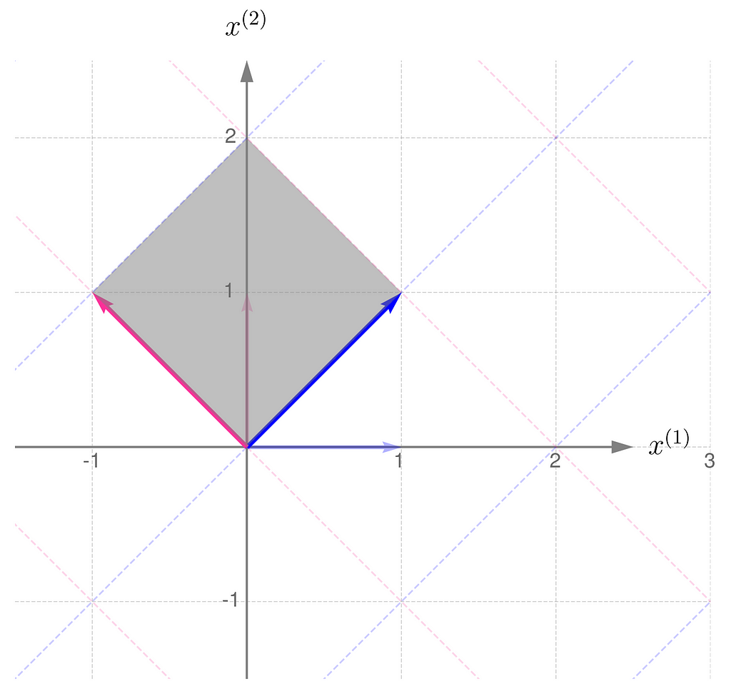
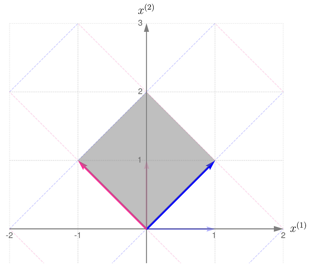
Here is the geometric interpretation of the transformation represented by the matrix A. The area shaded in gray is called the parallelogram.
Parallelogram spanned by the basis vectors transformed by matrix A
Compare this with the transformation obtained by applying the matrix Aᵀ:
Parallelogram spanned by the basis vectors transformed by matrix Aᵀ
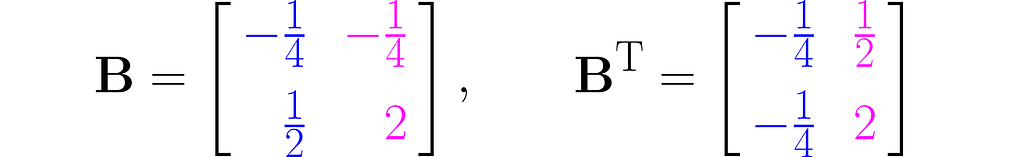
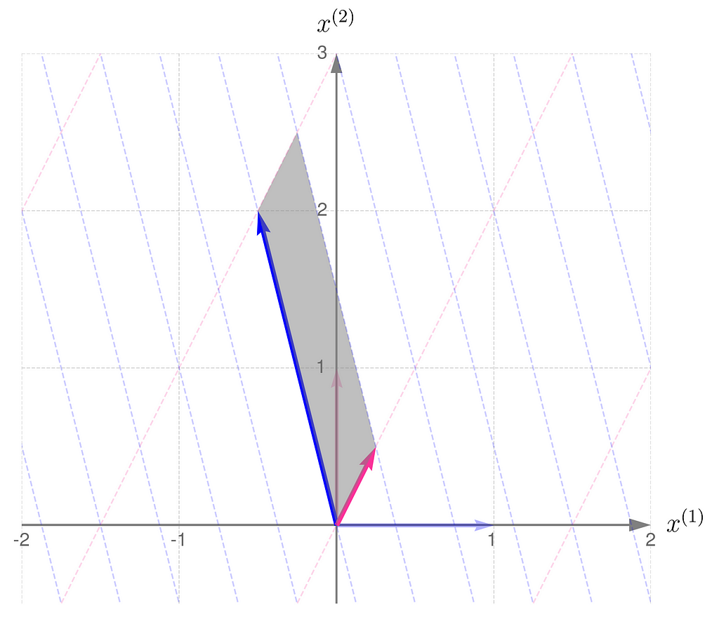
Now, let us consider another transformation that applies entirely different scales to the unit vectors:
The parallelogram associated with the matrix B is much narrower now:
Parallelogram spanned by the basis vectors transformed by matrix B
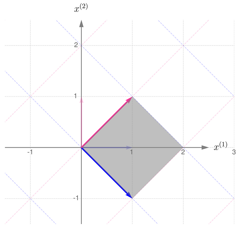
but it turns out that it is the same size as that for the matrix Bᵀ:
Parallelogram spanned by the basis vectors transformed by matrix Bᵀ
Let me put it this way: you have a set of numbers to assign to the components of your vectors. If you assign a larger number to one component, you’ll need to use smaller numbers for the others. In other words, the total length of the vectors that make up the parallelogram stays the same. I know this reasoning is a bit vague, so if you’re looking for more rigorous proofs, check the literature in the references section.
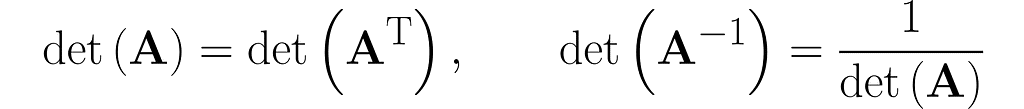
And here’s the kicker at the end of this section: the area of the parallelograms can be found by calculating the determinant of the matrix. What’s more, the determinant of the matrix and its transpose are identical.
More on the determinant in the upcoming sections.
5. Composition of transformations
You can apply a sequence of transformations — for example, start by applying A to the vector x, and then pass the result through B. This can be done by first multiplying the vector x by the matrix A, and then multiplying the result by the matrix B:
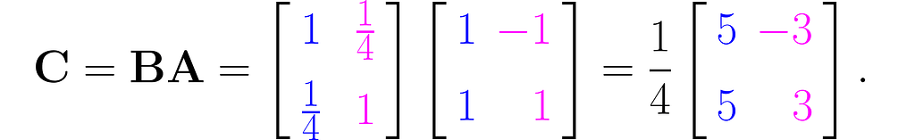
You can multiply the matrices B and A to obtain the matrix C for further use:
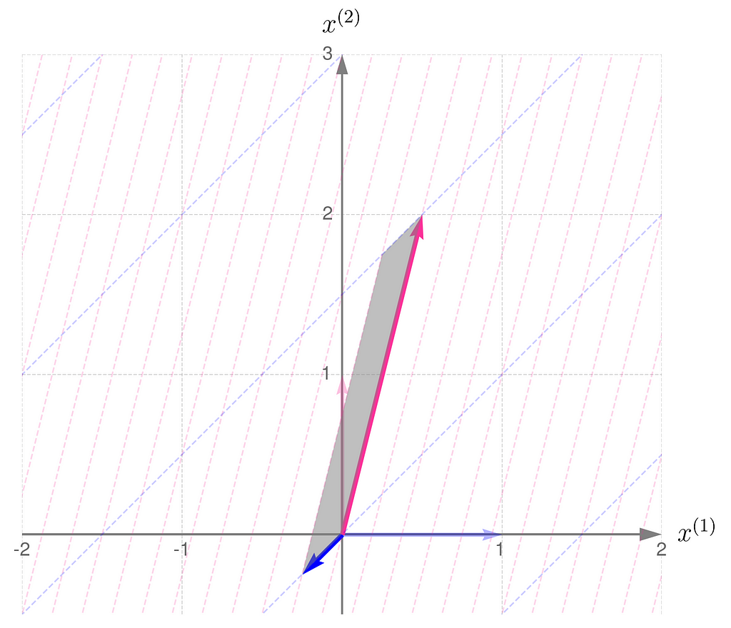
This is the effect of the transformation represented by the matrix C:
Transformation described by the composite matrix BA
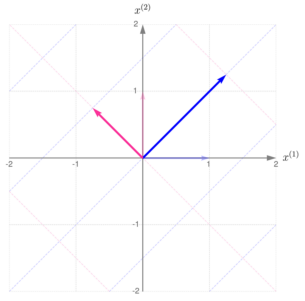
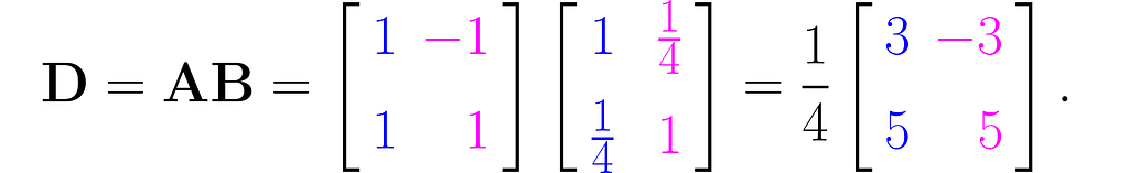
You can perform the transformations in reverse order: first apply B, then apply A:
Let D represent the sequence of multiplications performed in this order:
And this is how it affects the grid lines:
Transformation described by the composite matrix AB
So, you can see for yourself that the order of matrix multiplication matters.
There’s a cool property with the transpose of a composite transformation. Check out what happens when we multiply A by B:
and then transpose the result, which means we’ll apply (AB)ᵀ:
You can easily extend this observation to the following rule:
To finish off this section, consider the inverse problem: is it possible to recover matrices A and B given only C = AB?
This is matrix factorization, which, as you might expect, doesn’t have a unique solution. Matrix factorization is a powerful technique that can provide insight into transformations, as they may be expressed as a composition of simpler, elementary transformations. But that’s a topic for another time.
6. Inverse transformation
You can easily construct a matrix representing a do-nothing transformation that leaves the standard basis vectors unchanged:
It is commonly referred to as the identity matrix.
Take a matrix A and consider the transformation that undoes its effects. The matrix representing this transformation is A⁻¹. Specifically, when applied after or before A, it yields the identity matrix I:
There are many resources that explain how to calculate the inverse by hand. I recommend learning Gauss-Jordan method because it involves simple row manipulations on the augmented matrix. At each step, you can swap two rows, rescale any row, or add to a selected row a weighted sum of the remaining rows.
Take the following matrix as an example for hand calculations:
You should get the inverse matrix:
Verify by hand that equation (4) holds. You can also do this in NumPy.
import numpy as np

A = np.array([
    [1, -1],
    [1 , 1]
    ])

print(f'Inverse of A:n{np.linalg.inv(A)}')
Inverse of A:
[[ 0.5  0.5]
 [-0.5  0.5]]
Take a look at how the two transformations differ in the illustrations below.
Transformation ATransformation A⁻¹
At first glance, it’s not obvious that one transformation reverses the effects of the other.
However, in these plots, you might notice a fascinating and far-reaching connection between the transformation and its inverse.
Take a close look at the first illustration, which shows the effect of transformation A on the basis vectors. The original unit vectors are depicted semi-transparently, while their transformed counterparts, resulting from multiplication by matrix A, are drawn clearly and solidly. Now, imagine that these newly drawn vectors are the basis vectors you use to describe the space, and you perceive the original space from their perspective. Then, the original basis vectors will appear smaller and, secondly, will be oriented towards the east. And this is exactly what the second illustration shows, demonstrating the effect of the transformation A⁻¹.
This is a preview of an upcoming topic I’ll cover in the next article about using matrices to represent different perspectives on data.
All of this sounds great, but there’s a catch: some transformations can’t be reversed.
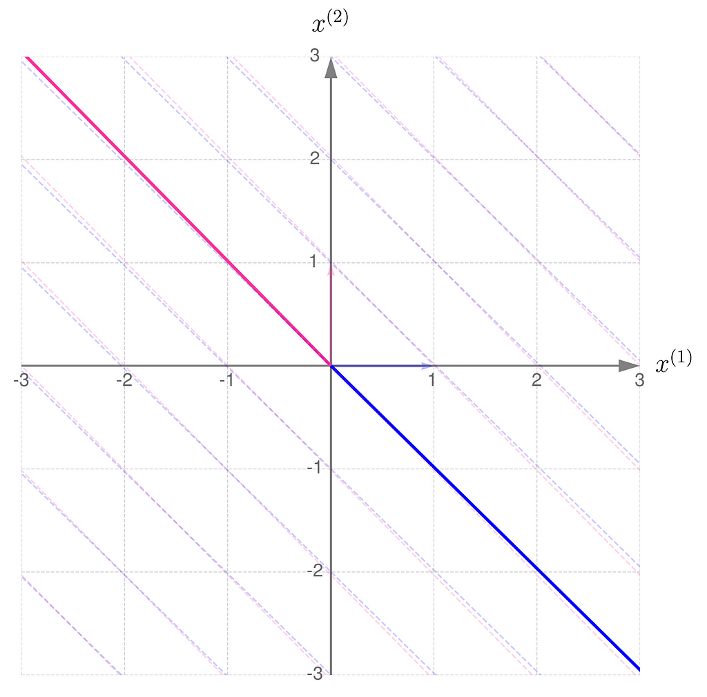
7. Non-invertible transformations
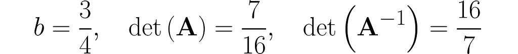
The workhorse of the next experiment will be the matrix with 1s on the diagonal and b on the antidiagonal:
where b is a fraction in the interval (0, 1). This matrix is, by definition, symmetrical, as it happens to be identical to its own transpose: A=Aᵀ, but I’m just mentioning this by the way; it’s not particularly relevant here.
Invert this matrix using the Gauss-Jordan method, and you will get the following:
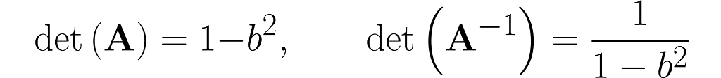
You can easily find online the rules for calculating the determinant of 2×2 matrices, which will give
This is no coincidence. In general, it holds that
Notice that when b = 0, the two matrices are identical. This is no surprise, as A reduces to the identity matrix I.
Things get tricky when b = 1, as the det(A) = 0 and det(A⁻¹) becomes infinite. As a result, A⁻¹ does not exist for a matrix A consisting entirely of 1s. In algebra classes, teachers often warn you about a zero determinant. However, when we consider where the matrix comes from, it becomes apparent that an infinite determinant can also occur, resulting in a fatal error. Anyway,
a zero determinant means the transformation is non-ivertible.
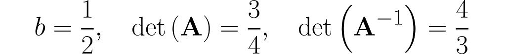
Now, the stage is set for experiments with different values of b. We’ve just seen how calculations fail at the limits, so let’s now visually investigate what happens as we carefully approach them.
We start with b = ½ and end up near 1.
Step 1)
Transformation ATransformation A⁻¹
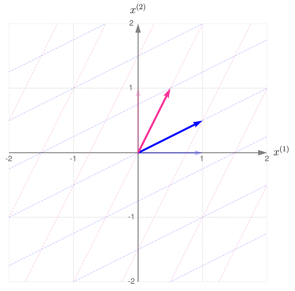
Step 2)
Transformation ATransformation A⁻¹
Recall that the determinant of the matrix representing the transformation corresponds to the area of the parallelogram formed by the transformed basis vectors.
This is in line with the illustrations: the smaller the area of the parallelogram for transformation A, the larger it becomes for transformation A⁻¹. What follows is: the narrower the basis for transformation A, the wider it is for its inverse. Note also that I had to extend the range on the axes because the basis vectors for transformation A are getting longer.
By the way, notice that
the transformation A has the same eigen-directions as A⁻¹.
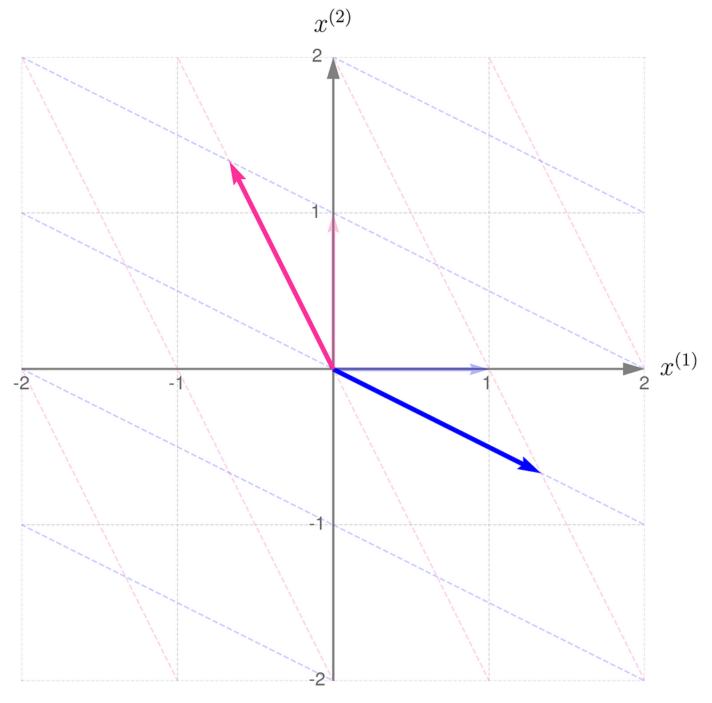
Step 3) Almost there…
Transformation ATransformation A⁻¹
The gridlines are squeezed so much that they almost overlap, which eventually happens when b hits 1. The basis vectors of are stretched so far that they go beyond the axis limits. When b reaches exactly 1, both basis vectors lie on the same line.
Having seen the previous illustrations, you’re now ready to guess the effect of applying a non-invertible transformation to the vectors. Take a moment to think it through first, then either try running a computational experiment or check out the results I’ve provided below.
.
.
.
Think of it this way.
When the basis vectors are not parallel, meaning they form an angle other than 0 or 180 degrees, you can use them to address any point on the entire plane (mathematicians say that the vectors span the plane). Otherwise, the entire plane can no longer be spanned, and only points along the line covered by the basis vectors can be addressed.
.
.
.
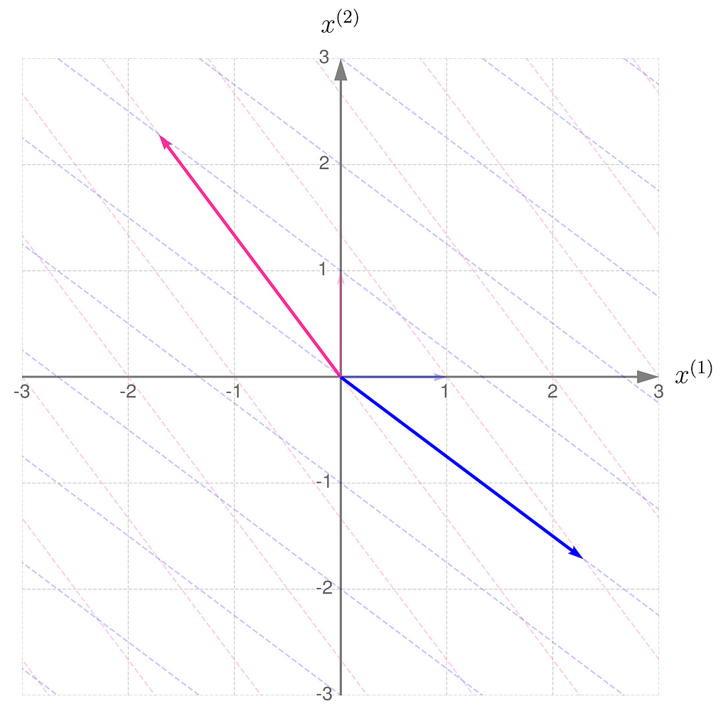
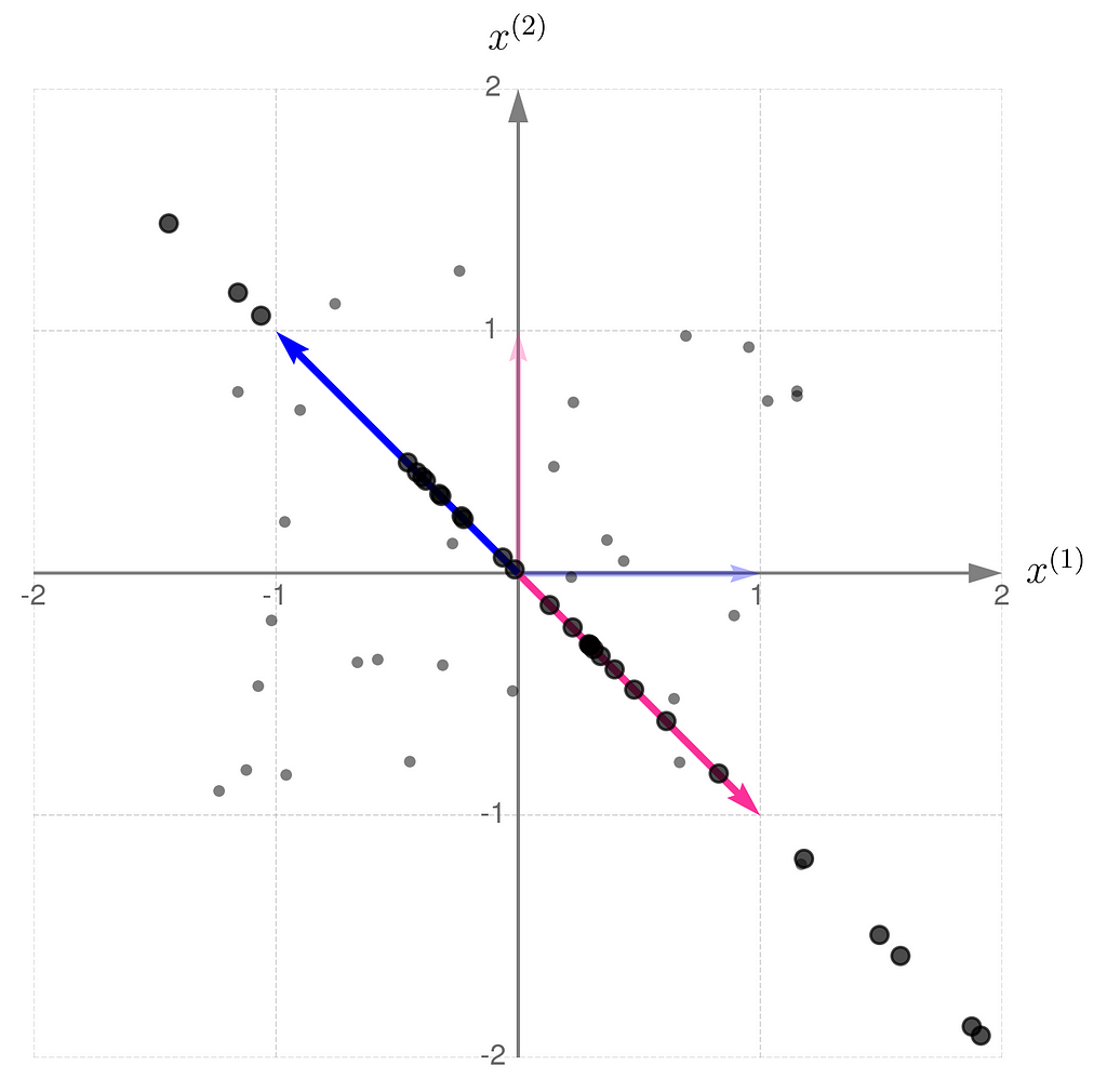
This is what it looks like when you apply the non-invertible transformation to randomly selected points:
A non-invertible matrix A reduces the dimensionality of the data
A consequence of applying a non-invertible transformation is that the two-dimensional space collapses to a one-dimensional subspace. After the transformation, it is no longer possible to uniquely recover the original coordinates of the points.
Take a look at the entries of matrix A. When b = 1, both columns (and rows) are identical, implying that the transformation matrix effectively behaves as if it were a 1 by 2 matrix, mapping two-dimensional vectors to a scalar.
You can easily verify that the problem would be the same if one row were a multiple of the other. This can be further generalized for matrices of any dimensions: if any row can be expressed as a weighted sum (linear combination) of the others, it implies that a dimension collapses. The reason is that such a vector lies within the space spanned by the other vectors, so it does not provide any additional ability to address points beyond those that can already be addressed. You may consider this vector redundant.
From section 4 on transposition, we can infer that if there are redundant rows, there must be an equal number of redundant columns.
8. Determinant
You might now ask if there’s a non-geometrical way to verify whether the columns or rows of the matrix are redundant.
Recall the parallelograms from Section 4 and the scalar quantity known as the determinant. I mentioned that
the determinant of a matrix indicates how the area of a unit parallelogram changes under the transformation.
The exact definition of the determinant is somewhat tricky, but as you’ve already seen, its graphical interpretation should not cause any problems.
I will demonstrate the behavior of two transformations represented by matrices:
det(A) = 2det(B) = -3/4
The magnitude of the determinant indicates how much the transformation stretches (if greater than 1) or shrinks (if less than 1) the space overall. While the transformation may stretch along one direction and compress along another, the overall effect is given by the value of the determinant.
Also, a negative determinant indicates a reflection; note that matrix B reverses the order of the basis vectors.
A parallelogram with zero area corresponds to a transformation that collapses a dimension, meaning the determinant can be used to test for redundancy in the basis vectors of a matrix.
Since the determinant measures the area of a parallelogram under a transformation, we can apply it to a sequence of transformations. If det(A) and det(B) represent the scaling factors of unit areas for transformations A and B, then the scaling factor for the unit area after applying both transformations sequentially, that is, AB, is equal to det(AB). As both transformations act independently and one after the other, the total effect is given by det(AB) = det(A) det(B). Substituting matrix A⁻¹ for matrix B and noting that det(I) = 1 leads to equation (5) introduced in the previous section.
Here’s how you can calculate the determinant using NumPy:
import numpy as np

A = np.array([
    [-1/2, 1/4],
    [2, 1/2]
    ])

print(f'det(A) = {np.linalg.det(A)}')
det(A) = -0.75
9. Non-square matrices
Until now, we’ve focused on square matrices, and you’ve developed a geometric intuition of the transformations they represent. Now is a great time to expand these skills to matrices with any number of rows and columns.
Wide matrices
This is an example of a wide matrix, which has more columns than rows:
From the perspective of equation (1), y = Ax, it maps three-dimensional vectors x to two-dimensional vectors y.
In such a case, one column can always be expressed as a multiple of another or as a weighted sum of the others. For example, the third column here equals 3/4 times the first column plus 5/4 times the second.
Once the vector x has been transformed into y, it’s no longer possible to reconstruct the original x from y. We say that the transformation reduces the dimensionality of the input data. These types of transformations are very important in machine learning.
Sometimes, a wide matrix disguises itself as a square matrix, but you can reveal it by checking whether its determinant is zero. We’ve had this situation before, remember?
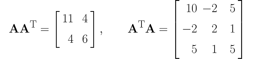
We can use the matrix A to create two different square matrices. Try deriving the following result yourself:
and also determinants (I recommend simplified formulas for working with 2×2 and 3×3 matrices):
The matrix AᵀA is composed of the dot products of all possible pairs of columns from matrix A, some of which are definitely redundant, thereby transferring this redundancy to AᵀA.
Matrix AAᵀ, on the other hand, contains only the dot products of the rows of matrix A, which are fewer in number than the columns. Therefore, the vectors that make up matrix AAᵀ are most likely (though not entirely guaranteed) linearly independent, meaning that one vector cannot be expressed as a multiple of another or as a weighted sum of the others.
What would happen if you insisted on determining x from y, which was previously computed as y = Ax? You could left-multiply both sides by A⁻¹ to get equation A⁻¹y = A⁻¹Ax and, since A⁻¹A = I, obtain x = A⁻¹y. But this would fail from the very beginning, because matrix A⁻¹, being non-square, is certainly non-invertible (at least not in the sense that was previously introduced).
However, you can extend the original equation y = Ax to include a square matrix where it’s needed. You just need to left-multiply matrix Aᵀ on both sides of the equation, yielding Aᵀy = AᵀAx. On the right, we now have a square matrix AᵀA. Unfortunately, we’ve already seen that its determinant is zero, so it appears that we have once again failed to reconstruct x from y.
Tall matrices
Here is an example of a tall matrix
that maps two-dimensional vectors x into three-dimensional vectors y. I made a third row by simply squaring the entries of the first row. While this type of extension doesn’t add any new information to the data, it can surprisingly improve the performance of certain machine learning models.
You might think that, unlike wide matrices, tall matrices allow the reconstruction of the original x from y, where y = Bx, since no information is discarded — only added.
And you’d be right! Look at what happens when we left-multiply by matrix Bᵀ, just like we tried before, but without success: Bᵀy = BᵀBx. This time, matrix BᵀB is invertible, so we can left-multiply by its inverse:
(BᵀB)⁻¹Bᵀy = (BᵀB)⁻¹(BᵀB)x
and finally obtain:
This is how it works in Python:
import numpy as np

# Tall matrix
B = [
    [2, -3],
    [1 , 0],
    [3, -3]
]

# Convert to numpy array
B = np.array(B)

# A column vector from a lower-dimensional space
x = np.array([-3,1]).reshape(2,-1)

# Calculate its corresponding vector in a higher-dimensional space
y = B @ x

reconstructed_x = np.linalg.inv(B.T @ B) @ B.T @ y

print(reconstructed_x)
[[-3.]
 [ 1.]]
To summarize: the determinant measures the redundancy (or linear independence) of the columns and rows of a matrix. However, it only makes sense when applied to square matrices. Non-square matrices represent transformations between spaces of different dimensions and necessarily have linearly dependent columns or rows. If the target dimension is higher than the input dimension, it’s possible to reconstruct lower-dimensional vectors from higher-dimensional ones.
10. Inverse and Transpose: similarities and differences
You’ve certainly noticed that the inverse and transpose operations play a key role in matrix algebra. In this section, we bring together the most useful identities related to these operations.
Whenever I apply the inverse operator, I assume that the matrix being operated on is square.
We’ll start with the obvious one that hasn’t appeared yet.
Here are the previously given identities (2) and (5), placed side by side:
Let’s walk through the following reasoning, starting with the identity from equation (4), where A is replaced by the composite AB:
The parentheses on the right are not needed. After removing them, I right-multiply both sides by the matrix B⁻¹ and then by A⁻¹.
Thus, we observe the next similarity between inversion and transposition (see equation (3)):
You might be disappointed now, as the following only applies to transposition.
But imagine if A and B were scalars. The same for the inverse would be a mathematical scandal!
For a change, the identity in equation (4) works only for the inverse:
I’ll finish off this section by discussing the interplay between inversion and transposition.
From the last equation, along with equation (3), we get the following:
Keep in mind that Iᵀ = I. Right-multiplying by the inverse of Aᵀ yields the following identity:
11. Translation by a vector
You might be wondering why I’m focusing only on the operation of multiplying a vector by a matrix, while neglecting the translation of a vector by adding another vector.
One reason is purely mathematical. Linear operations offer significant advantages, such as ease of transformation, simplicity of expressions, and algorithmic efficiency.
A key property of linear operations is that a linear combination of inputs leads to a linear combination of outputs:
where α, β are real scalars, and Lin represents a linear operation.
Let’s first examine the matrix-vector multiplication operator Lin[x] = Ax from equation (1):
This confirms that matrix-vector multiplication is a linear operation.
Now, let’s consider a more general transformation, which involves a shift by a vector b:
Plug in a weighted sum and see what comes out.
You can see that adding b disrupts the linearity. Operations like this are called affine to differentiate them from linear ones.
Don’t worry though — there’s a simple way to eliminate the need for translation. Simply shift the data beforehand, for example, by centering it, so that the vector b becomes zero. This is a common approach in data science.
Therefore, the data scientist only needs to worry about matrix-vector multiplication.
12. Final words
I hope that linear algebra seems easier to understand now, and that you’ve got a sense of how interesting it can be.
If I’ve sparked your interest in learning more, that’s great! But even if it’s just that you feel more confident with the course material, that’s still a win.
Bear in mind that this is more of a semi-formal introduction to the subject. For more rigorous definitions and proofs, you might need to look at specialised literature.
Unless otherwise noted, all images are by the author
References
[1] Gilbert Strang. Introduction to linear algebra. Wellesley-Cambridge Press, 2022.
[2] Marc Peter Deisenroth, A. Aldo Faisal, Cheng Soon Ong. Mathematics for machine learning. Cambridge University Press, 2020.
Surveying and improving the current methodologies for customer profiling
***To understand this article, knowledge of embeddings, clustering, and recommendation systems is required. The implementation of this algorithm has been released on GitHub and is fully open-source. I am open to criticism and welcome any feedback.
Most platforms, nowadays, understand that tailoring individual choices for each customer leads to increased user engagement. Because of this, the recommender systems’ domain has been constantly evolving, witnessing the birth of new algorithms every year.
hierarchical clustering, image by Author
Unfortunately, no existing taxonomy is keeping track of all algorithms in this domain. While most recommendation algorithms, such as matrix factorization, employ a neural network to make recommendations based on a list of choices, in this article, I will focus on the ones that employ a vector-based architecture to keep track of user preferences.
Exemplar Recommenders
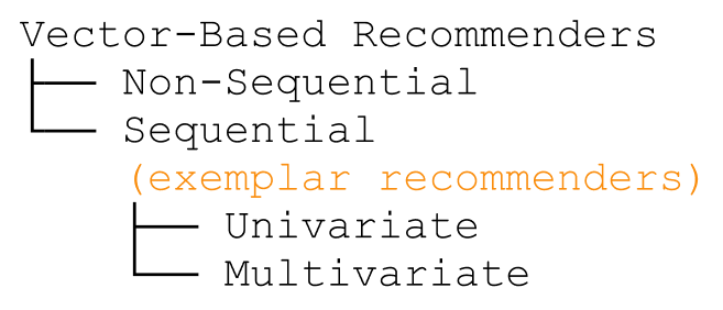
Thanks to the simplicity of embeddings, each sample that can be recommended (ex. products, content…) is converted into a vector using a pre-trained neural network (for example a matrix factorization): we can then use knn to make recommendations of similar products/customers. The algorithms following this paradigm are known as vector-based recommender systems. However, when these models take into consideration the previous user choices, they add a sequential layer to their base architecture and become technically known as vector-basedsequential recommenders. Because these architectures are becoming increasingly difficult (to both remember and pronounce), I am calling them exemplar recommenders: they extract a set of representative vectors from an initial set of choices to represent a user vector.
subdivision of recommender systems, image by Author
One of the first systems built on top of this architecture is Pinterest, which is running on top of its Pinnersage Recommendation engine: this scaled engine capable of managing over 2 Billion pins runs its own specific architecture and performs clustering on the choices of each individual user. As we can imagine, this represents a computational challenge when scaled. Especially after discovering covariate encoding, I would like to introduce four complementary architectures (two in particular, with the article’s name) that can relieve the stress of clustering algorithms when trying to profile each customer. You can refer to the following diagram to differentiate between them.
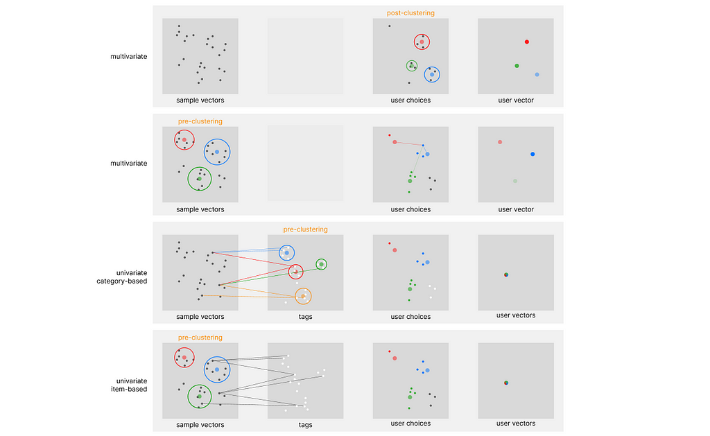
summary of exemplar recommenders, image by Author
Note that all the above approaches are classified as content-based filtering, and not collaborative filtering. In regards to the exemplar architecture, we can identify two main defining parameters: in-stack clustering implementation (we either perform clustering on the sample embedding or directly on the user embedding), and the number of vectors used to store user preferences over time.
In-Stack Clustering implementation
Using once again Pinnersage as an example, we can see how it performs a novel clustering iter for each user. However advantageous from an accuracy perspective, this is computationally very heavy.
Post-Clustering
When clustering is used on top of the user embeddings, we can refer to this approach (in this specific stack) as post-clustering. However inefficient this may look, applying a non-parametric clustering algorithm on billions of samples is borderline impossible, and probably not the best option.
Pre-Clustering
There might be some use cases when applying clustering on top of the sample data could be advantageous: we can refer to this approach (in this specific stack) as pre-clustering. For example, a retail store may need to track the history of millions of users, requiring the same computational resources of the Pinnersage architecture.
However, the number of samples of a retail store, compared to the Pinterest platform, should not exceed 10.000, against the staggering 2 Billion in comparison. With such a small number of samples, performing clustering on the sample embedding is very efficient, and will relieve the need to use it on the user embedding, if utilized properly.
Introducing the Univariate Architecture
As mentioned, the biggest challenge when creating these architectures is scalability. Each user amounts to hundreds of past choices held in record that need to be computed for exemplar extraction.
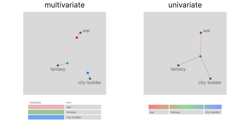
Multivariate architecture
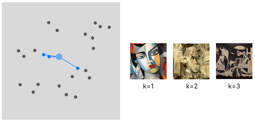
The most common way of building a vector-based recommender is to pin every user choice to an existing pre-computed vector. However, even if we resort to decay functions to minimize the number of vectors to take into account for our calculation, we still need to fill the cache with all the vectors at the time of our computation. In addition, at the time of retrieval, the vectors cannot be stored on the machine that performs the calculation, but need to be queried from a database: this sets an additional challenge for scalability.
The flow of this approach is the limited variance in recommendations. The recommended samples will be spatially very close to each other (the sample variance is minimized) and will only belong to the same category (unless there is in place a more complex logic defining this interaction).
multivariate exemplar recommendation, image by Author
WHEN TO USE: This approach (I am only taking into account the behavior of the model, not its computational needs) is suited for applications where we can recommend a batch of samples all from the same category. Art or social media applications are one example.
Univariate architecture
With this novel approach, we can store each user choice using a single vector that keeps updating over time. This should prove to be a remarkable improvement in scalability, minimizing the computational stress derived from both knn and retrieval.
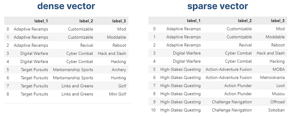
To make it even more complicated, there are two indexes where we can perform clustering. We can either cluster the items or the categories (both labeled using tags). There is no superior approach, we have to choose one depending on our use case.
> category-based
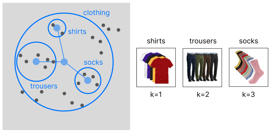
This article is entirely based on the construction of a category-based model. After tagging our data we can perform a clustering to group our data into a hierarchy of categories (in case our data is already organized into categories, there is no need to apply hierarchical clustering).
The main advantage of this approach is that the exemplar indicating the user preferences will be linked to similar categories (increasing product variance).
univariate category-based exemplar recommendation, image by Author
WHEN TO USE: Sometimes, we want to focus on recommending an entire category to our customers, rather than individual products. For example, if our user enjoys buying shirts (and by chance the exemplar is located in the latent region of red shirts), we would benefit more from recommending him the entire clothing category, rather than only red shirts. This approach is best suited for retail and fashion companies.
> item-based
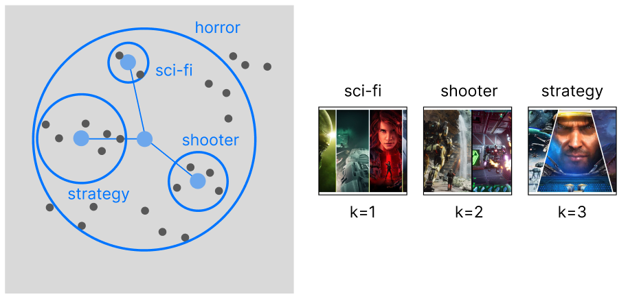
With an item-based approach, we are performing clustering on top of our samples. This will allow us to capture more granular information on the data, rather than focusing on separated categories: we want to expand beyond the limitations of the product categorization and recommend items across existing categories.
univariate item-based exemplar recommendation, image by Author
WHEN TO USE: The best companies that can make the best use for this approach are human resources and retailers with cross-categorical products (ex. videogames).
Univariate Exemplar Recommenders
Finally, we can explain in depth the architecture behind the category-based approach. This algorithm will perform exemplar extraction by only storing a single vector over time: the only technology capable of managing it is covariate encoding, hence we will use tags on top of the data. Because it uses pre-clustering, it is ideal for use cases with a manageable number of samples, but an unlimited number of users.
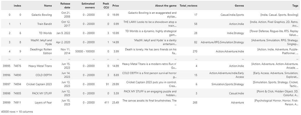
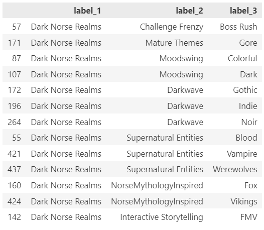
For this example, I will be using the open-source collection of the Steam game library (downloadable from Kaggle — MIT License), which is a perfect use case for this recommender at scale: Steam uses no more than 450 tags, and the number can occasionally increase over time; yet, it is manageable. This set of tags can be clustered very easily, and can even allow for manual intervention if we question the cluster assignment. Last, it serves millions of users, proving to be a realistic use case for our recommender.
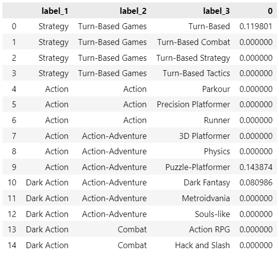
Sample of the Steam game dataset, image by Author
Its architecture can be articulated into the following phases: ***Note that when creating the sample code of this architecture I am using LLMs to make the entire process free from any human supervision. However, LLMs remain optional, and while they may improve the level of this recommender system, they are not an essential part of it.
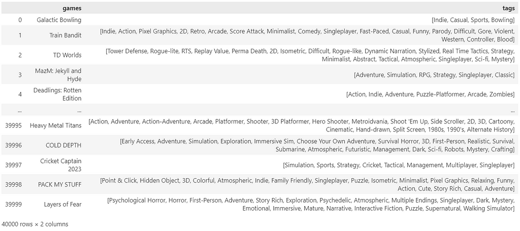
Sample Labeling We need to make sure to assign tags to each of our samples. Because of semantic tag filtering, we do not need to resort to zero-shots, but we can let a LLM manage this process without any supervision.
Pre-Clustering We are going to divide the tag embedding into different clusters. For a higher level of accuracy, we are going to use hierarchical clustering with a depth of 3.
Cluster labeling Once we have defined our cluster tree, we need to label each generated supercluster. We can still use LLM for this purpose. If you decide to avoid using LLMs, not that clusters can remain in a numerical form (this may only alter the user perception of the recommender).
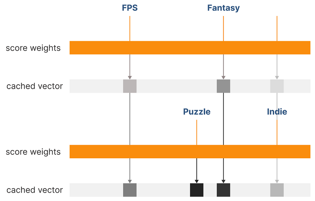
Balance non-uniform tag frequency The first challenge in picking from a list of tags is that the tags that appear the most (and are assigned to one cluster), heavily skew the recommender to propose that very cluster. We need to make sure that each cluster has the same probability of being recommended. We can achieve this by adding a custom multiplier that uniforms the probability of each cluster being recommended.
Univariate sequential encoding Now that our encoding weights have been defined, we can encode the user history in a vector, but with the possibility of updating it over time (using a decay function to get rid of old user preferences).
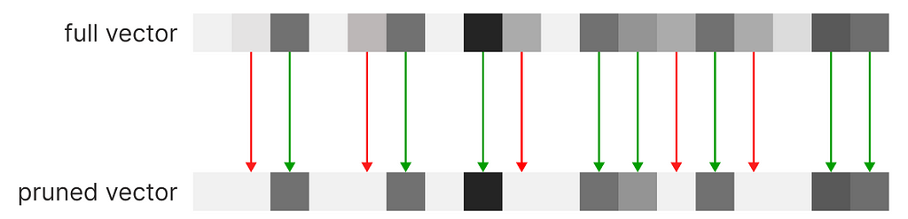
Account for scalability: pruning mechanism Because the dimensions of our vector are equivalent to the number of tags, we need to find a way to limit the size of the vector over time. PCA is a valid option, but because of the sum operations on the vector, feature pruning has proved to be more efficient.
Exemplar estimation This is where the innovation lies. We can encode the user profile as a single exemplar and still obtain separate cluster recommendations without any information loss that would arise IF we were to average multiple exemplars. This means that each of the previous multivariate methods would be incompatible with this architecture.
Let us begin with the full explanation behind the Univariate Exemplar Recommender:
1. Sample Labeling
In our reference dataset all samples have already been labeled using tags. If by any chance we are working with labeled data, we can easily do that using a LLM, prompting a request for a list of tags for each sample. As explained in my article on semantic tag filtering, we do not need to use zero-shots to guide the choice of labels, and the process can be completely unsupervised.
Screenshot of our sample data, each sample labeled with tags, image by Author
2. Pre-Clustering
As mentioned, the idea behind this recommender is to first organize the data into clusters, and then identify the most common clusters (exemplars) that define the preferences of every single user. Because the data is ideally very small (thousands of tags against billions of samples), clustering is no longer a burden and can be done on the tag embedding, rather than on the millions of user embeddings.
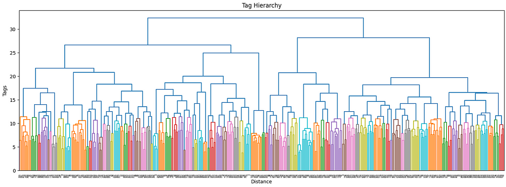
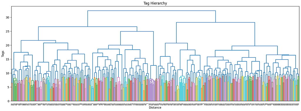
The more the number of tags increases, the more it makes sense to use a hierarchical structure to manage its complexity. Ideally, I would want not only to keep track of the main interests of each user but also their sub-interests and make recommendations accordingly. By using a dendrogram, we can define the different levels of clusters by using a threshold level.
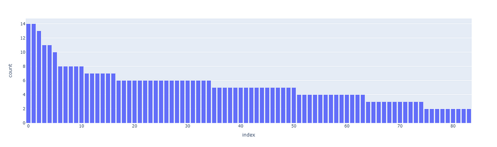
The first superclusters (level 1) will be the result of using a threshold of 11.4, resulting in the first 81 clusters. We can also see how their distribution is non-uniform (some clusters are bigger than others), but all considered, is not excessively skewed.
hierarchical clustering, level 1, threshold=11.4, image by Authorall the cluster sizes of level 1 clustering, image by Author
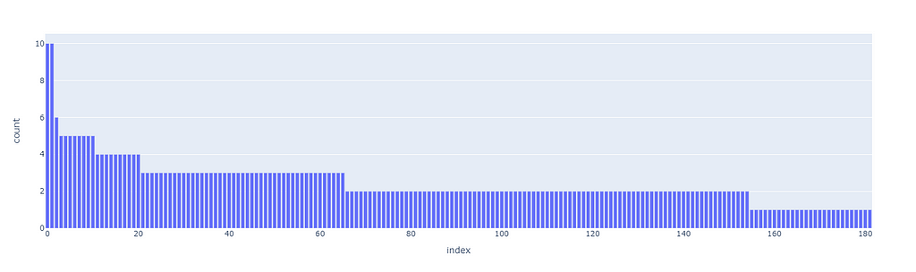
The next clustering level will be defined by a smaller threshold (9), which organizes the data in 181 clusters. Equivalently for the first level of clustering, the size distribution is uneven, but there are only two big clusters, so it should not be this big of an issue.
hierarchical clustering, level 2, threshold=9, image by Authorall the cluster sizes of level 2 clustering, image by Author
These thresholds have been arbitrarily chosen. Although there are non-parametric clustering algorithms that can perform the clustering process without any human input, they are quite challenging to manage, especially at scale, and show side effects such as the non-uniform distribution of cluster sizes. If among our clusters there are some that are too big (ex. one single cluster may even account for 20% of the overall data), then they may incorporate most recommendations without much sense.
Our priority when executing clustering is to obtain the most uniform distribution while maximizing the number of clusters so that the data can be split and differently represented as much as possible.
3. Cluster labeling
Because we have chosen to perform clustering on two levels of depths on top of our existing data, we have reached a total of 3 layers. The last layer is made by individual labels and is the only labeled layer. The other two, instead, only hold the cluster number without proper naming.
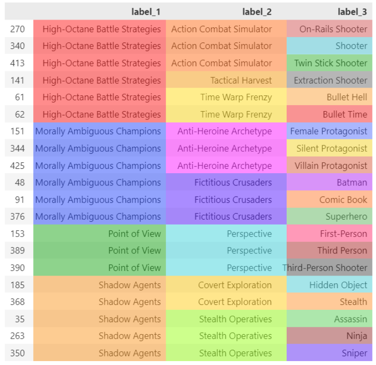
To solve this problem (note that this supercluster labeling step is not mandatory, but can improve how the user interacts with our recommender) we can use LLM on top of the superclusters. Let us try to automatically label all our clusters by feeding the tags inside of each group:
labeling for clusters at different depths, image by Author
Now that also our clusters have been labeled correctly, we can start building the foundation of our sequential recommender.
4. Balance non-uniform tag frequency
So far, we have completed the easy part. Now that we have all our elements ready to create a recommender, we still need to adjust the imbalances. It would be much more intuitive to showcase this step after the recommender is done, but, unfortunately, it is part of its base structure, you will need to bear this with me.
4.1 What if we skip balancing?
Let us, for a moment, skip ahead of time, and show the capabilities of our finished recommender by simply skipping this essential step. By assigning a score of 1 to each tag, there will be some tags that are so common that they will heavily skew the recommendation scores.
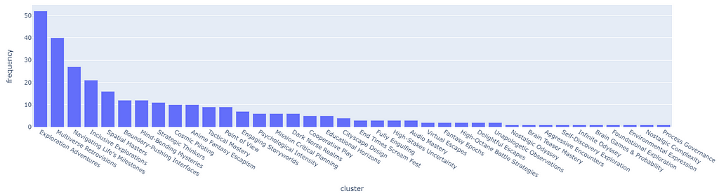
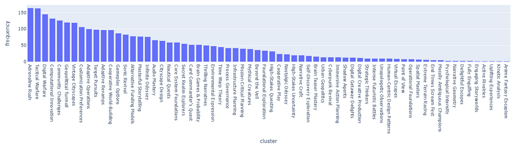
The following is a Monte Carlo simulation of 5000 random tag choices from the dataset. What we are looking at is the distribution of clusters that end up being chosen randomly after summing the scores. As we can see, the distribution is highly skewed and it will certainly break the recommender in favor of the clusters with the highest score.
recommended cluster frequency over 10k simulations, image by Author
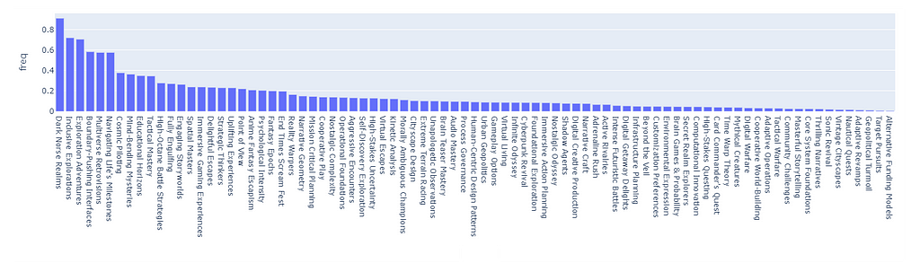
For example, the cluster “Dark Norse Realms” contains the tag Indie, which appears in 64% of all Samples (basically is almost impossible not to pick repetitively).
example of recommended clusters, image by Author
To be even more precise, let us directly simulate 100 different random sessions, each one picking the top 3 clusters from the session (the main user preference we keep track of), let us simulate entire user sessions so that the data is more complete. It is normal, especially when using a decay function, for the distribution to be non-uniform, and keep shifting over time.
recommended cluster frequency over 10k simulations, image by Author
However, if the skewness is excessive, the result is that the majority of users will be recommended the top 5% of the clusters 95% of the time (it is not precise numbers, just to prove my point).
4.2 Balancing probability distribution
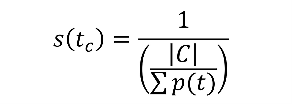
Instead, let us use a proper formula for frequency adjustment. Because the probability for each cluster is different, we want to assign a score that, when used to balance the weights of our user vector, will balance cluster retrieval:
scoring function to balance probability non-uniformity, image by Author
Let us look at the score assigned to each tag for 4 different random clusters:
example of recommended clusters, image by Author
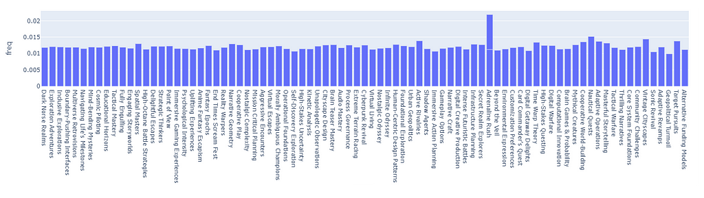
If we apply the score to the random pick (5000 picks, counting the frequency adjusted by the aforementioned weight), we can see how the tag distribution is now balanced (the outline ~ “Adrenaline Rush” is caused by a duplicate name):
cluster probability over 10k simulations, image by Author
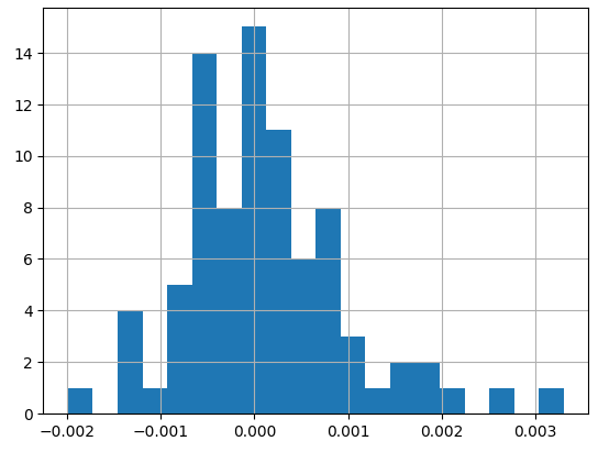
In fact, by looking at the normal distribution of the fluctuations, we see that the standard deviation for picking any cluster is approx. 0.1, which is extremely low (especially compared to before).
fluctuation distribution over 10k simulations, image by Author
By replicating 100 sessions, we see how, even with a pseudo-uniform probability distribution, the clusters amass over time following the Pareto principle.
recommended cluster frequency over 10k simulations, image by Author
5. Univariate sequential encoding
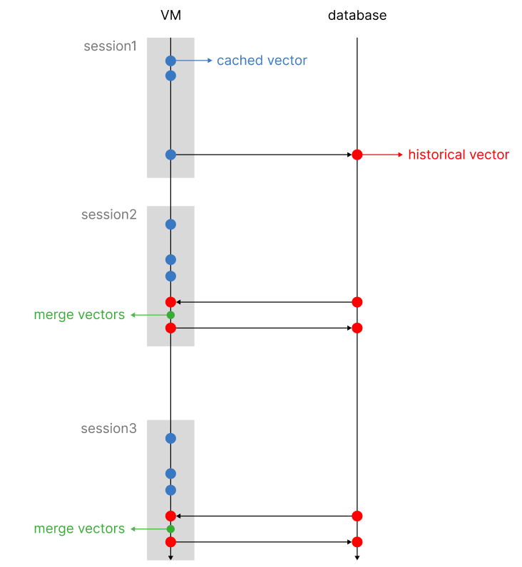
It is time to build the sequential mechanism to keep track of user choices over time. The mechanism I idealized works on two separate vectors (that after the process end up being one, hence univariate), a historical vector and a caching vector.
The historical vector is the one that is used to perform knn on the existing clusters. Once a session is concluded, we update the historical vector with the new user choices. At the same time, we adjust existing values with a decay function that diminishes the existing weights over time. By doing so, we make sure to keep up with the customer trends and give more weight to new choices, rather than older ones.
Rather than updating the vector at each user makes a choice (which is not computationally efficient, in addition, we risk letting older choices decay too quickly, as every user interaction will trigger the decay mechanism), we can store a temporary vector that is only valid for the current session. Each user interaction, converted into a vector using the tag frequency as one hot weight, will be summed to the existing cached vector.
vector sum workflow, image by Author
Once the session is closed, we will retrieve the historical vector from the database, merge it with the cached vector, and apply the adjustment mechanisms, such as the decay function and pruning, as we will see later). After the historical vector has been updated, it will be stored in the database replacing the old one.
session recommender workflow, image by Author
The two reasons to follow this approach are to minimize the weight difference between older and newer interactions and to make the entire process scalable and computationally efficient.
6. Pruning Mechanism
The system has been completed. However, there is an additional problem: covariate encoding has one flaw: its base vector is scaled proportionally to the number of encoded tags. For example, if our database were to reach 100k tags, the vector would have an equivalent number of dimensions.
The original covariate encoding architecture already takes this problem into account, proposing a PCA compression mechanism as a solution. However, applied to our recommender, PCA causes issues when iteratively summing vectors, resulting in information loss. Because every user choice will cause a summation of existing vectors with a new one, this solution is not advisable.
However, If we cannot compress the vector we can prune the dimensions with the lowest scores. The system will execute a knn based on the most relevant scores of the vector; this direct method of feature engineering won’t affect negatively (better yet, not excessively) the results of the final recommendation.
pruning mechanism, image by Author
By pruning our vector, we can arbitrarily set a maximum number of dimensions to our vectors. Without altering the tag indexes, we can start operating on sparse vectors, rather than a dense one, a data structure that only saves the active indexes of our vectors, being able to scale indefinitely. We can compare the recommendations obtained from a full vector (dense vector) against a sparse vector (pruned vector).
recommendation of the same user vector using a dense vs. sparse vector, image by Author
As we can see, we can spot minor differences, but the overall integrity of the vector has been maintained in exchange for scalability. A very intuitive alternative to this process is by performing clustering at the tag level, maintaining the vector size fixed. In this case, a tag will need to be assigned to the closest tag semantically, and will not occupy its dedicated dimension.
7. Exemplar estimation
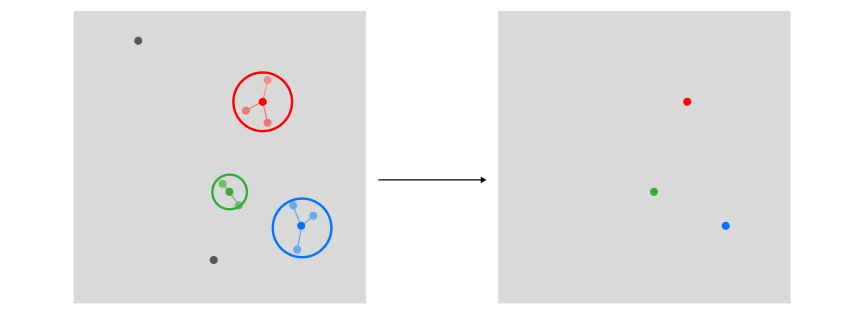
Now that you have fully grasped the theory behind this new approach, we can compare them more clearly. In a multivariate approach, the first step was to identify the top user preferences using clustering. As we can see, this process required us to store as many vectors as found exemplars.
Examplar extraction, image by Author
However, in a univariate approach, because covariate encoding works on a transposed version of the encoded data, we can use sections of our historical vector to store user preferences, hence only using a single vector for the entire process. Using the historical vector as a query to search through encoded tags: its top-k results from a knn search will be equivalent to the top-k preferential clusters.
difference between multivariate and univariate sets of vectors, image by Author
8. Recommendation approaches
Now that we have captured more than one preference, how do we plan to recommend items? This is the major difference between the two systems. The traditional multivariate recommender will use the exemplar to recommend k items to a user. However, our system has assigned our customer one supercluster and the top subclusters under it (depending on our level of tag segmentation, we can increase the number of levels). We will not recommend the top k items, but the top k subclusters.
Using groupby instead of vector search
So far, we have been using a vector to store data, but that does not mean we need to rely on vector search to perform recommendations, because it will be much slower than a SQL operation. Note that obtaining the same exact results using vector search on the user array is indeed possible.
If you are wondering why you would be switching from a vector-based system to a count-based system, it is a legitimate question. The simple answer to that is that this is the most loyal replica of the multivariate system (as portrayed in the reference images), but much more scalable (it can reach up to 3000 recommendations/s on 16 CPU cores using pandas). Originally, the univariate recommender was designed to employ vector search, but, as showcased, there are simpler and better search algorithms.
Simulation
Let us run a full test that we can monitor. We can use the code from the sample notebook: for our simple example, the user selects at least one game labeled with corresponding tags.
# if no vector exists, the first choices are the historical vector historical_vector = user_choices(5, tag_lists=[['Shooter', 'Fantasy']], tag_frequency=tag_frequency, display_tags=False)
At the end of 3 sessions, these are the top 3 exemplars (label_1) extracted from our recommender:
recommendation after 3 sessions, image by Author
In the notebook, you will find the option to perform Monte Carlo simulations, but there would be no easy way to validate them (mostly because team games are not tagged with the highest accuracy, and I noticed that most small games list too many unrelated or common tags).
Conclusion
The architectures of the most popular recommender systems still do not take into account session history, but with the development of new algorithms and the increase in computing power, it is now possible to tackle a higher level of complexity.
This new approach should offer a comprehensive alternative to the sequential recommender systems available on the market, but I am convinced that there is always room for improvement. To further enhance this architecture it would be possible to switch from a clustering-based to a network-based approach.
It is important to note that this recommender system can only excel when applied to a limited number of domains but has the potential to shine in conditions of scarce computational resources or extremely high demand.
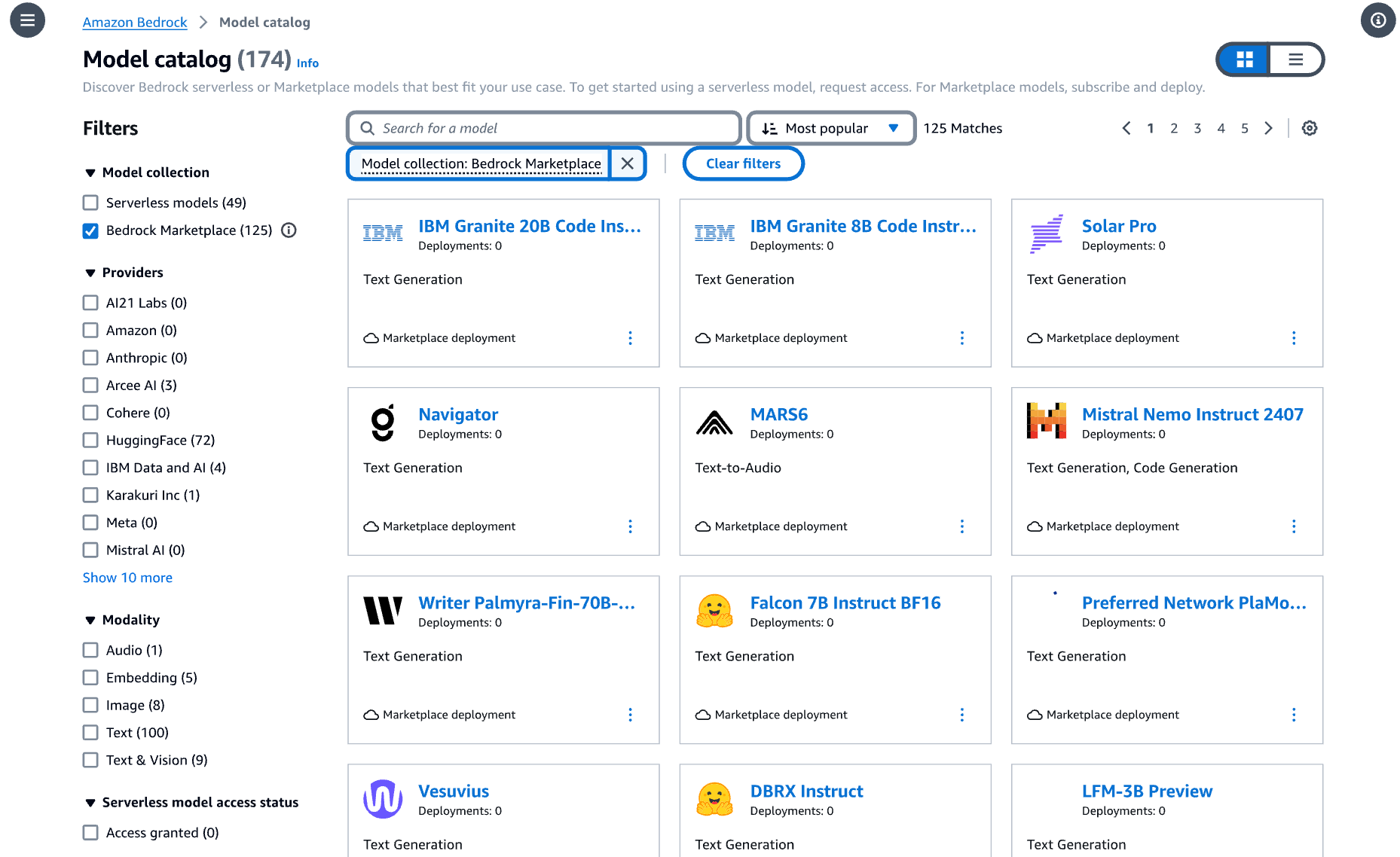
At AWS re:Invent 2024, we are excited to introduce Amazon Bedrock Marketplace. This a revolutionary new capability within Amazon Bedrock that serves as a centralized hub for discovering, testing, and implementing foundation models (FMs). In this post, we discuss the advantages and capabilities of Amazon Bedrock Marketplace and Nemotron models, and how to get started.
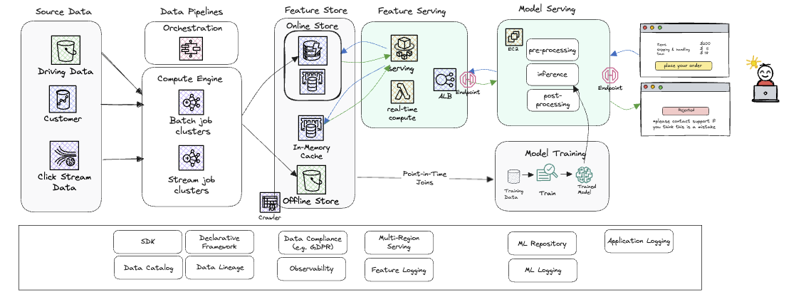
In this post, we discuss how Amazon SageMaker and Tecton work together to simplify the development and deployment of production-ready AI applications, particularly for real-time use cases like fraud detection. The integration enables faster time to value by abstracting away complex engineering tasks, allowing teams to focus on building features and use cases while providing a streamlined framework for both offline training and online serving of ML models.
In this post, we explore how to deploy AI models from SageMaker JumpStart and use them with Amazon Bedrock’s powerful features. Users can combine SageMaker JumpStart’s model hosting with Bedrock’s security and monitoring tools. We demonstrate this using the Gemma 2 9B Instruct model as an example, showing how to deploy it and use Bedrock’s advanced capabilities.
We use cookies on our website to give you the most relevant experience by remembering your preferences and repeat visits. By clicking “Accept”, you consent to the use of ALL the cookies.
This website uses cookies to improve your experience while you navigate through the website. Out of these, the cookies that are categorized as necessary are stored on your browser as they are essential for the working of basic functionalities of the website. We also use third-party cookies that help us analyze and understand how you use this website. These cookies will be stored in your browser only with your consent. You also have the option to opt-out of these cookies. But opting out of some of these cookies may affect your browsing experience.
Necessary cookies are absolutely essential for the website to function properly. These cookies ensure basic functionalities and security features of the website, anonymously.
Cookie
Duration
Description
cookielawinfo-checkbox-analytics
11 months
This cookie is set by GDPR Cookie Consent plugin. The cookie is used to store the user consent for the cookies in the category "Analytics".
cookielawinfo-checkbox-functional
11 months
The cookie is set by GDPR cookie consent to record the user consent for the cookies in the category "Functional".
cookielawinfo-checkbox-necessary
11 months
This cookie is set by GDPR Cookie Consent plugin. The cookies is used to store the user consent for the cookies in the category "Necessary".
cookielawinfo-checkbox-others
11 months
This cookie is set by GDPR Cookie Consent plugin. The cookie is used to store the user consent for the cookies in the category "Other.
cookielawinfo-checkbox-performance
11 months
This cookie is set by GDPR Cookie Consent plugin. The cookie is used to store the user consent for the cookies in the category "Performance".
viewed_cookie_policy
11 months
The cookie is set by the GDPR Cookie Consent plugin and is used to store whether or not user has consented to the use of cookies. It does not store any personal data.
Functional cookies help to perform certain functionalities like sharing the content of the website on social media platforms, collect feedbacks, and other third-party features.
Performance cookies are used to understand and analyze the key performance indexes of the website which helps in delivering a better user experience for the visitors.
Analytical cookies are used to understand how visitors interact with the website. These cookies help provide information on metrics the number of visitors, bounce rate, traffic source, etc.
Advertisement cookies are used to provide visitors with relevant ads and marketing campaigns. These cookies track visitors across websites and collect information to provide customized ads.