AI’s growing influence in large organizations brings crucial challenges in managing AI platforms. These include developing a scalable and operationally efficient platform that adheres to organizational compliance and security standards. Amazon SageMaker Studio offers a comprehensive set of capabilities for machine learning (ML) practitioners and data scientists. These include a fully managed AI development environment […]
The advent of transformers in 2017 set off a landslide of AI milestones, starting with the spectacular achievements of large language models (LLMs) in natural language processing (NLP), and quickly catalyzing advancement in other domains such as computer vision and robotics. The unification of NLP and computer vision problems into a common architecture accelerated efforts in learning joint vision-language representation spaces, which enabled the seminal achievements in vision-language modeling surrounding contrastive language-image pretraining (CLIP) in 2021, and lead to the birth of large multimodal models (LMMs).
This dawning era of large models has demonstrated awe-inspiring capabilities and marked several major strides toward artificial general intelligence (AGI), but the enormous size of these models makes them difficult to deploy. As with many transformative technologies before them, the alluring capabilities of LLMs were at first accessible only to those with the resources to operate at the bleeding edge of technology. While private research has continued to push the limits of performance using LMMs with hundreds of billions of parameters, open-source research has established a pattern of catching up to these watermarks using much smaller models.
Image by author. Over time, open-source LLMs are closing the performance gap with much smaller sizes.
Even with this increasing potency, however, the smallest LLMs will not fit on consumer GPUs for inference, let alone be trained, without model compression techniques being applied. Fortunately, the tantalizing capabilities of these models have driven researchers to find effective methods for squeezing them into smaller spaces. Thanks to their efforts, we can now deploy LLMs easily on consumer hardware, as well as fine-tune them to our desired use cases, without requiring the resources of the corporate titans. This series provides a comprehensive review of four model compression techniques that enable LLM inference and fine-tuning in resource-constrained environments, outlined below:
Model Compression Techniques for LLMs
Pruning — removal of network parameters individually (unstructured) or in groups (structured) based on their importance in order to decrease model complexity while maintaining accuracy.
Quantization — discretizing and/or reducing the resolution of the numeric space of the weights to save space and ease computation.
Knowledge Distillation — small models trained to target the learned functions of large experts can be trained with unlabeled data and outperform similar small models trained on the original task.
Parameter-Efficient Fine-Tuning — reduces the number of trainable parameters required to fine-tune a model for task-specific behavior.
Each of these techniques has been shown to greatly increase efficiency of large models with relatively innocuous effects on performance, bringing the awe-inspiring powers of the large pre-trained language model (PLM) colossus down to earth where they can be used by anyone. Here we explore each technique in detail, so that we are empowered to employ them in our own work. Like LLMs, these topics can only be compressed to a certain extent before significant loss of knowledge occurs. Hence, we will break this discussion into a series of articles to give each of these techniques the space it deserves, and properly review these rich legacies of research which together provide us with powerful channels for bringing fire to mankind.
In this article, we start at the beginning with the oldest technique on our list, almost as old as the backpropagation-trained neural networks that it compresses: pruning. First, a quick journey through the history of pruning will teach us the distinctions between unstructured and structured pruning techniques, along with their comparative strengths and weaknesses. Equipped with this prerequisite knowledge, we then review the application of these approaches in today’s world of LLMs, and offer closing thoughts.
The forthcoming installments in the Streamlining Giants series will provide similar dives into each of the remaining compression techniques: quantization, knowledge distillation, and parameter-efficient fine-tuning, elucidating a clear and comprehensive understanding of each so that we can approach the game of LLM development playing with a full deck.
Pruning
Image by author using DALL-E 3.
The quest to refine neural networks for practical applications traces its roots back to the foundational days of the field. When Rumelhart, Hinton, and Williams first demonstrated how to use the backpropagation algorithm to successfully train multi-layer neural networks that could learn complex, non-linear representations in 1986, the vast potential of these models became apparent. However, the computational power available in the 1980s restricted their practical use and the complexity of problems they could solve, a situation which mirrors the challenges we face with deploying LLMs today. Although the scale of models and the considerations being made were very different, early discoveries in network minimization would pave the way for big wins in model compression decades later. In this section, we take a brief journey through the history and motivations driving pruning research, discover the comparative strengths and weaknesses of unstructured versus structured methods, and prepare ourselves to explore their use in the modern era of LLMs.
Network pruning was originally motivated by the pursuit of better model generalization through freezing unimportant weights at zero, somewhat akin in theory to L1/Lasso and L2/Ridge regularization in linear regression, though different in that weights are selected and hard-set to zero (pruned) after training based on an importance criteria rather than being coaxed towards zero mathematically by the loss function during training (informed readers will know that regularization can also be achieved in neural network training using weight decay).
The common motivation behind both regularization and pruning (which can be seen as a form of regularization) is the theoretical and empirical evidence that neural networks are most effective at learning when overparameterized thanks to a higher-dimensional manifold of the loss function’s global minima and a larger exploration space in which effective subnetworks are more likely to be initialized (see “the lottery ticket hypothesis”). However, this overparameterization in turn leads to overfitting on the training data, and ultimately results in a network with many redundant or inactive weights. Although the theoretical mechanisms underlying the “unreasonable effectiveness” of overparameterized neural networks were less well studied at the time, researchers in the 1980s correctly hypothesized that it should be possible to remove a large portion of the network weights after training without significantly affecting task performance, and that performing iterative rounds of pruning and fine-tuning the remaining model weights should lead to better generalization, enhancing the model’s ability to perform well on unseen data.
Unstructured Pruning
To select parameters for removal, a measure of their impact on the cost function, or “saliency,” is required. While the earliest works in network minimization worked under the assumption that the magnitude of parameters should serve as a suitable measure of their saliency, LeCun et al. made a significant step forward in 1989 with “Optimal Brain Damage” (OBD), in which they proposed to use a theoretically justifiable measure of saliency using second-derivative information of the cost function with respect to the parameters, allowing them to directly identify the parameters which could be removed with the least increase in error.
Written in the era when the model of interest was a fully-connected neural network containing just 2,600 parameters, the authors of OBD were less concerned about removing weights due to computational efficiency than we are today with our billionaire behemoths, and were more interested in improving the model’s ability to generalize to unseen data by reducing model complexity. Even operating on a tiny model like this, however, the calculation of second-derivative information (Hessian matrix) is very expensive, and required the authors to make three convenient mathematical assumptions: 1) that the model is currently trained to an optimum, meaning the gradient of the loss with respect to every weight is currently zero and the slope of the gradient is positive in both directions, which zeroes out the first-order term of the Taylor expansion and implies the change in loss caused by pruning any parameter is positive, 2) that the Hessian matrix is diagonal, meaning the change in loss caused by removal of each parameter is independent, and therefore the loss deltas can be summed over subset of weights to calculate the total change in loss caused by their collective removal, and 3) that the loss function is nearly quadratic, meaning higher-order terms can be neglected from the Taylor expansion.
Results from OBD are superior to magnitude-based pruning (left). Accuracy of OBD saliency estimation (right).
Despite this requisite list of naïve assumptions, their theoretically justified closed-form saliency metric proved itself superior to magnitude-based pruning in accurately identifying the least important weights in a network, able to retain more accuracy at higher rates of compression. Nevertheless, the efficacy and profound simplicity of magnitude-based pruning methods would make them the top choice for many future research endeavors in model compression, particularly as network sizes began to scale quickly, and Hessians became exponentially more frightening. Still, this successful demonstration of using a theoretically justified saliency measure to more accurately estimate saliency and thereby enable more aggressive pruning provided an inspirational recipe for future victories in model compression, although it would be some time before those seeds bore fruit.
Results from OBD show that repeated iterations of pruning and fine-tuning preserve original performance levels even down to less than half the original parameter count. The implications in the context of today’s world of large models is clear, but they were more interested in boosting model generalization.
Four years later in 1993, Hassibi et al.’s Optimal Brain Surgeon (OBS) expanded on the concept of OBD and raised the levels of compression possible without increasing error by eschewing the diagonality assumption of OBD and instead considering the cross-terms within the Hessian matrix. This allowed them to determine optimal updates to the remaining weights based on the removal of a given parameter, simultaneously pruning and optimizing the model, thereby avoiding the need for a retraining phase. However, this meant even more complex mathematics, and OBS was thus initially of limited utility to 21st Century researchers working with much larger networks. Nonetheless, like OBD, OBS would eventually see its legacy revived in future milestones, as we will see later.
The pruning methods in OBD and OBS are examples of unstructured pruning, wherein weights are pruned on an individual basis based on a measure of their saliency. A modern exemplar of unstructured pruning techniques is Han et al. 2015, which reduced the sizes of the early workhorse convolutional neural networks (CNNs) AlexNet and VGG-16 by 9x and 13x, respectively, with no loss in accuracy, using one or more rounds of magnitude-based weight pruning and fine-tuning. Their method unfortunately requires performing sensitivity analysis of the network layers to determine the best pruning rate to use for each individual layer, and works best when retrained at least once, which means it would not scale well to extremely large networks. Nevertheless, it is impressive to see the levels of pruning which can be accomplished using their unstructured approach, especially since they are using magnitude-based pruning. As with any unstructured approach, the reduced memory footprint can only be realized by using sparse matrix storage techniques which avoid storing the zeroed parameters in dense matrices. Although they do not employ it in their study, the authors mention in their related work section that the hashing trick (as demonstrated in the 2015 HashedNets paper) is complementary to unstructured pruning, as increasing sparsity decreases the number of unique weights in the network, thereby reducing the probability of hash collisions, which leads to lower storage demands and more efficient weight retrieval by the hashing function.
Results from Han et al. 2015 show the power of unstructured pruning in CNNs of the time period. Notice the “free lunch” compression of 40–50% of parameters pruned away with no accuracy loss and no retraining.
While unstructured pruning has the intended regularization effect of improved generalization through reduced model complexity, and the memory footprint can then be shrunk substantially by using sparse matrix storage methods, the gains in computational efficiency offered by this type of pruning are not so readily accessed. Simply zeroing out individual weights without consideration of the network architecture will create matrices with irregular sparsity that will realize no efficiency gains when computed using dense matrix calculations on standard hardware. Only specialized hardware which is explicitly designed to exploit sparsity in matrix operations can unlock the computational efficiency gains offered by unstructured pruning. Fortunately, consumer hardware with these capabilities is becoming more mainstream, enabling their users to actualize performance gains from the sparse matrices created from unstructured pruning. However, even these specialized hardware units must impose a sparsity ratio expectation on the number of weights in each matrix row which should be pruned in order to allow for the algorithmic exploitation of the resulting sparsity, known as semi-structured pruning, and enforcing this constraint has been shown to degrade performance more than purely unstructured pruning.
Structured Pruning
We’ve seen that unstructured pruning is a well-established regularization technique that is known to improve model generalization, reduce memory requirements, and offer efficiency gains on specialized hardware. However, the more tangible benefits to computational efficiency are offered by structured pruning, which entails removing entire structural components (filters, layers) from the network rather than individual weights, which reduces the complexity of the network in ways that align with how computations are performed on hardware, allowing for gains in computational efficiency to be easily realized without specialized kit.
A formative work in popularizing the concept of structured pruning for model compression was the 2016 Li et al. paper “Pruning Filters for Efficient ConvNets,” where, as the title suggests, the authors pruned filters and their associated feature maps from CNNs in order to greatly improve computational efficiency, as the calculations surrounding these filters can be easily excluded by physically removing the chosen kernels from the model, directly reducing the size of the matrices and their multiplication operations without needing to worry about exploiting sparsity. The authors used a simple sum of filter weights (L1 norm) for magnitude-based pruning of the filters, demonstrating that their method could reduce inferences costs of VGG-16 and ResNet-110 by 34% and 38%, respectively, without significant degradation of accuracy.
Li et al. 2016 shows the effect of pruning convolutional filters from a CNN.
Their study also reveals some fascinating insights about how convolutional networks work by comparing the sensitivity of individual CNN layers to pruning, revealing that layers on the very beginning or past halfway through the depth of the network were able to be pruned aggressively with almost no impact on the model performance, but that layers around 1/4 of the way into the network were very sensitive to pruning and doing so made recovering model performance difficult, even with retraining. The results, shown below, reveal that the layers which are most sensitive to pruning are those containing many filters with large absolute sums, supporting the theory of magnitude as a saliency measure, as these layers are clearly more important to the network, since pruning them away causes pronounced negative impact on model performance which is difficult to recover.
Results from Li et al. 2016 reveal marked differences in the sensitivity of CNN layers to filter pruning.
Most importantly, the results from Li et al. show that many layers in a CNN could be pruned of even up to 90% of their filters without harming (and in some cases even improving) model performance. Additionally, they found that when pruning filters from the insensitive layers, iterative retraining layer-by-layer was unnecessary, and a single round of pruning and retraining (for 1/4 of the original training time) was all that was required to recover model performance after pruning away significant portions of the network. This is great news in terms of efficiency, since multiple rounds of retraining can be costly, and previous work had reported requiring up to 3x original training time to produce their pruned models. Below we can see the overall results from Li et al. which reveal that the number of floating point operations (FLOPs) could be reduced between 15 and 40 percent in the CNNs studied without harming performance, and in fact offering gains in many instances, setting a firm example of the importance of pruning models after training.
Results from Li et al. 2016 comparing their select pruning configurations to the baseline CNNs, evaluated on CIFAR-10 (top three models) and ImageNet (ResNet-34 section).
Although this study was clearly motivated by efficiency concerns, we know from decades of evidence linking reduced model complexity to improved generalization that these networks should perform better on unseen data as well, a fundamental advantage which motivated pruning research in the first place. However, this pruning method requires a sensitivity analysis of the network layers in order to be done correctly, requiring additional effort and computation. Further, as LeCun and his colleagues correctly pointed out back in 1989: although magnitude-based pruning is a time-tested strategy, we should expect a theoretically justified metric of salience to produce a superior pruning strategy, but with the size of modern neural networks, computing the Hessian matrix required for the second-order Taylor expansions used in their OBD method would be too intensive. Fortunately, a happy medium was forthcoming.
Trailing Li et al. by only a few months in late 2016, Molchanov and his colleagues at Nvidia reinvestigated the use of Taylor expansion to quantify salience for structured pruning of filters from CNNs. In contrast to OBD, they avoid the complex calculation of the second-order terms, and instead extract a useful measure of saliency by considering the variance rather than the mean of the first-order Taylor expansion term. The study provides empirical comparison of several saliency measures against an “oracle” ranking which was computed by exhaustively calculating the change in loss caused by removing each filter from a fine-tuned VGG-16. In the results shown below, we can see that the proposed Taylor expansion saliency measure most closely correlates with the oracle rankings, followed in second place by the more computationally intensive OBD, and the performance results reflect that these methods are also best at preserving accuracy, with the advantage more clearly in favor of the proposed Taylor expansion method when plotting over GFLOPs. Interestingly, the inclusion of random filter pruning in their study shows us that it performs surprisingly well compared to minimum weight (magnitude-based) pruning, challenging the notion that weight magnitude is a reliable measure of saliency, at least for the CNN architectures studied.
Results from Molchanov et al. 2016 show first-order Taylor expansion providing effective measure of filter saliency, representing the highest correlations with oracle ranking and best preservation of accuracy.
Pruning LLMs
Image by author using DALL-E 3.
After the widespread adoption of LLMs, researchers naturally moved to investigate the use of pruning on these architectures. Both unstructured and structured pruning can be successfully applied to LLMs to reduce their model size substantially with negligible drops in performance. As one might expect, however, the enormous size of these models requires special considerations to be made, since calculating saliency measures over models containing tens or hundreds of billions of weights is very costly, and retraining to recover model performance after pruning is prohibitively expensive. Thus, there is newfound motivation to perform pruning with as little retraining as possible, and to enforce simplicity in the saliency measures used for pruning.
Consistent with the previous eras of pruning research, it is apparent that LLMs can be pruned far more aggressively using unstructured as opposed to structured methods, but again the efficiency gains are more directly accessible with the latter. For practitioners with better access to specialized resources, exploiting the sparse matrices and massive compression rates provided by unstructured pruning may be the right choice, but for many people, the accessible efficiency gains on general hardware offered by structured pruning will be more appealing, despite the more modest levels of compression. In this section, we will review both approaches in today’s LLM landscape, so that we are equipped to make the best choice given our individual circumstances.
Unstructured Pruning of LLMs
In early 2023, SparseGPT was the first work to investigate unstructured pruning of GPT models with billions of parameters, proposing an efficient method using a novel approximate sparse regression solver to determine the prunable weights in models of this scale within a matter of hours, and demonstrating that the largest open source models of the day (≤175B) could be pruned to between 50% and 60% sparsity with minimal loss of accuracy in one shot without any retraining at all, significantly exceeding the results offered by magnitude-based approaches in the one-shot setting. Their approach takes an iterative perspective on OBS, finding that the same mathematical result can be broken down into a series of operations which are more efficient to compute. However, since their method is still an example of unstructured pruning, specialized hardware is necessary for realizing efficiency gains from their technique, and enforcing the required 2:4 or 4:8 semi-structured sparsity pattern expectation causes drops in performance compared to purely unstructured pruning.
Results from SparseGPT show clear advantage over magnitude based pruning (left), and demonstrate the detrimental effects of enforcing sparsity patterns to enable hardware optimization (right).
Later in mid-2023, the authors of Wanda postulated about why quantization had seen so much more research interest than pruning in the LLM era, whereas previously the two compression techniques were equally popular. They attributed this to the fact that up until SparseGPT, all pruning methods required retraining the LLM at some point, making them cost-prohibitive to anyone without the resources to do so, creating a significant deterrent to both research and practical adoption. While SparseGPT showed that one-shot pruning was possible, their iterative OBS approach is still quite computationally intensive. In this light, Wanda opts for a simple magnitude-based unstructured pruning method, which they augment by multiplying the weight magnitudes by the norm of their associated input activations creating a more descriptive and wholistic magnitude-based measure of saliency. The comparison chart below shows the saliency formulations and complexities of these unstructured approaches.
Table from Sun et al. 2023 compares unstructured pruning approaches for LLMs and their complexity.
Wanda’s approach also produces pruned models that are ready to use without any retraining, but as an unstructured approach, again requires special hardware for efficiency gains. Nevertheless, for those equipped to take advantage of unstructured pruning, Wanda’s approach matches or exceeds the results of SparseGPT while reducing complexity by an entire factor of the model’s hidden dimension, establishing it as a strong choice for the compression of LLMs.
Table from Sun et al. 2023 shows competitive performance with SparseGPT with a fraction of the complexity.
Structured Pruning of LLMs
Contemporaneously with Wanda, researchers at the National University of Singapore offered a structured pruning method called LLM-Pruner. In their study, they found it necessary to settle for a 20% pruning rate, since more aggressive pruning led to substantially degraded performance. Also, while it was necessary to retrain the weights after pruning to recover model performance, they were able to achieve this using low-rank adaptation (LoRA) in just 3 hours on 50k training samples. Although the efficiency of fine-tuning with LoRA is a relief, their method nonetheless requires gradients for the full model to be generated to measure parameter saliency before pruning, so while resource-constrained users may enjoy the pruned model, performing the operation themselves may not be possible.
Just slightly later in 2023, LoRAPrune improved on the effectiveness for structured pruning of LLMs substantially by using the gradients and weights of LoRA training to establish parameter importance in the larger network, and performing iterative rounds of pruning on both the network and corresponding LoRA weights. This method is able to prune the LLaMA-65B model on a single 80GB A100 GPU, thanks to depending on the gradients of the efficient low-rank parameter space rather than the full model. Since the LLM weights remain frozen during the process, they can be quantized to 8-bit to save memory with minimal impact on the results.
Helpful graphic from Zhang et al. 2023 depicts the structured pruning method used in LoRAPrune.
Although they came up against the same sensitivity of the LLM to more aggressive levels of structured pruning, the authors of LoRAPrune demonstrate through extensive experimentation that their method produced pruned models with superior performance compared to previous structured methods using only a fraction of the resources to perform the pruning operation.
Results from LoRAPrune demonstrate a clear advantage after fine-tuning compared with previous methods.
In October of 2023, researchers at Microsoft proposed LoRAShear, a structured pruning method which uses Dependency Graph Analysis on the LLM and progressive structured pruning via LoRA Half-Space Projected Gradient (LHSPG), which “transfers the knowledge stored in the relatively redundant structures to the important structures to better preserve the knowledge of the pretrained LLM.” Additionally, they go beyond the trend in previous works of performing only instruction-based fine-tuning to recover knowledge, and instead first adaptively create a subset from the pretraining datasets based on the resulting performance distribution to recover the general pretraining knowledge that was lost during pruning, and then proceeding to “perform the usual instructed finetuning to recover domain-specific expertise and the instruction capacity of pruned LLMs.” With their more involved approach, they achieve a mere 1% drop in performance at the 20% pruning rate, and maintain an unprecedented 82% of original performance at the 50% pruning rate.
Results from LoRAShear shows superior performance, albeit with a much more complex pruning algorithm.
Then in early 2024, the aptly named Bonsai demonstrated a superior method for structured pruning of LLMs using only forward pass information, drastically reducing the computational requirements for performing the pruning process by not requiring gradients, thereby empowering those most in need of pruned models to generate them within their resource-constrained environments. With their efficient approach, they are able to closely match the performance of LoRAShear in the instruction-tuned only condition, although it would appear the additional considerations made by LoRAShear do pay dividends in knowledge recovery, but the differing spreads of evaluation datasets used in the two studies unfortunately disallow for clear comparison. Interestingly, LoRAShear is unmentioned in the Bonsai paper, presumably for the reason that the additional levels of complexity in the former make for a muddy comparison with the more straightforward methods examined by the latter, but we are left to speculate. Nevertheless, Bonsai contributes a powerful and valuable step towards democratizing LLMs and their pruning by focusing on simplicity and efficiency, able to perform the pruning operation using only the amount of GPU memory needed to run inference for a given model, and achieves impressive results with the most accessible method of structured LLM pruning published so far.
Results from Dery et al. show Bonsai achieves superior performance to previous structured pruning methods.
Conclusion
Image by author using DALL-E 3.
In this article, we’ve journeyed through the history of network pruning, starting with the dawn of unstructured techniques in the late 1980s to the current trends in LLM applications. We’ve seen that pruning is broadly categorized as either unstructured or structured pruning, depending on whether the weights are considered individually or in groups, and that the latter, while only usable at lower compression rates, provides direct relief in computational burden. We saw that gains in efficiency can be realized in the unstructured setting, but only when special storage techniques and hardware are used, and that an additional “semi-structured” condition must be obeyed for the hardware acceleration to work, which comes at a cost in performance compared with pure unstructured pruning. Pure unstructured pruning provides the most stunning compression rates with no loss in accuracy, but the irregular sparsity created does not provide efficiency gains outside of storage size, making it less appealing in the context of democratizing LLMs.
We’ve explored the concept of saliency, which refers to the various measures of importance (saliency) by which model parameters can be pruned. The most simple and accessible estimation of saliency is weight magnitude, where weights closer to zero are assumed to be less important. Although this approach is not theoretically sound (as near-zero weights can indeed be important to model performance), it is still extremely effective, and the lack of complex calculations gives it persisting popularity. On the other hand, theoretically sound measures of saliency date back to the earliest days of trainable neural networks, and are proven to produce superior models compared to magnitude-based pruning, but the complex calculations required by these early methods don’t scale well to the size of today’s LLMs. Fortunately, motivated researchers in the modern era have found ways to calculate these saliency metrics more efficiently, but alas, they still require the calculation of the gradients. In the most recent work from 2024, Bonsai demonstrated that accurate pruning can be achieved without gradients, using only the information from the forward pass.
While modern pruning research is driven primarily by the interest of compressing the unwieldy sizes of today’s top performing models so that they can be deployed on reasonably sized hardware, pruning was originally motivated by the improved generalizability that results from reducing model complexity. This regularization effect is surely taking effect in pruned LLMs, which is presumably a benefit, but the actual impact of this is less studied in today’s literature. While improving model generalizability and reducing overfitting through regularization are known to be beneficial, there may be special considerations which need to be made in the context of LLMs, which are often expected to recall minute details in vast sums of training data, depending on the use case. Therefore, it would be fruitful for future work to investigate at what point this regularization starts to have deleterious effects on intended use cases of LLMs.
In the next episode…
The methods investigated in this article offer effective model compression through the removal of model parameters, known as pruning, but this is only one approach to model compression. In the next article, we will explore the concept of quantization at various resolutions, developing a functional knowledge of the subject within a reasonable memory footprint.
Streamlining Giants was originally published in Towards Data Science on Medium, where people are continuing the conversation by highlighting and responding to this story.
MusicLM, Google’s flagship text-to-music AI, was originally published in early 2023. Even in its basic version, it represented a major breakthrough and caught the music industry by surprise. However, a few weeks ago, MusicLM received a significant update. Here’s a side-by-side comparison for two selected prompts:
Prompt: “Dance music with a melodic synth line and arpeggiation”:
This increase in quality can be attributed to a new paper by Google Research titled: “MusicRL: Aligning Music Generation to Human Preferences”. Apparently, this upgrade was considered so significant that they decided to rename the model. However, under the hood, MusicRL is identical to MusicLM in its key architecture. The only difference: Finetuning.
What is Finetuning?
When building an AI model from scratch, it starts with zero knowledge and essentially does random guessing. The model then extracts useful patterns through training on data and starts displaying increasingly intelligent behavior as training progresses. One downside to this approach is that training from scratch requires a lot of data. Finetuning is the idea that an existing model is used and adapted to a new task, or adapted to approach the same task differently. Because the model already has learned the most important patterns, much less data is required.
For example, a powerful open-source LLM like Mistral7B can be trained from scratch by anyone, in principle. However, the amount of data required to produce even remotely useful outputs is gigantic. Instead, companies use the existing Mistral7B model and feed it a small amount of proprietary data to make it solve new tasks, whether that is writing SQL queries or classifying emails.
The key takeaway is that finetuning does not change the fundamental structure of the model. It only adapts its internal logic slightly to perform better on a specific task. Now, let’s use this knowledge to understand how Google finetuned MusicLM on user data.
How Google Gathered User Data
A few months after the MusicLM paper, a public demo was released as part of Google’s AI Test Kitchen. There, users could experiment with the text-to-music model for free. However, you might know the saying: If the product is free, YOU are the product. Unsurprisingly, Google is no exception to this rule. When using MusicLM’s public demo, you were occasionally confronted with two generated outputs and asked to state which one you prefer. Through this method, Google was able to gather 300,000 user preferences within a couple of months.
Example of the user preference ratings captured in the MusicLM public playground. Image taken from the MusicRL paper.
As you can see from the screenshot, users were not explicitly informed that their preferences would be used for machine learning. While that may feel unfair, it is important to note that many of our actions in the internet are being used for ML training, whether it is our Google search history, our Instagram likes, or our private Spotify playlists. In comparison to these rather personal and sensitive cases, music preferences on the MusicLM playground seem negligible.
Example of User Data Collection on Linkedin Collaborative Articles
It is good to be aware that user data collection for machine learning is happening all the time and usually without explicit consent. If you are on Linkedin, you might have been invited to contribute to so-called “collaborative articles”. Essentially, users are invited to provide tips on questions in their domain of expertise. Here is an example of a collaborative article on how to write a successful folk song (something I didn’t know I needed).
Header of a collaborative article on songwriting. On the right side, I am asked to contribute to earn a “Top Voice” badge.
Users are incentivized to contribute, earning them a “Top Voice” badge on the platform. However, my impression is that noone actually reads these articles. This leads me to believe that these thousands of question-answer pairs are being used by Microsoft (owner of Linkedin) to train an expert AI system on these data. If my suspicion is accurate, I would find this example much more problematic than Google asking users for their favorite track.
But back to MusicLM!
How Google Took Advantage of this User Data
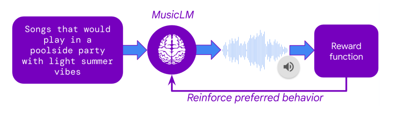
The next question is how Google was able to use this massive collection of user preferences to finetune MusicLM. The secret lies in a technique called Reinforcement Learning from Human Feedback (RLHF) which was one of the key breakthroughs of ChatGPT back in 2022. In RLHF, human preferences are used to train an AI model that learns to imitate human preference decisions, resulting in an artificial human rater. Once this so-called reward model is trained, it can take in any two tracks and predict which one would most likely be preferred by human raters.
With the reward model set up, MusicLM could be finetuned to maximize the predicted user preference of its outputs. This means that the text-to-music model generated thousands of tracks, each track receiving a rating from the reward model. Through the iterative adaptation of the model weights, MusicLM learned to generate music that the artificial human rater “likes”.
In addition to the finetuning on user preferences, MusicLM was also finetuned concerning two other criteria: 1. Prompt Adherence MuLan, Google’s proprietary text-to-audio embedding model was used to calculate the similarity between the user prompt and the generated audio. During finetuning, this adherence score was maximized. 2. Audio Quality Google trained another reward model on user data to evaluate the subjective audio quality of its generated outputs. These user data seem to have been collected in separate surveys, not in MusicLM’s public demo.
How Much Better is the New MusicLM?
The new, finetuned model seems to reliably outperform the old MusicLM, listen to the samples provided on the demo page. Of course, a selected public demo can be deceiving, as the authors are incentivized to showcase examples that make their new model look as good as possible. Hopefully, we will get to test out MusicRL in a public playground, soon.
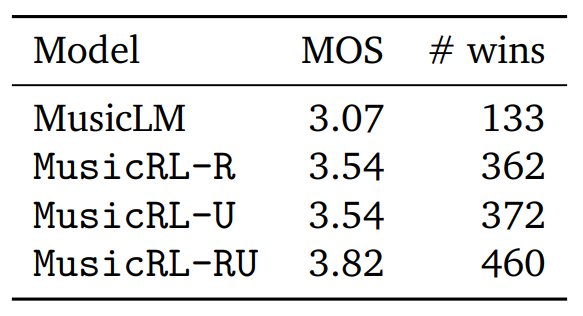
However, the paper also provides a quantitative assessment of subjective quality. For this, Google conducted a study and asked users to compare two tracks generated for the same prompt, giving each track a score from 1 to 5. Using this metric with the fancy-sounding name Mean Opinion Score (MOS), we can compare not only the number of direct comparison wins for each model, but also calculate the average rater score (MOS).
Quantitative benchmarks. Image taken from MusicRL paper.
Here, MusicLM represents the original MusicLM model. MusicRL-R was only finetuned for audio quality and prompt adherence. MusicRL-U was finetuned solely on human feedback (the reward model). Finally, MusicRL-RU was finetuned on all three objectives. Unsurprisingly, MusicRL-RU beats all other models in direct comparison as well as on the average ratings.
The paper also reports that MusicRL-RU, the fully finetuned model, beat MusicLM in 87% of direct comparisons. The importance of RLHF can be shown by analyzing the direct comparisons between MusicRL-R and MusicRL-RU. Here, the latter had a 66% win rate, reliably outperforming its competitor.
What are the Implications of This?
Although the difference in output quality is noticeable, qualitatively as well as quantitatively, the new MusicLM is still quite far from human-level outputs in most cases. Even on the public demo page, many generated outputs sound odd, rhythmically, fail to capture key elements of the prompt or suffer from unnatural-sounding instruments.
In my opinion, this paper is still significant, as it is the first attempt at using RLHF for music generation. RLHF has been used extensively in text generation for more than one year. But why has this taken so long? I suspect that collecting user feedback and finetuning the model is quite costly. Google likely released the public MusicLM demo with the primary intention of collecting user feedback. This was a smart move and gave them an edge over Meta, which has equally capable models, but no open platform to collect user data on.
All in all, Google has pushed itself ahead of the competition by leveraging proven finetuning methods borrowed from ChatGPT. While even with RLHF, the new MusicLM has still not reached human-level quality, Google can now maintain and update its reward model, improving future generations of text-to-music models with the same finetuning procedure.
It will be interesting to see if and when other competitors like Meta or Stability AI will be catching up. For us as users, all of this is just great news! We get free public demos and more capable models.
For musicians, the pace of the current developments may feel a little threatening — and for good reason. I expect to see human-level text-to-music generation in the next 1–3 years. By that, I mean text-to-music AI that is at least as capable at producing music as ChatGPT was at writing texts when it was released. Musicians must learn about AI and how it can already support them in their everyday work. As the music industry is being disrupted once again, curiosity and flexibility will be the primary key to success.
Interested in Music AI?
If you liked this article, you might want to check out some of my other work:
Histograms are widely used and easily grasped, but when it comes to estimating continuous densities, people often resort to treating it as a mysterious black box. However, understanding this concept is just as straightforward and becomes crucial, especially when dealing with bounded data like age, height, or price, where available libraries may not handle it automatically.
1. Kernel Density Estimation
Histogram
A histogram involves partitioning the data range into bins or sub-intervals and counting the number of samples that fall within each bin. It thus approximates the continuous density function with a piecewise constant function.
Large bin size: It helps capturing the low-frequency outline of the density function, by gathering neighboring samples to avoid empty bins. However, it looses the continuity property because there could be a significant gap between the count of adjacent bins.
Small bin size: It helps capturing details at higher frequencies. However, if the number of samples is too small, we’ll end up with lots of empty bins at places where the true density isn’t.
Histogram of 100 samples drawn from a Gaussian Distribution, with increasing number of bins (5/10/50)— Image by the author
Kernel Density Estimation (KDE)
An intuitive idea is to assume that the density function from which the samples are drawn is smooth, and leverage it to fill-in the gaps of our high frequency histogram.
This is precisely what the Kernel Density Estimation (KDE) does. It estimates the global density as the average of local density kernels K centered around each sample. A Kernel is a non-negative function integrating to 1, e.g uniform, triangular, normal… Just like adjusting the bin size in a histogram, we introduce a bandwidth parameter h that modulates the deviation of the kernel around each sample point. It thus controls the smoothness of the resulting density estimate.
Bandwith Selection
Finding the right balance between under- and over-smoothing isn’t straightforward. A popular and easy-to-compute heuristic is the Silverman’s rule of thumb, which is optimal when the underlying density being estimated is Gaussian.
Silverman’s Rule of thumb, with n the number of samples and sigma the standard deviation of the samples
Keep in mind that it may not always yield optimal results across all data distributions. I won’t discuss them in this article, but there are other alternatives and improvements available.
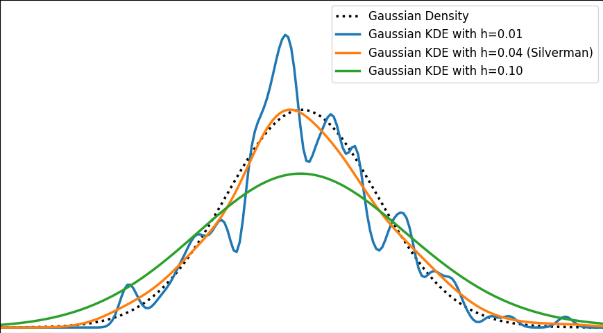
The image below depicts a Gaussian distribution being estimated by a gaussian KDE at different bandwidth values. As we can see, Silverman’s rule of thumb is well-suited, but higher bandwidths cause over-smoothing, while lower ones introduce high-frequency oscillations around the true density.
Gaussian Kernel Density Estimation from 100 samples drawn from a true gaussian distribution, for different bandwith parameters (0.01, 0.04, 0.10) — Image by the author
Examples
The video below illustrates the convergence of a Kernel Density Estimation with a Gaussian kernel across 4 standard density distributions as the number of provided samples increases.
Although it’s not optimal, I’ve chosen to keep a small constant bandwidth h over the video to better illustrate the process of kernel averaging, and to prevent excessive smoothing when the sample size is very small.
Convergence of Gaussian Kernel Density Estimation across 4 Standard Density Distributions (Uniform, Triangular, Gaussian, Gaussian Mixture) with Increasing Sample Size. — Video by the author
Implementation of Gaussian Kernel Density Estimation
Great python libraries like scipy and scikit-learn provide public implementations for Kernel Density Estimation:
scipy.stats.gaussian_kde
sklearn.neighbors.KernelDensity
However, it’s valuable to note that a basic equivalent can be built in just three lines using numpy. We need the samples x_data drawn from the distribution to estimate and the points x_prediction at which we want to evaluate the density estimate. Then, using array broadcasting we can evaluate a local gaussian kernel around each input sample and average them into the final density estimate.
N.B. This version is fast because it’s vectorized. However it involves creating a large 2D temporary array of shape (len(x_data), len(x_prediction)) to store all the kernel evaluations. To have a lower memory footprint, we could re-write it using numba or cython (to avoid the computational burden of Python for loops) to aggregate kernel evaluations on-the-fly in a running sum for each output prediction.
Real-life data is often bounded by a given domain. For example, attributes such as age, weight, or duration are always non-negative values. In such scenarios, a standard smooth KDE may fail to accurately capture the true shape of the distribution, especially if there’s a density discontinuity at the boundary.
In 1D, with the exception of some exotic cases, bounded distributions typically have either one-sided (e.g. positive values) or two-sided (e.g. uniform interval) bounded domains.
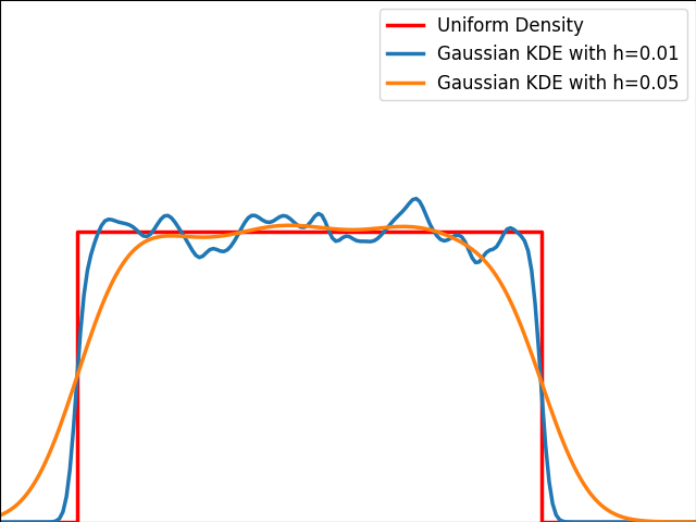
As illustrated in the graph below, kernels are bad at estimating the edges of the uniform distribution and leak outside the bounded domain.
Gaussian KDE on 100 samples drawn from a uniform distribution — Image by the author
No Clean Public Solution in Python
Unfortunately, popular public Python libraries like scipy and scikit-learn do not currently address this issue. There are existing GitHub issues and pull requests discussing this topic, but regrettably, they have remained unresolved for quite some time.
In R, kde.boundary allows Kernel density estimate for bounded data.
There are various ways to take into account the bounded nature of the distribution. Let’s describe the most popular ones: Reflection, Weighting and Transformation.
Warning: For the sake of readability, we will focus on the unit bounded domain, i.e. [0,1]. Please remember to standardize the data and scale the density appropriately in the general case [a,b].
Solution: Reflection
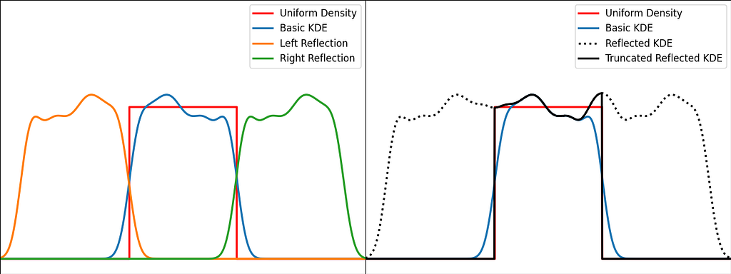
The trick is to augment the set of samples by reflecting them across the left and right boundaries. This is equivalent to reflecting the tails of the local kernels to keep them in the bounded domain. It works best when the density derivative is zero at the boundary.
The reflection technique also implies processing three times more sample points.
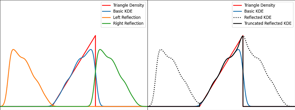
The graphs below illustrate the reflection trick for three standard distributions: uniform, right triangle and inverse square root. It does a pretty good job at reducing the bias at the boundaries, even for the singularity of the inverse square root distribution.
KDE on an uniform distribution, using reflections to handle boundaries— Image by the authorKDE on a triangle distribution, using reflections to handle boundaries — Image by the authorKDE on an inverse square root distribution, using reflections to handle boundaries — Image by the author
N.B. The signature of basic_kde has been slightly updated to allow to optionally provide your own bandwidth parameter instead of using the Silverman’s rule of thumb.
Solution: Weighting
The reflection trick presented above takes the leaking tails of the local kernel and add them back to the bounded domain, so that the information isn’t lost. However, we could also compute how much of our local kernel has been lost outside the bounded domain and leverage it to correct the bias.
For a very large number of samples, the KDE converges to the convolution between the kernel and the true density, truncated by the bounded domain.
If x is at a boundary, then only half of the kernel area will actually be used. Intuitively, we’d like to normalize the convolution kernel to make it integrate to 1 over the bounded domain. The integral will be close to 1 at the center of the bounded interval and will fall off to 0.5 near the borders. This accounts for the lack of neighboring kernels at the boundaries.
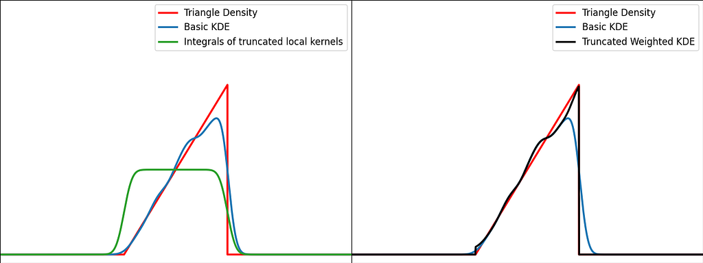
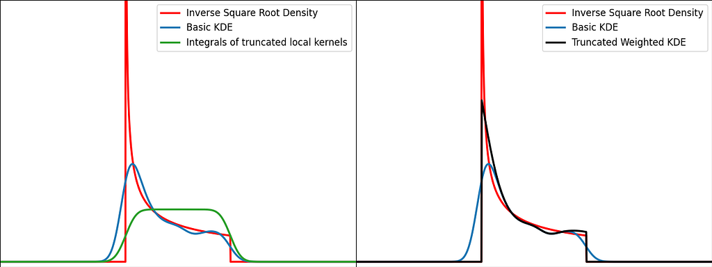
Similarly to the reflection technique, the graphs below illustrate the weighting trick for three standard distributions: uniform, right triangle and inverse square root. It performs very similarly to the reflection method.
From a computational perspective, it doesn’t require to process 3 times more samples, but it needs to evaluate the normal Cumulative Density Function at the prediction points.
KDE on an uniform distribution, applying weight on the sides to handle boundaries — Image by the authorKDE on a triangular distribution, applying weight on the sides to handle boundaries — Image by the authorKDE on an inverse square root distribution, applying weight on the sides to handle boundaries — Image by the author
Transformation
The transformation trick maps the bounded data to an unbounded space, where the KDE can be safely applied. This results in using a different kernel function for each input sample.
The logit function leverages the logarithm to map the unit interval [0,1] to the entire real axis.
Logit function — Image by the author
When applying a transform f onto a random variable X, the resulting density can be obtained by dividing by the absolute value of the derivative of f.
We can now apply it for the special case of the logit transform to retrieve the density distribution from the one estimated in the logit space.
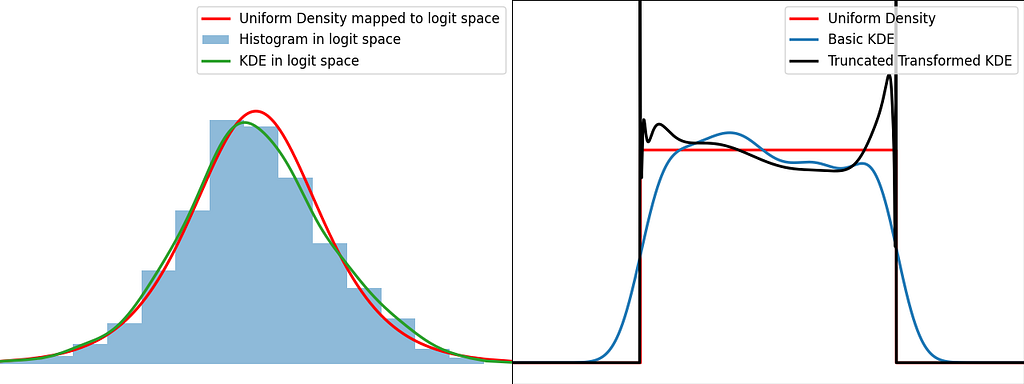
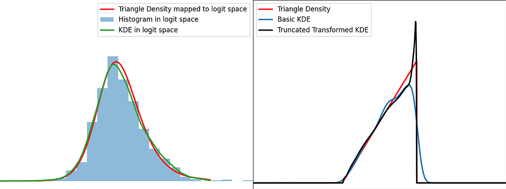
Similarly to the reflection and weighting techniques, the graphs below illustrate the weighting trick for three standard distributions: uniform, right triangle and inverse square root. It performs quite poorly by creating large oscillations at the boundaries. However, it handles extremely well the singularity of the inverse square root.
KDE on an uniform distribution, computed after mapping the samples to the logit space — Image by the authorKDE on a triangular distribution, computed after mapping the samples to the logit space — Image by the authorKDE on an inverse square root distribution, computed after mapping the samples to the logit space— Image by the authorPhoto by Martin Martz on Unsplash
Conclusion
Histograms and KDE
In Kernel Density Estimation, each sample is assigned its own local kernel density centered around it, and then we average all these densities to obtain the global density. The bandwidth parameter defines how far the influence of each kernel extends. Intuitively, we should decrease the bandwidth as the number of samples increases, to prevent excessive smoothing.
Histograms can be seen as a simplified version of KDE. Indeed, the bins implicitly define a finite set of possible rectangular kernels, and each sample is assigned to the closest one. Finally, the average of all these densities result in a piecewise-constant estimate of the global density.
Which method is the best ?
Reflection, weighting and transform are efficient basic methods to handle bounded data during KDE. However, bear in mind that there isn’t a one-size-fits-all solution; it heavily depends on the shape of your data.
The transform method handles pretty well the singularities, as we’ve seen with the inverse square root distribution. As for reflection and weighting, they are generally more suitable for a broader range of scenarios.
Reflection introduces complexity during training, whereas weighting adds complexity during inference.
From [0,1] to [a,b], [a, +∞[ and ]-∞,b]
Code presented above has been written for data bounded in the unit interval. Don’t forget to scale the density, when applying the affine transformation to normalize your data.
It can also easily be adjusted for a one-sided bounded domain, by reflecting only on one side, integrating the kernel to infinity on one side or using the logarithm instead of logit.
I hope you enjoyed reading this article and that it gave you more insights on how Kernel Density Estimation works and how to handle bounded domains!
We use cookies on our website to give you the most relevant experience by remembering your preferences and repeat visits. By clicking “Accept”, you consent to the use of ALL the cookies.
This website uses cookies to improve your experience while you navigate through the website. Out of these, the cookies that are categorized as necessary are stored on your browser as they are essential for the working of basic functionalities of the website. We also use third-party cookies that help us analyze and understand how you use this website. These cookies will be stored in your browser only with your consent. You also have the option to opt-out of these cookies. But opting out of some of these cookies may affect your browsing experience.
Necessary cookies are absolutely essential for the website to function properly. These cookies ensure basic functionalities and security features of the website, anonymously.
Cookie
Duration
Description
cookielawinfo-checkbox-analytics
11 months
This cookie is set by GDPR Cookie Consent plugin. The cookie is used to store the user consent for the cookies in the category "Analytics".
cookielawinfo-checkbox-functional
11 months
The cookie is set by GDPR cookie consent to record the user consent for the cookies in the category "Functional".
cookielawinfo-checkbox-necessary
11 months
This cookie is set by GDPR Cookie Consent plugin. The cookies is used to store the user consent for the cookies in the category "Necessary".
cookielawinfo-checkbox-others
11 months
This cookie is set by GDPR Cookie Consent plugin. The cookie is used to store the user consent for the cookies in the category "Other.
cookielawinfo-checkbox-performance
11 months
This cookie is set by GDPR Cookie Consent plugin. The cookie is used to store the user consent for the cookies in the category "Performance".
viewed_cookie_policy
11 months
The cookie is set by the GDPR Cookie Consent plugin and is used to store whether or not user has consented to the use of cookies. It does not store any personal data.
Functional cookies help to perform certain functionalities like sharing the content of the website on social media platforms, collect feedbacks, and other third-party features.
Performance cookies are used to understand and analyze the key performance indexes of the website which helps in delivering a better user experience for the visitors.
Analytical cookies are used to understand how visitors interact with the website. These cookies help provide information on metrics the number of visitors, bounce rate, traffic source, etc.
Advertisement cookies are used to provide visitors with relevant ads and marketing campaigns. These cookies track visitors across websites and collect information to provide customized ads.