Category: AI

  • End to End AI Use Case-Driven System Design

    Liz Li

    A thorough list of Technologies for best Performance/Watt

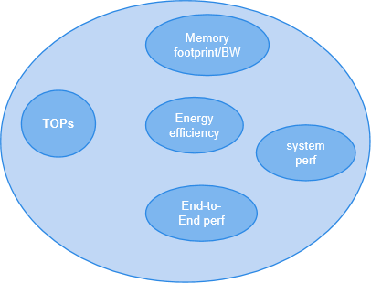
    The most commonly used metric to define AI performance is TOPs (Tera Operations Per Second), which indicates compute capability but oversimplifies the complexity of AI systems. When it comes to real AI use case system design, many other factors should also be considered beyond TOPs, including memory/cache size and bandwidth, data types, energy efficiency, etc.

    Moreover, each AI use case has its characteristics and requires a holistic examination of the whole use case pipeline. This examination delves into its impact on system components and explores optimization techniques to predict the best pipeline performance.

    Image by author

    In this post, we pick one AI use case — an end-to-end real-time infinite zoom feature with a stable diffusion-v2 inpainting model and study how to build a corresponding AI system with the best performance/Watt. This can serve as a proposal, with both well-established technologies and new research ideas that can lead to potential architectural features.

    Background on end-to-end video zoom

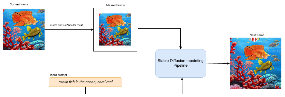
    • As shown in the below diagram, to zoom out video frames (fish image), we resize and apply a border mask to the frames before feeding them into the stable diffusion inpainting pipeline. Alongside an input text prompt, this pipeline generates frames with new content to fill the border-masked region. This process is continuously applied to each frame to achieve the continuous zoom-out effect. To conserve compute power, we may sparsely sample video frames to avoid inpainting every frame(e.g., generating 1 frame every 5 frames) if it still delivers a satisfactory user experience.
    Frame generation. Source: Infinite Zoom Stable Diffusion v2 and OpenVINO™ [1]
    • Stable diffusion-v2 inpainting pipeline is pre-trained on stable diffusion-2 model, which is a text-to-image latent diffusion model created by stability AI and LAION. The blue box in below diagram displays each function block in the inpainting pipeline
    Inpainting pipeline (inputs include text prompt, masked image and input random noise). Source: Infinite Zoom Stable Diffusion v2 and OpenVINO™ [1]
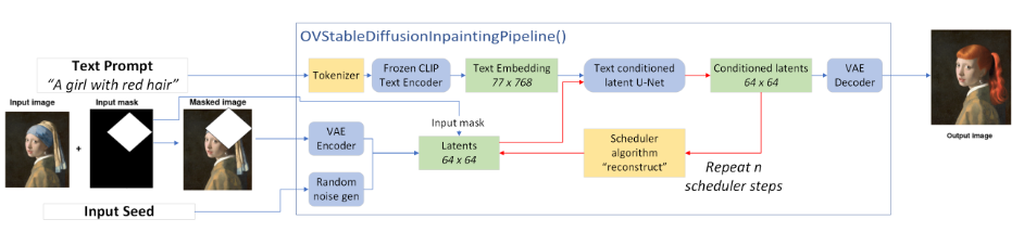
    • Stable diffusion-2 model generates 768*768 resolution images, it is trained to denoise random noise iteratively (50 steps) to get a new image. The denoising process is implemented by Unet and scheduler which is a very slow process and requires lots of compute and memory.
    Stable diffusion-2-base model. Source: The Illustrated Stable Diffusion [2]

    There are 4 models used in the pipeline as below:

    1. VAE (image encoder). Convert image into low dimensional latent representation (64*64)
    2. CLIP (text encoder). Transformer architecture (77*768), 85MP
    3. UNet (diffusion process). Iteratively denoising processing via a schedular algorithm, 865M
    4. VAE (image decoder). Transforms the latent representation back into an image (512*512)

    Most stable Diffusion operations (98% of the autoencoder and text encoder models and 84% of the U-Net) are convolutions. The bulk of the remaining U-Net operations (16%) are dense matrix multiplications due to the self-attention blocks. These models can be pretty big (varies with different hyperparameters) which requires lots of memory, for mobile devices with limited memory, it is essential to explore model compression techniques to reduce the model size, including quantization (2–4x mode size reduction and 2-3x speedup from FP16 to INT4), pruning, sparsity, etc.

    Power efficiency optimization for AI features like end-to-end video zoom

    For AI features like video zoom, power efficiency is one of the top factors for successful deployment on edge/mobile devices. These battery-operated edge devices store their energy in the battery, with the capacity of mW-H (milliWatt Hours, 1200WH means 1200 watts in one hour before it discharge, if an application is consuming 2w in one hour, then the battery can power the device for 600h). Power efficiency is computed as IPS/Watt where IPS is inferences per second (FPS/Watt for image-based applications, TOPS/Watt )

    It’s critical to reduce power consumption to get long battery life for mobile devices, there are lots of factors contributing to high power usage, including large amounts of memory transactions due to big model size, heavy computation of matrix multiplications, etc., let’s take a look at how to optimize the use case for efficient power usage.

    1. Model optimization.

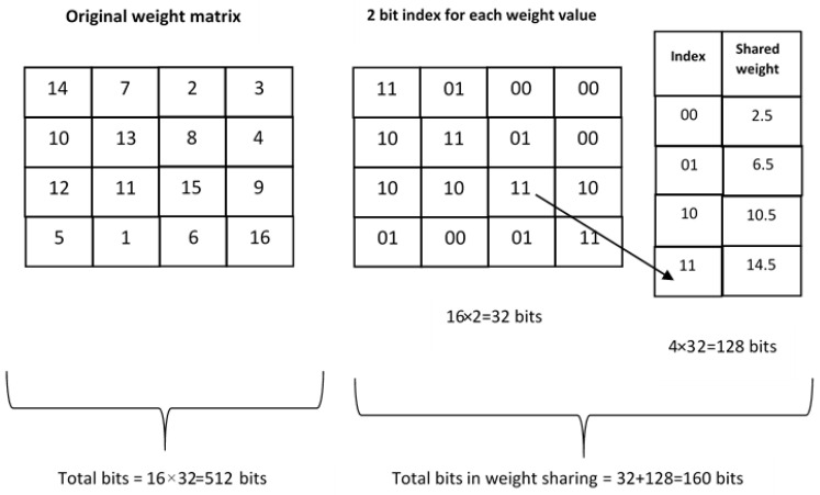
    Beyond quantization, pruning, and sparsity, there is also weight sharing. There are lots of redundant weights in the network while only a small number of weights are useful, the number of weights can be reduced by letting multiple connections share the same weight shown as below. the original 4*4 weight matrix is reduced to 4 shared weights and a 2-bit matrix, total bits are reduced from 512 bits to 160 bits.

    Weight sharing. Source: A Survey on Optimization Techniques for Edge Artificial Intelligence (AI) [3]

    2. Memory optimization.

    Memory is a critical component that consumes more power compared to matrix multiplications. For instance, the power consumption of a DRAM operation can be orders of magnitude more than that of a multiplication operation. In mobile devices, accommodating large models within local device memory is often challenging. This leads to numerous memory transactions between local device memory and DRAM, resulting in higher latency and increased energy consumption.

    Optimizing off-chip memory access is crucial for enhancing energy efficiency. The article (Optimizing Off-Chip Memory Access for Deep Neural Network Accelerator [4]) introduced an adaptive scheduling algorithm designed to minimize DRAM access. This approach demonstrated a substantial energy consumption and latency reduction, ranging between 34% and 93%.

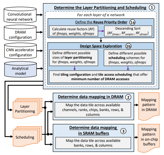
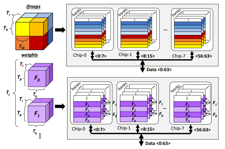
    A new method (ROMANet [5]) is proposed to minimize memory access for power saving. The core idea is to optimize the right block size of CNN layer partition to match DRAM/SRAM resources and maximize data reuse, and also optimize the tile access scheduling to minimize the number of DRAM access. The data mapping to DRAM focuses on mapping a data tile to different columns in the same row to maximize row buffer hits. For larger data tiles, same bank in different chips can be utilized for chip-level parallelism. Furthermore, if the same row in all chips is filled, data are mapped in the different banks in the same chip for bank-level parallelism. For SRAM, a similar concept of bank-level parallelism can be applied. The proposed optimization flow can save energy by 12% for the AlexNet, by 36% for the VGG-16, and by 46% for the MobileNet. A high-level flow chart of the proposed method and schematic illustration of DRAM data mapping is shown below.

    Operation flow of proposed method. Source: ROMANet [5]
    DRAM data mapping across banks and chips. Source: ROMANet [5]

    3. Dynamic power scaling.

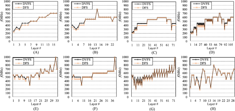
    The power of a system can be calculated by P=C*F*V², where F is the operating frequency and V is the operating voltage. Techniques like DVFS (dynamic voltage frequency scaling) was developed to optimize runtime power. It scales voltage and frequency depending on workload capacity. In deep learning, layer-wise DVFS is not appropriate as voltage scaling has long latency. On the other hand, frequency scaling is fast enough to keep up with each layer. A layer-wise dynamic frequency scaling (DFS)[6] technique is proposed for NPU, with a power model to predict power consumption to determine the highest allowable frequency. It’s demonstrated that DFS improves latency by 33%, and saves energy by 14%

    Frequency changes over layer across 8 different NN applications. Source: A layer-wise frequency scaling for a neural processing unit [6]

    4. Dedicated low-power AI HW accelerator architecture. To accelerate deep learning inference, specialized AI accelerators have shown superior power efficiency, achieving similar performance with reduced power consumption. For instance, Google’s TPU is tailored for accelerating matrix multiplication by reusing input data multiple times for computations, unlike CPUs that fetch data for each computation. This approach conserves power and diminishes data transfer latency.

    At the end

    AI inferencing is only a part of the End-to-end use case flow, there are other sub-domains to be considered while optimizing system power and performance, including imaging, codec, memory, display, graphics, etc. Breakdown of the process and examine the impact on each sub-domain is essential. for example, to look at power consumption when we run infinite zoom, we need also to look into the power of camera capturing and video processing system, display, memory, etc. make sure the power budget for each component is optimized. There are numerous optimization methods and we need to prioritize based on the use case and product

    Reference

    [1] OpenVINO tutorial: Infinite Zoom Stable Diffusion v2 and OpenVINO™

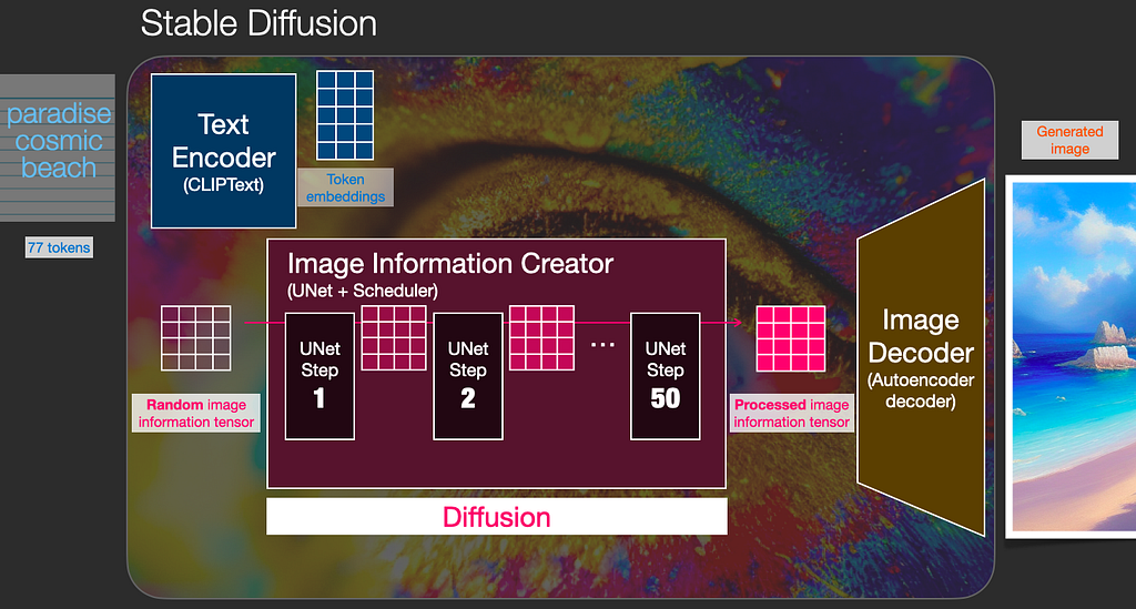
    [2] Jay Alammar, The Illustrated Stable Diffusion

    [3] Chellammal Surianarayanan et al., A Survey on Optimization Techniques for Edge Artificial Intelligence (AI), Jan 2023

    [4] Yong Zheng et al., Optimizing Off-Chip Memory Access for Deep Neural Network Accelerator, IEEE Transactions on Circuits and Systems II: Express Briefs, Volume: 69, Issue: 4, April 2022

    [5] Rachmad Vidya Wicaksana Putra et al., ROMANet: Fine grained reuse-driven off-chip memory access management and data organization for deep neural network accelerators, arxiv, 2020

    [6] Jaehoon Chung et al., A layer-wise frequency scaling for a neural processing unit, ETRI Journal, Volume 44, Issue 5, Sept 2022


    End to End AI Use Case-Driven System Design was originally published in Towards Data Science on Medium, where people are continuing the conversation by highlighting and responding to this story.

    Originally appeared here:
    End to End AI Use Case-Driven System Design

    Go Here to Read this Fast! End to End AI Use Case-Driven System Design

  • Why and How to Achieve Longer Context Windows for LLMs

    Why and How to Achieve Longer Context Windows for LLMs

    Davide Ghilardi

    Language models (LLMs) have revolutionized the field of natural language processing (NLP) over the last few years, achieving state-of-the-art results on a wide range of tasks. However, a key challenge in developing and improving these models lies in extending the length of their context. This is very important since it determines how much information is available to the model when generating an output.

    However, increasing the context window of a LLM isn’t so simple. In fact, it comes at the cost of increased computational complexity, since the attention matrix grows quadratically.

    One solution could be training the model on a large amount of data on a relatively small window (e.g. 4K tokens) and then fine-tuning it on a bigger one (e.g. 64K tokens). This operation isn’t straightforward, because even though the context length doesn’t impact the number of model’s weights, it does affect how positional information of tokens is encoded by those weights in the tokens’ dense representation.

    This reduces the model’s capacity to adapt to longer context windows even after fine-tuning, resulting in poor performance and thus requiring new techniques to encode positional information correctly and dynamically between training and fine-tuning.

    Absolute positional encoding

    In transformers, the information about the position of each token is encoded before the token is fed to the attention heads. It’s a crucial step since transformers, differently from RNNs, don’t keep track of the tokens’ position.

    The original transformer architecture [1] encodes positions as vectors of the same shape of tokens’ embeddings so that they can be added together. In particular, they used a combination of cos/sin waves with lengths increasing from low to higher order dimensions of the embedding.

    Image by author

    This method allows an efficient unique dense representation of all the tokens’ positions. However, it doesn’t solve the challenge of extending context length since these representations can’t efficiently encode relative positions of tokens.

    To see why this happens, let’s focus on a single couple of two consecutive dimensions. If we plot them on a chart, we can represent token and position embeddings as 2D vectors, as shown in the following figure:

    Image by author

    The figure above includes two charts: on the left, we have the embedding space, and on the right, there’s the key/query space. Embedding vectors are the black ones, positional vectors are the blue ones, and their sum is coloured in green.

    To shift from embeddings to keys (K) and queries (Q), the transformer applies some linear transformations defined by the two matrices Wq and Wk. Thanks to the linearity property, the transformation can be applied separately between embeddings and positional vectors. In the KQ-space the attention is computed as the dot product between keys and queries, and in the figure, it’s represented by the yellow area between the two green vectors.

    The relative distance between tokens is not directly accessible to the model since rotations mix up differently based on the original orientations of the tokens’ and positions’ embeddings, and on how they’re scaled in the transformations.

    It’s also important to note that, in this case, the addition is applied before the transformation and not vice-versa since position embeddings have to be scaled by the linear layer.

    Relative positional encoding

    To efficiently encode relative position information among tokens other methods have been proposed. We will focus on RoPE [2], which stands for Rotary Position Embedding, and for which extensions for longer context windows have been proposed.

    The two main innovations of RoPE are:

    • With RoPE, we can make the dot product between keys and queries embeddings sensitive only to the relative distance between them.
    • Positional embeddings are multiplied by the tokens’ embeddings without the need for a fixed-size look-up table.

    To achieve this goal, first, we map tokens’ embeddings from the real D-dimensional space to a complex D/2-dimensional one and apply the rotation in that space.

    Again, let’s consider a single couple of two consecutive dimensions. If we plot them on the complex plane (setting the first on the real axis and the second on the imaginary one), we can represent token embeddings as complex vectors, as shown in the following figure:

    Image by author

    Here positional encodings acquire a new meaning, in fact, they become rotations directly applied to the vectors. This change allows them to both uniquely encode the position of the token, and be preserved in the linear transformation.

    This last property is fundamental to incorporate the relative positions in the computation of attention. In fact, if we consider the attentions between the unrotated (in black) and rotated (in green) versions of kₙ and qₙ₊ₖ, represented respectively by the orange and yellow angles in the right chart, we can note something interesting:

    Image by author

    The attention between the rotated keys and queries differs from the unrotated version only by a factor proportional to the difference between their positions!

    This new property allows models trained with RoPE to show rapid convergence and lower losses and lies at the heart of some popular techniques to extend the context window beyond the training set.

    Until now we have always kept embedding dimensions fixed, but to see the whole framework, it’s also important to observe what happens along that direction.

    Image by author

    The RoPE formula defines the angle of rotation for the d-th dimension proportional to exp(-d) so, as we can see in the figure above, as d grows, the rotation applied to the embedding vector decreases exponentially (for fixed values of n and position). This feature of RoPE lets the model shift the type of information encoded in the embeddings from low-frequency (close tokens associations) to high-frequency (far tokens associations) by going from low to higher dimensions.

    RoPE extensions

    Once we have efficiently incorporated relative position information inside our model, the most straightforward way to increase the context window L of our LLM is by fine-tuning with position interpolation (PI) [3].

    It is a simple technique that scales tokens’ position to fit the new context length. So, for example, if we decide to double it, all positions will be divided in half. In particular, for any context length L* > L we want to achieve, we can define a scale factor s = L/ L* < 1.

    Although this technique has shown promising results by successfully extending the context of LLM with fine-tuning on a relatively small amount of tokens, it has its own drawbacks.

    One of them is that it slightly decreases performance (e.g. perplexity increases) for short context sizes after fine-tuning on larger ones. This issue happens because by scaling by s < 1 the position of tokens (and so also their relative distances), we reduce the rotation applied to the vectors, causing the loss of high-frequency information. Thus, the model is less able to recognize small rotations and so to figure out the positional order of close-by tokens.

    To solve this problem, we can apply a clever mechanism called NTK-aware [4] positional interpolation that instead of scaling every dimension of RoPE equally by s, spreads out the interpolation pressure across multiple dimensions by scaling high frequencies less and low frequencies more.

    Other PI extensions exist such as the NTK-by-parts [5] and dynamic NTK [6] methods. The first imposes two thresholds to limit the scaling above and below certain dimensions; the second dynamically adjusts s during inference.

    Finally, since it was observed that as the number of tokens increases, the attention softmax distribution becomes more and more “spikier” (the average entropy of attention softmax decreases), YaRN [7] (Yet another RoPE extensioN method) is a method that inverts this process by multiplying the attention matrix by a temperature factor t before the application of the softmax.

    Here’s a look at what these methods do from both position (numbers of rotations) and dimension (degree per single rotation) perspectives.

    Image by author

    Other methods

    Finally, as we said before, other context extension methods exist, here’s a brief description of the most popular ones and how they operate:

    • Alibi [8]: It’s another method for positional encoding which penalizes the attention value that that query can assign to the key depending on how far away the key and query are.
    • XPos [9]: Again another positional encoding method that generalizes RoPE to include a scaling factor.

    References

    1. Vaswani et al, 2017. Attention Is All You Need. link
    2. Su et al, 2022. RoFormer: Enhanced transformer with rotary position embedding. link
    3. Chen et al, 2023. Extending context window of large language models via positional interpolation. link
    4. bloc97, 2023. NTK-Aware Scaled RoPE allows LLaMA models to have extended (8k+) context size without any fine-tuning and minimal perplexity degradation. link
    5. bloc97, 2023. Add NTK-Aware interpolation “by parts” correction. link
    6. emozilla, 2023. Dynamically Scaled RoPE further increases performance of long context LLaMA with zero fine-tuning. link
    7. Peng et al, 2023. YaRN: Efficient Context Window Extension of Large Language Models. link
    8. Press et al, 2022. Train Short, Test Long: Attention with linear biases enables input length extrapolation. link
    9. Sun et al, 2022. A Length-Extrapolatable Transformer. link


    Why and How to Achieve Longer Context Windows for LLMs was originally published in Towards Data Science on Medium, where people are continuing the conversation by highlighting and responding to this story.

    Originally appeared here:
    Why and How to Achieve Longer Context Windows for LLMs

    Go Here to Read this Fast! Why and How to Achieve Longer Context Windows for LLMs

  • The Ins and Outs of Working with Embeddings and Embedding Models

    TDS Editors

    Ready to zoom all the way in on a timely technical topic? We hope so, because this week’s Variable is all about the fascinating world of embeddings.

    Embeddings and embedding models are essential building blocks in the powerful AI tools we’ve seen emerge in recent years, which makes it all the more important for data science and machine learning practitioners to gain fluency in this area. Even if you’ve explored embeddings in the past, it’s never a bad idea to expand your knowledge and learn about emerging approaches and use cases.

    Our highlights this week range from the relatively high-level to the very granular, and from theoretical to extremely hands-on. Regardless of how much experience you have with embeddings, we’re certain you’ll find something here to pique your curiosity.

    Photo by Alex Hu on Unsplash

    For readers who’d like to explore other topics this week, we’re thrilled to recommend some of our recent standouts:

    Thank you for supporting the work of our authors! If you’re feeling inspired to join their ranks, why not write your first post? We’d love to read it.

    Until the next Variable,

    TDS Team


    The Ins and Outs of Working with Embeddings and Embedding Models was originally published in Towards Data Science on Medium, where people are continuing the conversation by highlighting and responding to this story.

    Originally appeared here:
    The Ins and Outs of Working with Embeddings and Embedding Models

    Go Here to Read this Fast! The Ins and Outs of Working with Embeddings and Embedding Models

  • Navigating Cost-Complexity: Mixture of Thought LLM Cascades Illuminate a Path to Efficient Large…

    Navigating Cost-Complexity: Mixture of Thought LLM Cascades Illuminate a Path to Efficient Large…

    Yuval Zukerman

    Navigating Cost-Complexity: Mixture of Thought LLM Cascades Illuminate a Path to Efficient Large Language Model Deployment

    Photo by Joshua Sortino on Unsplash

    What if I told you that you could save 60% or more off of the cost of your LLM API spending without compromising on accuracy? Surprisingly, now you can.

    Large Language Models (LLMs) are now part of our everyday lives. Companies use the technology to automate processes, improve customer experiences, build better products, save money, and more.

    Hosting your own LLMs is very challenging. They offer broad capabilities but are often expensive to run. They often require complex infrastructure and massive amounts of data. Cost and complexity are why you use prompt engineering. You may even use retrieval-augmented generation (RAG) to improve context and reduce hallucinations. With both techniques, you offload running LLMs to the likes of OpenAI, Cohere, or Google. Yet, scaling LLM adoption to new use cases, especially with the latest powerful models, can drive up a new cost that was previously unaccounted for. Weaker models may be cheaper, but can you trust them with complex questions? Now, new research shows us how to save money and get as good, sometimes better, LLM results.

    Get to Know LLM Cascades

    In the search for lower LLM costs, researchers turned to the concept of LLM Cascades. In the dark ages, before the launch of ChatGPT, a team from Google and The University of Toronto defined this term as programs that use probability calculations to get the best results using multiple LLMs.

    More recently, the FrugalGPT paper defined cascades as sending a user query to a list of LLMs, one after the other, from weaker to stronger LLMs, until the answer is good enough. FrugalGPT Cascades uses a dedicated model to determine when the answer is good enough against a quality threshold.

    A recent paper titled ‘Large Language Model Cascades With Mixture of Thought Representations for Cost-Efficient Reasoning’ from George Mason University, Microsoft, and Virginia Tech offers an alternative: a function that can determine whether the answer is good enough without fine-tuning another model.

    Mixture of Thought LLM Cascades

    Instead of using several LLMs, ‘Mixture of thought’ (MoT) reasoning uses just two — GPT 3.5 Turbo and GPT 4. The former model is regarded as the ‘weaker’ LLM, while the latter is the ‘strong’ LLM. The authors harnessed LLM ‘answer consistency’ to flag whether an LLM’s response is good enough. LLMs produce consistent answers to similar prompts when they are confident the answers are correct. Therefore, when weaker LLM answers are consistent, there is no need to call the stronger LLM. Conversely, these LLMs produce inconsistent answers when they lack confidence. That’s when you need a stronger LLM to answer the prompt. (Note: you can use a weaker/stronger LLM pair of your choice as well.)

    The prompts themselves use few-shot in-context prompting to improve LLM answer quality. Such prompts guide the LLM’s response by giving examples of similar questions and answers.

    To improve model reasoning and simplify consistency measurement, the researchers introduce a new prompting technique for reasoning tasks by ‘mixing’ two prompting techniques:

    • Chain of Thought (CoT) Prompting encourages LLMs to generate intermediate steps or reasonings before arriving at a final answer. Generating these steps helps the model improve complicated task results. It also increases answer accuracy.
    • Program of Thought (PoT) extends Chain of Thought prompting and uses the model’s output as a new input for further prompts. Prompts using this technique often request the model to answer with code instead of human language.

    The paper also introduces two methods to determine answer consistency:

    • Voting: This method samples multiple answers from LLM queries with similar prompts or by varying the response temperature option. It then measures how similar the LLM’s answers are to each other. The answer that agrees the most with all the other answers is assumed to be correct. The team also defined a flexible ‘threshold’ value that aligns answer consistency and budget constraints.
    • Verification: This approach compares the LLM’s most consistent answers across two distinct thought representations (e.g., CoT and PoT). The algorithm accepts the weaker LLM’s answer if the two prompt responses are identical.

    Since voting requires multiple prompts, it may be more suitable when a budget exists to guide the threshold number.

    The Bottom Line: Mixture of Thought Saves You Money

    Let’s look at how much money the MoT technique saves and its impact on answer accuracy.

    The researchers used the following sum to calculate prompt cost:

    • The cost of prompting the weaker model (because we may prompt it several times)
    • The cost of the answer evaluation process
    • If the evaluation process rejects the answer, we add the cost of prompting the strong model

    The results were dramatic:

    • Using MoT variants — combining voting and verification with CoT and PoT — can lead to comparable performance at 40% of the cost of solely using GPT-4.
    • In testing against the CREPE Q&A dataset, MoT outperformed GPT-4 at 47% of its cost.
    • Mixing PoT and CoT improves decision-making compared to using one of the techniques alone.
    • Increasing the threshold when using the voting method did not significantly impact quality despite the additional cost.
    • The consistency model proved itself in reliably identifying correct LLM answers. It successfully predicted when to resort to using the strong model to obtain the optimal results.

    Hosting and managing Large Language Models (LLMs) in-house comes with significant challenges. They bring complexity, high costs, and the need for extensive infrastructure and data resources. As a result, LLMs present substantial hurdles for organizations seeking to harness their broad capabilities. That may lead you to turn to hosted LLMs. Yet, this approach presents companies with unforeseen cost increases and budget challenges as they expand to new use cases. That is particularly evident when integrating the latest powerful models. To avoid that fate, you face a new dilemma: Can you trust weaker, more affordable models? Can you overcome concerns about their accuracy in handling complex questions?

    LLM Cascades with Mixture of Thought (MoT) offers two significant steps forward:

    1. Substantial cost savings over exclusively using the latest models.
    2. Demonstrable results on par with the latest models.

    This breakthrough provides organizations with a practical and efficient approach to navigating the delicate balance between the powerful capabilities of LLMs and the imperative to manage costs effectively.

    Domino Staff Software Engineer Subir Mansukhani contributed to this post.


    Navigating Cost-Complexity: Mixture of Thought LLM Cascades Illuminate a Path to Efficient Large… was originally published in Towards Data Science on Medium, where people are continuing the conversation by highlighting and responding to this story.

    Originally appeared here:
    Navigating Cost-Complexity: Mixture of Thought LLM Cascades Illuminate a Path to Efficient Large…

    Go Here to Read this Fast! Navigating Cost-Complexity: Mixture of Thought LLM Cascades Illuminate a Path to Efficient Large…

  • The Role of Data Science in Democratizing AI

    The Role of Data Science in Democratizing AI

    Lior Sidi

    In the emerging era of AI development, what should be the focal points for data science teams?

    Until recently AI models were accessible only via solutions made by data scientists or other service providers. Today, AI is being democratized and available for non-AI experts allowing them to develop their own AI-driven solutions.

    What used to take weeks or months for data science teams to collect data, annotate, fit, and deploy a model, can take a few minutes to build with simple prompts and the latest generative AI model. As AI technology progresses such is the expectation to adopt it and build smarter AI-driven products and we as AI-experts hold the responsibility in supporting it across the organization.

    We at Wix are no strangers to this transformation, since 2016 (way before ChatGPT — Nov 22) our data science team has been crafting numerous impactful AI-powered features. In recent times, with the advent of the GenAI revolution, an increasing number of roles within Wix have embraced this trend and Together, we’ve successfully rolled out numerous additional features, empowering website creation with chatbots, enriching content creation capabilities, and optimizing how agencies work.

    In our role as a data science group at Wix, we bear the responsibility for ensuring the quality and widespread acceptance of AI. Recognizing the need to actively contribute to the democratization of AI, we have identified three key roles that we must undertake and spearhead: 1. Ensuring Safety, 2. Enhancing Accessibility, and 3. Improving Accuracy.

    the three roles of data science
    The three roles of data science

    Data Science + Product teams = AI Impact

    The art of building AI models is the capability to navigate and generalize to unseen edge cases. It requires a data science practice that comprises business and data understanding that is iteratively evaluated and tuned.

    Democratization of AI to product teams (product managers, developers, analysts, UX, content writers etc.) can boost the time to ship AI-driven applications but requires collaboration with data science to come up with the right processes and techniques.

    In the SWOT diagrams below we can see how data science and product teams complement each other’s weaknesses and threats with their strengths and opportunities and eventually ship impactful, reliable, cutting edge AI-products on time.

    Product team vs Data Sciemce SWOT
    Product teams vs Data Science SWOT

    1. Ensuring AI Safty

    One of the most discussed topics these days is the safety of using AI. When focusing on product-oriented solutions there are a few areas that we have to consider.

    1. Regulation — models can make decisions that might discriminate against certain populations for example give discounts based on gender or Gender discrimination for high-paying job ads. Also, when using third-party tools such as external large language models (LLMs) company secret data or users’ Personal Identifiable Information (PII) can be leaked. Recently Nature argued that there should be a regulatory overview for applications based on LLMs.
    2. Reputation — user-facing models can have mistakes and produce bad experiences, for example, a chatbot based on LLMs can answer wrongly or not up-to-date answer or toxic racist answers or Air Canada chatbot inconsistencies.
    3. Damage — decision-making models can predict wrong answers and affect the business operation, for example, a model that predicts house pricing causes 500M $ loss.

    Data scientists understand the uncertainty of AI models and can offer different solutions to handle such risks and allow safe usage of the tech, For example:

    • Safe modeling — develop models to mitigate the risk, for example, a PII masking model and misuse detection model.
    • Evaluation at scale — Apply advanced data evaluation techniques to monitor and analyze the model’s performance and type of errors.
    • Models’ customization — working with clean annotated data, filtering out harmful and irrelevant data points, and building smaller and more customizable models.
    • Ethics research — read and apply the latest research around ethics at AI and come up with best practices.

    2. Enhancing AI Accessibility

    AI should be easy to use and available to non-AI experts to integrate into their products. Until recently the way to integrate with models was online/offline models that were developed by a data scientist, they are reliable, use-case-specific models, and their predictions are accessible.

    But their main drawback is that they are not customizable by a non-AI expert. This is why we came up with a Do-AI-Yourself (D-AI-Y) approach that allows you to build your model and then deploy them as a service on a platform.

    The goal is to build simple yet valuable models fast with little AI expertise. In case the model requires improvements and research we have a data scientist on board.

    The D-AI-Y holds the following components:

    1. Education: teach the organization about AI and how to use it properly, at Wix we have an AI ambassador program, which is a gateway of AI knowledge between the different groups at Wix and the Data Science group, where groups’ representatives are trained and updated with new AI tools and best practices in order to increase scale quality and velocity of the AI-based projects in Wix.
    2. Platform: have a way to connect to LLMs and write prompts. The platform should count for the cost and scale of the model and accessibility to internal data sources. At Wix, the data science group built an AI platform that connects different roles at Wix to models from a variety of vendors (to reduce LLM vendor lock) and other capabilities like semantic search. The platform acts as a centralized hub for everyone to use and share their models, governance, monitor and serve them in production.
    3. Best practices and tools for building simple straightforward models using prompts or dedicated models to solve a certain learning task: classification, QA bot, Recommender system, semantic search, etc.
    4. Evaluation: for each learning task we suggest a certain evaluation process and also provide data curation guidance if needed.

    For example, A company builds many Q&A models using Retrieval Augment Generation (RAG), an approach that answers questions by searching for relevant evidence that can answer the question and then augment the evidence into the LLM’s prompt so it could generate a reliable answer based on it.

    So, Instead of just connecting black boxes and hoping for the best, The data science team can come up with: 1. And educational material and lectures about the RAG topic, for example this lecture I gave about semantic search used to improve RAG. 2. Equip the platform with suitable vector DB and relevant embedder 3. guidelines for building RAG, how to retrieve the evidence and write the generation prompt 4. Guidelines and tools that will support proper evaluation of RAG just like explained in this TDS post and the RAG triad by Trulens .

    This will allow many roles in the company to build their own RAG based apps models in a reliable, accurate and scalable way.

    3. Improving AI Accuracy

    As AI becomes more and more adopted such as the expectation to build more complex, accurate, and advanced solutions. At the end of the day, there is a limit to how much a non-AI expert can improve the models’ performance as it requires a deeper understanding of how the models work.

    To make models more accurate the data science group is focusing on these types of efforts:

    1. Improve common models — customize and improve models to hold Wix knowledge and outperform the external general out-of-the-box models.
    2. Customize models — highly prioritized and challenging models that the D-AI-Y can not support. Unlike common models, here we have very use-case-specific models that require customization.
    3. Improve the D-AI-Y — as we improve our D-AI-Y platform, best practices, tools, and evaluation AI becomes more accurate, therefore we keep investing research time and effort in enhancing and identifying innovative ways to make it better.

    Conclusion

    After years of waiting, the democratization of AI is happening, let’s embrace it! Product teams’ inherent understanding of the business together with the ease of use of GenAI allows them to build AI-driven features that boost their product capabilities.

    Because non-AI experts are not equipped with a deep understanding of how AI models work and how to evaluate them properly at scale they might face issues around results’ reliability and accuracy. This is where the data science group can assist and support their efforts by guiding the teams on how to safely use the models, create mitigation services if needed, share the latest best practices around new AI capabilities, evaluate their performance, and serve them at scale.

    When an AI feature shows great business impact, the product teams will immediately start shifting their effort towards improving the results, this is where data scientists can offer advanced approaches to improve performance as they understand how these models work.

    To conclude, The role of data science in democratizing AI is a crucial one, as it bridges the gap between AI technology and those who may not have extensive AI expertise. Through collaboration between data scientists and product teams, we can harness the strengths of both fields to create safe, accessible, and accurate AI-driven solutions that drive innovation and deliver exceptional user experiences. With ongoing advancements and innovations, the future of democratized AI holds great potential for transformative change across industries.

    *Unless otherwise noted, all images are by the author


    The Role of Data Science in Democratizing AI was originally published in Towards Data Science on Medium, where people are continuing the conversation by highlighting and responding to this story.

    Originally appeared here:
    The Role of Data Science in Democratizing AI

    Go Here to Read this Fast! The Role of Data Science in Democratizing AI

  • Training CausalLM Models Part 1: What Actually Is CausalLM?

    Training CausalLM Models Part 1: What Actually Is CausalLM?

    Theo Lebryk

    The first part of a practical guide to using HuggingFace’s CausalLM class

    Causal langauge models model each new word as a function of all previous words. Source: Pexels

    If you’ve played around with recent models on HuggingFace, chances are you encountered a causal language model. When you pull up the documentation for a model family, you’ll get a page with “tasks” like LlamaForCausalLM or LlamaForSequenceClassification.

    If you’re like me, going from that documentation to actually finetuning a model can be a bit confusing. We’re going to focus on CausalLM, starting by explaining what CausalLM is in this post followed by a practical example of how to finetune a CausalLM model in a subsequent post.

    Background: Encoders and Decoders

    Many of the best models today such as LLAMA-2, GPT-2, or Falcon are “decoder-only” models. A decoder-only model:

    1. takes a sequence of previous tokens (AKA a prompt)
    2. runs those tokens through the model (often creating embeddings from tokens and running them through transformer blocks)
    3. outputs a single output (usually the probability of the next token).

    This is contrasted with models with “encoder-only” or hybrid “encoder-decoder” architectures which will input the entire sequence, not just previous tokens. This difference disposes the two architectures towards different tasks. Decoder models are designed for the generative task of writing new text. Encoder models are designed for tasks which require looking at a full sequence such as translation or sequence classification. Things get murky because you can repurpose a decoder-only model to do translation or use an encoder-only model to generate new text. Sebastian Raschka has a nice guide if you want to dig more into encoders vs decoders. There’s a also a medium article which goes more in-depth into the differeneces between masked langauge modeling and causal langauge modeling.

    For our purposes, all you need to know is that:

    1. CausalLM models generally are decoder-only models
    2. Decoder-only models look at past tokens to predict the next token

    With decoder-only language models, we can think of the next token prediction process as “causal language modeling” because the previous tokens “cause” each additional token.

    HuggingFace CausalLM

    In HuggingFace world, CausalLM (LM stands for language modeling) is a class of models which take a prompt and predict new tokens. In reality, we’re predicting one token at a time, but the class abstracts away the tediousness of having to loop through sequences one token at a time. During inference, CausalLMs will iteratively predict individual tokens until some stopping condition at which point the model returns the final concatenated tokens.

    During training, something similar happens where we give the model a sequence of tokens we want to learn. We start by predicting the second token given the first one, then the third token given the first two tokens and so on.

    Thus, if you want to learn how to predict the sentence “the dog likes food,” assuming each word is a token, you’re making 3 predictions:

    1. “the” → dog,
    2. “the dog” → likes
    3. “the dog likes” → food

    During training, you can think about each of the three snapshots of the sentence as three observations in your training dataset. Manually splitting long sequences into individual rows for each token in a sequence would be tedious, so HuggingFace handles it for you.

    As long as you give it a sequence of tokens, it will break out that sequence into individual single token predictions behind the scenes.

    You can create this ‘sequence of tokens’ by running a regular string through the model’s tokenizer. The tokenizer will output a dictionary-like object with input_ids and an attention_mask as keys, like with any ordinary HuggingFace model.

    from transformers import AutoTokenizer
    tokenizer = AutoTokenizer.from_pretrained("bigscience/bloom-560m")
    tokenizer("the dog likes food")
    >>> {'input_ids': [5984, 35433, 114022, 17304], 'attention_mask': [1, 1, 1, 1]}

    With CausalLM models, there’s one additional step where the model expects a labels key. During training, we use the “previous” input_ids to predict the “current” labels token. However, you do not want to think about labels like a question answering model where the first index of labels corresponds with the answer to the input_ids (i.e. that the labels should be concatenated to the end of the input_ids). Rather, you want labels and input_ids to mirror each other with identical shapes. In algebraic notation, to predict labels token at index k, we use all the input_ids through the k-1 index.

    If this is confusing, practically, you can usually just make labels an identical copy of input_ids and call it a day. If you do want to understand what’s going on, we’ll walk through an example.

    A quick worked example

    Let’s go back to “the dog likes food.” For simplicity, let’s leave the words as words rather than assigning them to token numbers, but in practice these would be numbers which you can map back to their true string representation using the tokenizer.

    Our input for a single element batch would look like this:

    {
    "input_ids": [["the", "dog", "likes", "food"]],
    "attention_mask": [[1, 1, 1, 1]],
    "labels": [["the", "dog", "likes", "food"]],
    }

    The double brackets denote that technically the shape for the arrays for each key is batch_size x sequence_size. To keep things simple, we can ignore batching and just treat them like one dimensional vectors.

    Under the hood, if the model is predicting the kth token in a sequence, it will do so kind of like so:

    pred_token_k = model(input_ids[:k]*attention_mask[:k]^T)

    Note this is pseudocode.

    We can ignore the attention mask for our purposes. For CausalLM models, we usually want the attention mask to be all 1s because we want to attend to all previous tokens. Also note that [:k] really means we use the 0th index through the k-1 index because the ending index in slicing is exclusive.

    With that in mind, we have:

    pred_token_k = model(input_ids[:k])

    The loss would be taken by comparing the true value of labels[k] with pred_token_k.

    In reality, both get represented as 1xv vectors where v is the size of the vocabulary. Each element represents the probability of that token. For the predictions (pred_token_k), these are real probabilities the model predicts. For the true label (labels[k]), we can artificially make it the correct shape by making a vector with 1 for the actual true token and 0 for all other tokens in the vocabulary.

    Let’s say we’re predicting the second word of our sample sentence, meaning k=1 (we’re zero indexing k). The first bullet item is the context we use to generate a prediction and the second bullet item is the true label token we’re aiming to predict.

    k=1:

    • Input_ids[:1] == [the]
    • Labels[1] == dog

    k=2:

    • Input_ids[:2] == [the, dog]
    • Labels[2] == likes

    k =3:

    • Input_ids[:3] == [the, dog, likes]
    • Labels[3] == food

    Let’s say k=3 and we feed the model “[the, dog, likes]”. The model outputs:

    [P(dog)=10%, P(food)=60%,P(likes)=0%, P(the)=30%]

    In other words, the model thinks there’s a 10% chance the next token is “dog,” 60% chance the next token is “food” and 30% chance the next token is “the.”

    The true label could be represented as:

    [P(dog)=0%, P(food)=100%, P(likes)=0%, P(the)=0%]

    In real training, we’d use a loss function like cross-entropy. To keep it as intuitive as possible, let’s just use absolute difference to get an approximate feel for loss. By absolute difference, I mean the absolute value of the difference between the predicted probability and our “true” probability: e.g. absolute_diff_dog = |0.10–0.00| = 0.10.

    Even with this crude loss function, you can see that to minimize the loss we want to predict a high probability for the actual label (e.g. food) and low probabilities for all other tokens in the vocabulary.

    For instance, let’s say after training, when we ask our model to predict the next token given [the, dog, likes], our outputs look like the following:

    Now our loss is smaller now that we’ve learned to predict “food” with high probability given those inputs.

    Training would just be repeating this process of trying to align the predicted probabilities with the true next token for all the tokens in your training sequences.

    Conclusion

    Hopefully you’re getting an intuition about what’s happening under the hood to train a CausalLM model using HuggingFace. You might have some questions like “why do we need labels as a separate array when we could just use the kth index of input_ids directly at each step? Is there any case when labels would be different than input_ids?”

    I’m going to leave you to think about those questions and stop there for now. We’ll pick back up with answers and real code in the next post!


    Training CausalLM Models Part 1: What Actually Is CausalLM? was originally published in Towards Data Science on Medium, where people are continuing the conversation by highlighting and responding to this story.

    Originally appeared here:
    Training CausalLM Models Part 1: What Actually Is CausalLM?

    Go Here to Read this Fast! Training CausalLM Models Part 1: What Actually Is CausalLM?