In this post, we illustrate how EBSCOlearning partnered with AWS Generative AI Innovation Center (GenAIIC) to use the power of generative AI in revolutionizing their learning assessment process. We explore the challenges faced in traditional question-answer (QA) generation and the innovative AI-driven solution developed to address them.
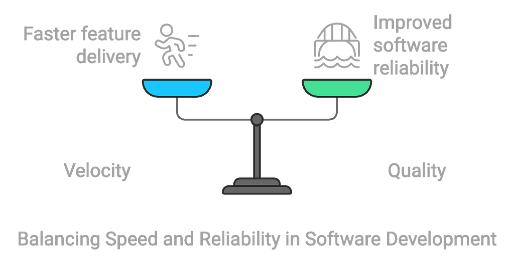
Deprioritizing quality sacrifices both software stability and velocity, leading to costly issues. Investing in quality boosts speed and outcomes.
Image by the author. (AI generated Midjourney)
Investing in software quality is often easier said than done. Although many engineering managers express a commitment to high-quality software, they are often cautious about allocating substantial resources toward quality-focused initiatives. Pressed by tight deadlines and competing priorities, leaders frequently face tough choices in how they allocate their team’s time and effort. As a result, investments in quality are often the first to be cut.
The tension between investing in quality and prioritizing velocity is pivotal in any engineering organization and especially with more cutting-edge data science and machine learning projects where delivering results is at the forefront. Unlike traditional software development, ML systems often require continuous updates to maintain model performance, adapt to changing data distributions, and integrate new features. Production issues in ML pipelines — such as data quality problems, model drift, or deployment failures — can disrupt these workflows and have cascading effects on business outcomes. Balancing the speed of experimentation and deployment with rigorous quality assurance is crucial for ML teams to deliver reliable, high-performing models. By applying a structured, scientific approach to quantify the cost of production issues, as outlined in this blog post, ML teams can make informed decisions about where to invest in quality improvements and optimize their development velocity.
Quality often faces a formidable rival: velocity. As pressure to meet business goals and deliver critical features intensifies, it becomes challenging to justify any approach that doesn’t directly drive output. Many teams reduce non-coding activities to the bare minimum, focusing on unit tests while deprioritizing integration tests, delaying technical improvements, and relying on observability tools to catch production issues — hoping to address them only if they arise.
Balancing velocity and quality is rarely a straightforward choice, and this post doesn’t aim to simplify it. However, what leaders often overlook is that velocity and quality are deeply connected. By deprioritizing initiatives that improve software quality, teams may end up with releases that are both bug-ridden and slow. Any gains from pushing more features out quickly can quickly erode, as maintenance problems and a steady influx of issues ultimately undermine the team’s velocity.
Only by understanding the full impact of quality on velocity and the expected ROI of quality initiatives can leaders make informed decisions about balancing their team’s backlog.
In this post, we will attempt to provide a model to measure the ROI of investment in two aspects of improving release quality: reducing the number of production issues, and reducing the time spent by the teams on these issues when they occur.
Escape defects, the bugs that make their way to production
Preventing regressions is probably the most direct, top-of-the-funnel measure to reduce the overhead of production issues on the team. Issues that never occurred will not weigh the team down, cause interruptions, or threaten business continuity.
As appealing as the benefits might be, there is an inflection point after which defending the code from issues can slow releases to a grinding halt. Theoretically, the team could triple the number of required code reviews, triple investment in tests, and build a rigorous load testing apparatus. It will find itself preventing more issues but also extremely slow to release any new content.
Therefore, in order to justify investing in any type of effort to prevent regressions, we need to understand the ROI better. We can try to approximate the cost saving of each 1% decrease in regressions on the overall team performance to start establishing a framework we can use to balance quality investment.
Image by the author.
The direct gain of preventing issues is first of all with the time the team spends handling these issues. Studies show teams currently spend anywhere between 20–40% of their time working on production issues — a substantial drain on productivity.
What would be the benefit of investing in preventing issues? Using simple math we can start estimating the improvement in productivity for each issue that can be prevented in earlier stages of the development process:
Image by the author.
Where:
Tsaved is the time saved through issue prevention.
Tissues is the current time spent on production issues.
P is the percentage of production issues that could be prevented.
This framework aids in assessing the cost vs. value of engineering investments. For example, a manager assigns two developers a week to analyze performance issues using observability data. Their efforts reduce production issues by 10%.
In a 100-developer team where 40% of time is spent on issue resolution, this translates to a 4% capacity gain, plus an additional 1.6% from reduced context switching. With 5.6% capacity reclaimed, the investment in two developers proves worthwhile, showing how this approach can guide practical decision-making.
It’s straightforward to see the direct impact of preventing every single 1% of production regressions on the team’s velocity. This represents work on production regressions that the team would not need to perform. The below table can give some context by plugging in a few values:
Given this data, as an example, the direct gain in team resources for each 1% improvement for a team that spends 25% of its time dealing with production issues would be 0.25%. If the team were able to prevent 20% of production issues, it would then mean 5%back to the engineering team. While this might not sound like a sizeable enough chunk, there are other costs related to issues we can try to optimize as well for an even bigger impact.
Mean Time to Resolution (MTTR): Reducing Time Lost to Issue Resolution
In the previous example, we looked at the productivity gain achieved by preventing issues. But what about those issues that can’t be avoided? While some bugs are inevitable, we can still minimize their impact on the team’s productivity by reducing the time it takes to resolve them — known as the Mean Time to Resolution (MTTR).
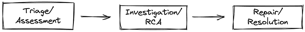
Typically, resolving a bug involves several stages:
Triage/Assessment: The team gathers relevant subject matter experts to determine the severity and urgency of the issue.
Investigation/Root Cause Analysis (RCA): Developers dig into the problem to identify the underlying cause, often the most time-consuming phase.
Repair/Resolution: The team implements the fix.
Image by the author.
Among these stages, the investigation phase often represents the greatest opportunity for time savings. By adopting more efficient tools for tracing, debugging, and defect analysis, teams can streamline their RCA efforts, significantly reducing MTTR and, in turn, boosting productivity. During triage, the team may involve subject matter experts to assess if an issue belongs in the backlog and determine its urgency. Investigation and root cause analysis (RCA) follows, where developers dig into the problem. Finally, the repair phase involves writing code to fix the issue. Interestingly, the first two phases, especially investigation and RCA, often consume 30–50% of the total resolution time. This stage holds the greatest potential for optimization, as the key is improving how existing information is analyzed.
To measure the effect of improving the investigation time on the team velocity we can take the the percentage of time the team spends on an issue and reduce the proportional cost of the investigation stage. This can usually be accomplished by adopting better tooling for tracing, debugging, and defect analysis. We apply similar logic to the issue prevention assessment in order to get an idea of how much productivity the team could gain with each percentage of reduction in investigation time.
Image by the author.
Tsaved : Percentage of team time saved
R: Reduction in investigation time
T_investigation : Time per issue spent on investigation efforts
T_issues : Percentage of time spent on production issues
We can test out what would be the performance gain relative to the T_investigationand T_issuesvariables. We will calculate the marginal gain for each percent of investigation time reduction R .
As these numbers begin to add up the team can achieve a significant gain. If we are able to improve investigation time by 40%, for example, in a team that spends 25% of its time dealing with production issues, we would be reclaiming another 4% of that team’s productivity.
Combining the two benefits
With these two areas of optimization under consideration, we can create a unified formula to measure the combined effect of optimizing both issue prevention and the time the team spends on issues it is not able to prevent.
Image by the author.
Going back to our example organization that spends 25% of the time on prod issues and 40% of the resolution time per issue on investigation, a reduction of 40% in investigation time and prevention of 20% of the issues would result in an 8.1% improvement to the team productivity. However, we are far from done.
Accounting for the hidden cost of context-switching
Each of the above naive calculations does not take into account a major penalty incurred by work being interrupted due to unplanned production issues — context switching (CS). There are numerous studies that repeatedly show that context switching is expensive. How expensive? A penalty of anywhere between 20% to 70% extra work because of interruptions and switching between several tasks. In reducing interrupted work time we can also reduce the context switching penalty.
Our original formula did not account for that important variable. A simple though naive way of doing that would be to assume that any unplanned work handling production issues incur an equivalent context-switching penalty on the backlog items already assigned to the team. If we are able to save 8% of the team velocity, that should result in an equivalent reduction of context switching working on the original planned tasks. In reducing 8% of unplanned work we have also therefore reduced the CS penalty of the equivalent 8% of planned work the team needs to complete as well.
Let’s add that to our equation:
Image by the author.
Continuing our example, our hypothetical organization would find that the actual impact of their improvements is now a little over 11%. For a dev team of 80 engineers, that would be more than 8 developers free to do something else to contribute to the backlog.
Use the ROI calculator
To make things easier, I’ve uploaded all of the above formulas as a simple HTML calculator that you can access here:
Production issues are costly, but a clear ROI framework helps quantify the impact of quality improvements. Reducing Mean Time to Resolution (MTTR) through optimized triage and investigation can boost team productivity. For example, a 40% reduction in investigation time recovers 4% of capacity and lowers the hidden cost of context-switching.
Use the ROI Calculator to evaluate quality investments and make data-driven decisions. Access it here to see how targeted improvements enhance efficiency.
Discover how DDPG solves the puzzle of continuous action control, unlocking possibilities in AI-driven medical robotics.
Imagine you’re controlling a roboticarm in a surgical procedure. Discrete actions might be:
Move up,
Move down,
Grab, or
Release
These are clear, direct commands, easy to execute in simple scenarios.
But what about performing delicate movements, such as:
Move the arm by 0.5 mm to avoid damaging the tissue,
Apply a force of 3N for tissue compression, or
Rotate the wrist by 15° to adjust the incision angle?
In these situations, you need more than just choosing an action — you must decide how much of that action is needed. This is the world of continuous action spaces, and this is where Deep Deterministic Policy Gradient (DDPG) shines!
Traditional methods like Deep Q-Networks (DQN) work well with discrete actions but struggle with continuous ones. DeterministicPolicyGradient (DPG) on the other hand, tackled this issue but faced challenges with poor exploration and instability. DDPG which wasfirst introduced in T P. Lillicrap et al’s papercombines the strengths of DPG and DQN to improve stability and performance in environments with continuous action spaces.
In this post, we will discuss the theory and architecture behind DDPG, look at an implementation of it on Python, evaluate its performance (by testing it on MountainCarContinuous game) and briefly discuss how DDPG can be used in the bioengineering field.
DDPG Architecture
Unlike DQN, which evaluates every possible state-action pair to find the best action (impossible in continuous spaces due to infinite combinations), DPG uses an Actor-Critic architecture. The Actor learns a policy that directly maps states to actions, avoiding exhaustive searches and focusing on learning the best action for each state.
However, DPG faces two main challenges:
It is a deterministic algorithm which limits exploration of the action space.
It cannot use neural networks effectively due to instability in the learning process.
DDPG improves DPG by introducing exploration noise via the Ornstein-Uhlenbeck process and stabilising training with Batch Normalisation and DQN techniques like Replay Buffer and Target Networks.
With these enhancements, DDPG is well-suited to train agents in continuous action spaces, such as controlling robotic systems in bioengineering applications.
Now, let’s explore the key components of the DDPG model!
Actor-Critic Framework
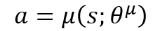
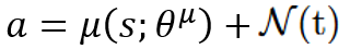
Actor (Policy Network): Tells the agent which action to take given the state it is in. The network’s parameters (i.e. weights) are represented by θμ.
Tip! Think of the Actor Network as the decision-maker: it maps the current state to a single action.
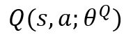
Critic (Q-value Network): Evaluates how good the action taken by the actor by estimating the Q-value of that state-action pair.
Tip! Think of the Critic Network as the evaluator, it assigns a quality score to each action and helps improve the Actor’s policy to make sure it indeed generates the best action to take in each given state.
Note! The critic will use the estimated Q-value for two things:
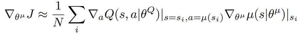
To improve the Actor’s policy (Actor Policy Update).
The Actor’s goal is to adjust its parameters (θμ) so that it outputs actions that maximise the critic’s Q-value.
To do so, the Actor needs to understand both how the selected action a affects the Critic’s Q-value and how its internal parameters affect its Policy which is done through this Policy Gradient equation (it is the mean of all the gradients calculated from the mini-batch):
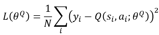
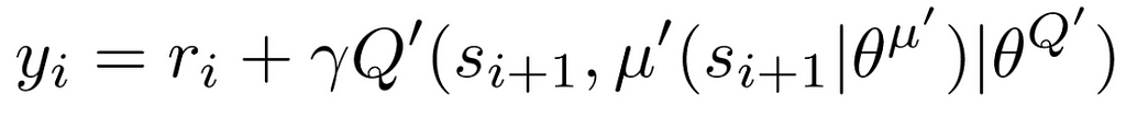
2. To improve its own network (Critic Q-value Network Update) by minimising the loss function below.
Where N is the number of experiences sampled in the mini-batch and y_i is the target Q-value calculated as follows.
Replay Buffer
As the agent explores the environment, past experiences (state, action, reward, next state) are stored as tuples (s, a, r, s′) in the replay buffer. During training, mini-batches consisting of some of these experiences are then randomly sampled to train the agent.
Question! How does replay buffer actually reduce instability?
By randomly sampling experiences, the replay buffer breaks the correlation between consecutive samples, reducing bias and leading to more stable training.
Target Networks
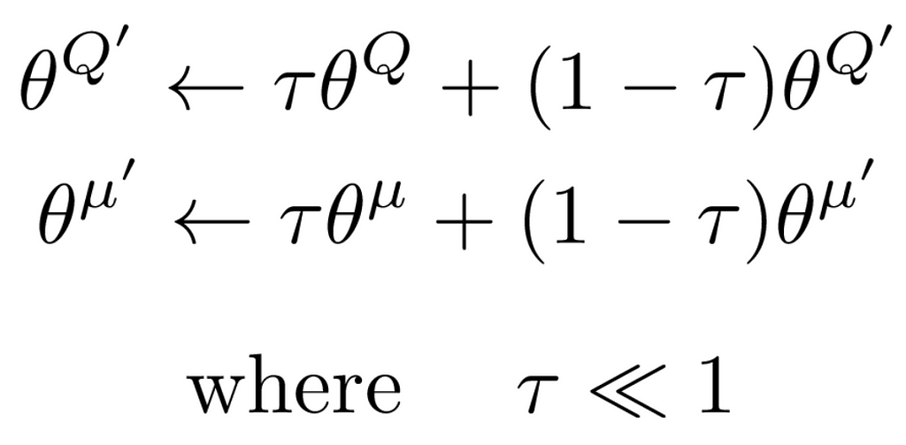
Target Networks are slowly updated copies of the Actor and Critic. They provide stable Q-value targets, preventing rapid changes and ensuring smooth, consistent updates.
Question! How do target networks actually reduce instability?
Without the Critic target network, the target Q-value is calculated directly from the Critic Q-value network, which is updated continuously. This causes the target Q-value to shift at each step, creating a “moving target” problem. As a result, the Critic ends up chasing a constantly changing target, making training unstable.
Additionally, since the Actor relies on the Critic’s feedback, errors in one network can amplify errors in the other, creating an interdependent loop of instability.
By introducing target networks that are updated gradually with a soft update rule, we ensure the target Q-value remains more consistent, reducing abrupt changes and improving learning stability.
Batch Normalisation
Batch Normalisation standardises the inputs to each layer of the neural network, ensuring mean of zero and a unit variance.
Question! How does batch normalisation actually reduce instability?
Samples drawn from the replay buffer may have different distributions than real-time data, leading to instability during network updates.
Batch normalisation ensures consistent scaling of inputs to prevent erratic updates caused by varying input distributions.
Exploration Noise
Since the Actor’s policy is deterministic, exploration noise is added to actions during training to encourage the agent to explore the as much of the action space as possible.
On the DDPG publication, the authors used the Ornstein-Uhlenbeck process to generate temporally correlated noise, in order to mimick real-world system dynamics.
class Actor(nn.Module): """ Actor network for the DDPG algorithm. """ def __init__(self, state_dim, action_dim, max_action,use_batch_norm): """ Initialise the Actor's Policy network.
:param state_dim: Dimension of the state space :param action_dim: Dimension of the action space :param max_action: Maximum value of the action """ super(Actor, self).__init__() self.bn1 = nn.LayerNorm(HIDDEN_LAYERS_ACTOR) if use_batch_norm else nn.Identity() self.bn2 = nn.LayerNorm(HIDDEN_LAYERS_ACTOR) if use_batch_norm else nn.Identity()
def forward(self, state): """ Forward propagation through the network.
:param state: Input state :return: Action """
a = torch.relu(self.bn1(self.l1(state))) a = torch.relu(self.bn2(self.l2(a))) return self.max_action * torch.tanh(self.l3(a))
class Critic(nn.Module): """ Critic network for the DDPG algorithm. """ def __init__(self, state_dim, action_dim,use_batch_norm): """ Initialise the Critic's Value network.
:param state_dim: Dimension of the state space :param action_dim: Dimension of the action space """ super(Critic, self).__init__() self.bn1 = nn.BatchNorm1d(HIDDEN_LAYERS_CRITIC) if use_batch_norm else nn.Identity() self.bn2 = nn.BatchNorm1d(HIDDEN_LAYERS_CRITIC) if use_batch_norm else nn.Identity() self.l1 = nn.Linear(state_dim + action_dim, HIDDEN_LAYERS_CRITIC)
A ReplayBuffer class is implemented to store and sample the transition tuples (s, a, r, s’) discussed in the previous section to enable mini-batch off-policy learning.
class ReplayBuffer: def __init__(self, capacity): self.buffer = deque(maxlen=capacity)
A DDPG class was defined and it encapsulates the agent’s behavior:
Initialisation: Creates Actor and Critic networks, along with their target counterparts and the replay buffer.
class DDPG():
    """
    Deep Deterministic Policy Gradient (DDPG) agent.
    """
    def __init__(self, state_dim, action_dim, max_action,use_batch_norm):
        """
        Initialise the DDPG agent.

        :param state_dim: Dimension of the state space
        :param action_dim: Dimension of the action space
        :param max_action: Maximum value of the action
        """
        # [STEP 0]
        # Initialise Actor's Policy network
        self.actor = Actor(state_dim, action_dim, max_action,use_batch_norm)
        # Initialise Actor target network with same weights as Actor's Policy network
        self.actor_target = Actor(state_dim, action_dim, max_action,use_batch_norm)
        self.actor_target.load_state_dict(self.actor.state_dict())
        self.actor_optimizer = optim.Adam(self.actor.parameters(), lr=ACTOR_LR)

        # Initialise Critic's Value network
        self.critic = Critic(state_dim, action_dim,use_batch_norm)
        # Initialise Crtic's target network with same weights as Critic's Value network
        self.critic_target = Critic(state_dim, action_dim,use_batch_norm)
        self.critic_target.load_state_dict(self.critic.state_dict())
        self.critic_optimizer = optim.Adam(self.critic.parameters(), lr=CRITIC_LR)

        # Initialise the Replay Buffer
        self.replay_buffer = ReplayBuffer(BUFFER_SIZE)
2. Action Selection: The select_action method chooses actions based on the current policy.
    def select_action(self, state):
        """
        Select an action given the current state.

        :param state: Current state
        :return: Selected action
        """
        state = torch.FloatTensor(state.reshape(1, -1))
        action = self.actor(state).cpu().data.numpy().flatten()
        return action
3. Training: The train method defines how the networks are updated using experiences from the replay buffer.
Note! Since the paper introduced the use of target networks and batch normalisation to improve stability, I designed the train method to allow us to toggle these methods on or off. This lets us compare the agent’s performance with and without them. See code below for exact implementation.
def train(self, use_target_network,use_batch_norm): """ Train the DDPG agent.
:param use_target_network: Whether to use target networks or not :param use_batch_norm: Whether to use batch normalisation or not """ if len(self.replay_buffer) < BATCH_SIZE: return
# [STEP 4]. Sample a batch from the replay buffer batch = self.replay_buffer.sample(BATCH_SIZE) state, action, reward, next_state, done = map(np.stack, zip(*batch))
# [STEP 6]. Use gradient descent to update weights of the Critic network # to minimise loss function self.critic_optimizer.zero_grad() critic_loss.backward() self.critic_optimizer.step()
# Actor Network update # actor_loss = -self.critic(state, self.actor(state)).mean()
# [STEP 7]. Use gradient descent to update weights of the Actor network # to minimise loss function and maximise the Q-value => choose the action that yields the highest cumulative reward self.actor_optimizer.zero_grad() actor_loss.backward() self.actor_optimizer.step()
# [STEP 8]. Update target networks if use_target_network: for param, target_param in zip(self.critic.parameters(), self.critic_target.parameters()): target_param.data.copy_(TAU * param.data + (1 - TAU) * target_param.data)
for param, target_param in zip(self.actor.parameters(), self.actor_target.parameters()): target_param.data.copy_(TAU * param.data + (1 - TAU) * target_param.data)
Train the DDPG agent
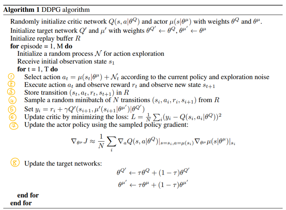
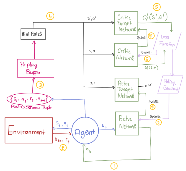
Bringing all the defined classes and methods together, we can train the DDPG agent. My train_dppg function follows the pseudocode and DDPG model diagram structure.
Tip: To make it easier for you to understand, I’ve labeled each code section with the corresponding step number from both the pseudocode and diagram. Hope that helps! 🙂
def train_ddpg(use_target_network, use_batch_norm, num_episodes=NUM_EPISODES): """ Train the DDPG agent.
:param use_target_network: Whether to use target networks :param use_batch_norm: Whether to use batch normalization :param num_episodes: Number of episodes to train :return: List of episode rewards """ agent = DDPG(state_dim, action_dim, 1,use_batch_norm)
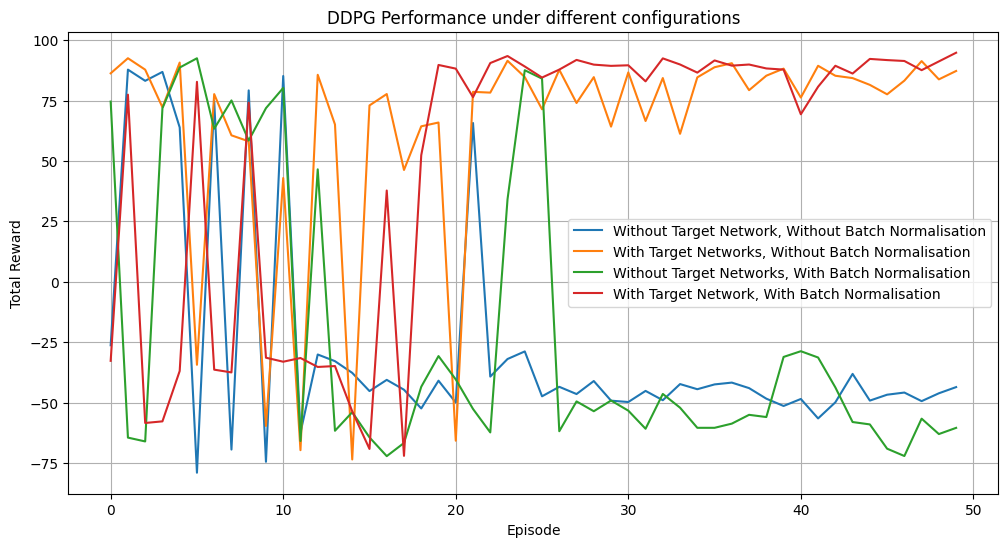
Performance and Results: Evaluating DDPG’s Effectiveness
DDPG’s effectiveness in a continuous action space was tested in the MountainCarContinuous-v0 environment, where the agent learns to where the agent learns to gain momentum to drive the car up a steep hill. The results show that using Target Networks and Batch Normalisation leads to faster convergence, higher rewards, and more stable learning than other configurations.
Graph generated by authorGIF generated by author
Note! You can implement this yourself on any environment of your choice by running the code which can be found on my GitHub as is and simply changing the environment’s name as needed!
DDPG in Bioengineering: Unlocking Precision and Adaptability
Through this blog post, we’ve seen that DDPG is a powerful algorithm for training agents in environments with continuous action spaces. By combining techniques from both DPG and DQN, DDPG improves exploration, stability, and performance — key factors for applications in robotic surgery and bioengineering.
Imagine a robotic surgeon, like the da Vinci system, using DDPG to control fine movements in real-time, ensuring precise adjustments without any errors. With DDPG, the robot could adjust its arm’s position by millimeters, apply exact force when suturing, or even make slight wrist rotations for an optimal incision. Such real-time precision could transform surgical outcomes, reduce recovery time, and minimise human error.
But DDPG’s potential goes beyond surgery. It’s already advancing bioengineering, enabling robotic prosthetics and assistive devices to replicate the natural motion of human limbs (check out this super interesting article!).
Now that we’ve covered the theory behind DDPG, it’s time for you to explore its implementation. Start with simple examples and gradually dive into more complex scenarios!
References
Lillicrap TP, Hunt JJ, Pritzel A, Heess N, Erez T, Tassa Y, et al. Continuous control with deep reinforcement learning [Internet]. arXiv; 2019. Available from: http://arxiv.org/abs/1509.02971
Disclosure: I am a maintainer of Opik, one of the open source projects used later in this article.
For the past few months, I’ve been working on LLM-based evaluations (“LLM-as-a-Judge” metrics) for language models. The results have so far been extremely encouraging, particularly for evaluations like hallucination detection or content moderation, which are hard to quantify with heuristic methods.
Engineering LLM-based metrics, however, has been surprisingly challenging. Evaluations and unit tests, especially those with more complex logic, require you to know the structure of your data. And with LLMs and their probabilistic outputs, it’s difficult to reliably output specific formats and structures. Some hosted model providers now offer structured outputs modes, but these still come with limitations, and if you’re using open source or local models, those modes won’t do you much good.
The solution to this problem is to use structured generation. Beyond its ability to make LLM-based evaluations more reliable, it also unlocks an entirely new category of complex, powerful multi-stage evaluations.
In this piece, I want to introduce structured generation and some of the big ideas behind it, before diving into specific examples of hallucination detection with an LLM judge. All of the code samples below can be run from within this Colab notebook, so feel free to run the samples as you follow along.
A Brief Introduction to Structured Generation with Context-Free Grammars
Structured generation is a subfield of machine learning focused on guiding the outputs of generative models by constraining the outputs to fit some particular schema. As an example, instead of fine-tuning a model to output valid JSON, you might constrain a more generalized model’s output to only match valid JSON schemas.
You can constrain the outputs of a model through different strategies, but the most common is to interfere directly in the sampling phase, using some external schema to prevent “incorrect” tokens from being sampled.
At this point, structured generation has become a fairly common feature in LLM servers. vLLM, NVIDIA NIM, llama.cpp, and Ollama all support it. If you’re not working with a model server, libraries like Outlines make it trivial to implement for any model. OpenAI also provides a “Structured Output” mode, which similarly allows you to specify a response schema from their API.
But, I find it helps me develop my intuition for a concept to try a simple implementation from scratch, and so that’s what we’re going to do here.
There are two main components to structured generation:
Defining a schema
Parsing the output
For the schema, I’m going to use a context-free grammar (CFG). If you’re unfamiliar, a grammar is a schema for parsing a language. Loosely, it defines what is and isn’t considered “valid” in a language. If you’re in the mood for an excellent rabbit hole, context-free languages are a part of Chomsky’s hierarchy of languages. The amazing Kay Lack has a fantastic introductory video to grammars and parsing here, if you’re interested in learning more.
The most popular library for parsing and constructing CFGs is Lark. In the below code, I’ve written out a simple JSON grammar using the library:
If you’re not familiar with CFGs or Lark, the above might seem a little intimidating, but it’s actually pretty straightforward. The ?start line indicates that we begin with a value. We then define a value to be either an object, an array, an escaped string, a signed number, a boolean, or a null value. The -> symbols indicate that we map these string values to literal values. We then further specify what we mean by array , object, and pair, before finally instructing our parser to ignore inline whitespace. Try to think of it as if we are constantly “expanding” each high level concept, like a start or a value, into composite parts, until we reach such a low level of abstraction that we can no longer expand. In the parlance of grammars, these “too low level to be expanded” symbols are called “terminals.”
One immediate issue you’ll run into with this above code is that it only determines if a string is valid or invalid JSON. Since we’re using a language model and generating one token at a time, we’re going to have a lot of intermediary strings that are technically invalid. There are more elegant ways of handling this, but for the sake of speed, I’m just going to define a simple function to check if we’re in the middle of generating a string or not:
With all of this defined, let’s run a little test to see if our parser can accurately differentiate between valid, invalid, and incomplete JSON strings:
from lark import UnexpectedCharacters, UnexpectedToken
# We will use this method later in constraining our model output def try_and_recover(json_string): try: parser.parse(json_string) return {"status": "valid", "message": "The JSON is valid."} except UnexpectedToken as e: return {"status": "incomplete", "message": f"Incomplete JSON. Error: {str(e)}"} except UnexpectedCharacters as e: if is_incomplete_string(json_string): return {"status": "incomplete", "message": "Incomplete string detected."} return {"status": "invalid", "message": f"Invalid JSON. Error: {str(e)}"} except Exception as e: return {"status": "invalid", "message": f"Unknown error. JSON is invalid. Error: {str(e)}"}
As a final test, let’s use this try_and_recover() function to guide our decoding process with a relatively smaller model. In the below code, we’ll use an instruction-tuned Qwen 2.5 model with 3 billion parameters, and we’ll ask it a simple question. First, let’s initialize the model and tokenizer:
from transformers import AutoModelForCausalLM, AutoTokenizer
model_name = "Qwen/Qwen2.5-3B-Instruct"

tokenizer = AutoTokenizer.from_pretrained(model_name)
model = AutoModelForCausalLM.from_pretrained(model_name, device_map="auto")
Now, we want to define a function to recursively sample from the model, using our try_and_recover() function to constrain the outputs. Below, I’ve defined the function, which works by recursively sampling the top 20 most likely next tokens, and selecting the first one which satisfies a valid or incomplete JSON string:
import torch
def sample_with_guidance(initial_text): """ Generates a structured response from the model, guided by a validation function.
Args: initial_text (str): The initial input text to the model.
Returns: str: The structured response generated by the model. """ response = "" # Accumulate the response string here next_token = None # Placeholder for the next token
while next_token != tokenizer.eos_token: # Continue until the end-of-sequence token is generated # Encode the current input (initial_text + response) for the model input_ids = tokenizer.encode(initial_text + response, return_tensors="pt").to(device)
with torch.no_grad(): # Disable gradients for inference outputs = model(input_ids)
# Get the top 20 most likely next tokens top_tokens = torch.topk(outputs.logits[0, -1, :], 20, dim=-1).indices candidate_tokens = tokenizer.batch_decode(top_tokens)
for token in candidate_tokens: # Check if the token is the end-of-sequence token if token == tokenizer.eos_token: # Validate the current response to decide if we should finish validation_result = try_and_recover(response) if validation_result['status'] == 'valid': # Finish if the response is valid next_token = token break else: continue # Skip to the next token if invalid
# Simulate appending the token to the response extended_response = response + token
# Validate the extended response validation_result = try_and_recover(extended_response) if validation_result['status'] in {'valid', 'incomplete'}: # Update the response and set the token as the next token response = extended_response next_token = token print(response) # Just to see our intermediate outputs break
With the following code, we can test the performance of this structured generation function:
import json
messages = [ { "role": "user", "content": "What is the capital of France? Please only answer using the following JSON schema: { \"answer\": str }." } ]
# Format the text for our particular model input_text = tokenizer.apply_chat_template(messages, tokenize=False, add_generation_prompt=True)
This particular approach will obviously add some computational overhead to your code, but some of the more optimized implementations are actually capable of structuring the output of a model with minimal latency impact. Below is a side-by-side comparison of unstructured generation versus structured generation using llama.cpp’s grammar-structured generation feature:
This comparison was recorded by Brandon Willard from .txt (the company behind Outlines), as part of his fantastic article on latency in structured generation. I’d highly recommend giving it a read, if you’re interested in diving deeper into the field.
Alright, with that bit of introduction out of the way, let’s look at applying structured generation to an LLM-as-a-judge metric, like hallucination.
How to detect hallucinations with structured generation
Hallucination detection is one of the “classic” applications of LLM-based evaluation. Traditional heuristic methods struggle with the subtlety of hallucination-in no small part due to the fact that there is no universally agreed upon definition of “hallucination.” For the purposes of this article, we’re going to use a definition from a recent paper out of the University of Illinois Champagne-Urbana, which I find to be descriptive and usable:
A hallucination is a generated output from a model that conflicts with constraints or deviates from desired behavior in actual deployment, or is completely irrelevant to the task at hand, but could be deemed syntactically plausible under the circumstances.
In other words, a hallucination is an output that seems plausible. It is grammatically correct, it makes reference to its surrounding context, and it seems to fit the “flow” of the task. It also, however, contradicts some basic instruction of the task. This could mean drawing incorrect conclusions, citing nonexistent data, or completely ignoring the actual instructions of the task.
Obviously, encoding a discrete system of rules to parse outputs for something as ambiguous as hallucinations is a challenge. LLMs, however, are very well suited towards this kind of complex task.
Using an LLM to perform hallucination analysis isn’t too difficult to setup. All we need to do is prompt the model to analyze the output text for hallucinations. In Opik’s built-in Hallucination() metric, we use the following prompt:
context_hallucination_template = """You are an expert judge tasked with evaluating the faithfulness of an AI-generated answer to the given context. Analyze the provided INPUT, CONTEXT, and OUTPUT to determine if the OUTPUT contains any hallucinations or unfaithful information.

Guidelines:
1. The OUTPUT must not introduce new information beyond what's provided in the CONTEXT.
2. The OUTPUT must not contradict any information given in the CONTEXT.
2. The OUTPUT should not contradict well-established facts or general knowledge.
3. Ignore the INPUT when evaluating faithfulness; it's provided for context only.
4. Consider partial hallucinations where some information is correct but other parts are not.
5. Pay close attention to the subject of statements. Ensure that attributes, actions, or dates are correctly associated with the right entities (e.g., a person vs. a TV show they star in).
6. Be vigilant for subtle misattributions or conflations of information, even if the date or other details are correct.
7. Check that the OUTPUT doesn't oversimplify or generalize information in a way that changes its meaning or accuracy.

Analyze the text thoroughly and assign a hallucination score between 0 and 1, where:
- 0.0: The OUTPUT is entirely faithful to the CONTEXT
- 1.0: The OUTPUT is entirely unfaithful to the CONTEXT

INPUT (for context only, not to be used for faithfulness evaluation):
{input}

CONTEXT:
{context}

OUTPUT:
{output}

Provide your verdict in JSON format:
{{
    "score": <your score between 0.0 and 1.0>,
    "reason": [
        <list your reasoning as bullet points>
    ]
}}"""
The difficult part, however, is performing this analysis programatically. In a real world setting, we’ll want to automatically parse the output of our model and collect the hallucination scores, either as part of our model evaluation or as part of our inference pipeline. Doing this will require us to write code that acts on the model outputs, and if the LLM responds with incorrectly formatted output, the evaluation will break.
This is a problem even for state of the art foundation models, but it is greatly exaggerated when working with smaller language models. Their outputs are probabilistic, and no matter how thorough you are in your prompt, there is no guarantee that they will always respond with the correct structure.
Unless, of course, you use structured generation.
Let’s run through a simple example using Outlines and Opik. First, we want to initialize our model using Outlines. In this example, we’ll be using the 0.5 billion parameter version of Qwen2.5. While this model is impressive for its size, and small enough for us to run quickly in a Colab notebook, you will likely want to use a larger model for more accurate results.
import outlines

model_kwargs = {
    "device_map": "auto"
}

model = outlines.models.transformers("Qwen/Qwen2.5-0.5B-Instruct", model_kwargs=model_kwargs)
When your model finishes downloading, you can then create a generator. In Outlines, a generator is an inference pipeline that combines an output schema with a model. In the below code, we’ll define a schema in Pydantic and initialize our generator:
import pydantic from typing import List
class HallucinationResponse(pydantic.BaseModel): score: int reason: List[str]
Now, if we pass a string into the generator, it will output a properly formatted object.
Next, let’s setup our Hallucination metric in Opik. It’s pretty straightforward to create a metric using Opik’s baseMetric class:
from typing import Optional, List, Any from opik.evaluation.metrics import base_metric
class HallucinationWithOutlines(base_metric.BaseMetric): """ A metric that evaluates whether an LLM's output contains hallucinations based on given input and context. """
def score( self, input: str, output: str, context: Optional[List[str]] = None, **ignored_kwargs: Any, ) -> HallucinationResponse: """ Calculate the hallucination score for the given input, output, and optional context field.
Args: input: The original input/question. output: The LLM's output to evaluate. context: A list of context strings. If not provided, the presence of hallucinations will be evaluated based on the output only. **ignored_kwargs: Additional keyword arguments that are ignored.
Returns: HallucinationResponse: A HallucinationResponse object with a score of 1.0 if hallucination is detected, 0.0 otherwise, along with the reason for the verdict. """ llm_query = context_hallucination_template.format(input=input, output=output, context=context)
with torch.no_grad(): return generator(llm_query)
All we really do in the above is generate our prompt using the previously defined template string, and then pass it into our generator.
Now, let’s try out our metric on an actual hallucination dataset, to get a sense of how it works. We’ll use a split from the HaluEval dataset, which is freely available via HuggingFace and permissively licensed, and we’ll upload it as an Opik Dataset for our experiments. We’ll use a little extra logic to make sure the dataset is balanced between hallucinated and non-hallucinated samples:
# Define the scoring metric check_hallucinated_metric = Equals(name="Correct hallucination score")
res = evaluate( dataset=dataset, task=evaluation_task, scoring_metrics=[check_hallucinated_metric], )
Evaluation: 100%|██████████| 200/200 [09:34<00:00,  2.87s/it]
╭─   HaluEval-qa-samples Balanced (200 samples)  ─╮
│                                                 │
│ Total time:        00:09:35                     │
│ Number of samples: 200                          │
│                                                 │
│ Correct hallucination score: 0.4600 (avg)       │
│                                                 │
╰─────────────────────────────────────────────────╯
Uploading results to Opik ...
View the results in your Opik dashboard.
And that’s all it takes! Notice that none of our samples failed because of improperly structured outputs. Let’s try running this same evaluation, but without structured generation. To achieve this, we can switch our generator type:
generator = outlines.generate.text(model)
And modify our metric to parse JSON from the model output:
from typing import Optional, List, Any from opik.evaluation.metrics import base_metric import json
class HallucinationUnstructured(base_metric.BaseMetric): """ A metric that evaluates whether an LLM's output contains hallucinations based on given input and context. """
def score( self, input: str, output: str, context: Optional[List[str]] = None, **ignored_kwargs: Any, ) -> HallucinationResponse: """ Calculate the hallucination score for the given input, output, and optional context field.
Args: input: The original input/question. output: The LLM's output to evaluate. context: A list of context strings. If not provided, the presence of hallucinations will be evaluated based on the output only. **ignored_kwargs: Additional keyword arguments that are ignored.
Returns: HallucinationResponse: A HallucinationResponse object with a score of 1.0 if hallucination is detected, 0.0 otherwise, along with the reason for the verdict. """ llm_query = context_hallucination_template.format(input=input, output=output, context=context)
with torch.no_grad(): return json.loads(generator(llm_query)) # Parse JSON string from response
Keeping the rest of the code the same and running this now results in:
Nearly every string fails to parse correctly. The inference time is also increased dramatically because of the variable length of responses, whereas the structured output helps keep the responses terse.
Without structured generation, it just isn’t feasible to run this kind of evaluation, especially with a model this small. As an experiment, try running this same code with a bigger model and see how the average accuracy score improves.
Can we build more complex LLM judges with structured generation?
The above example of hallucination detection is pretty straightforward. The real value that structured generation brings to LLM judges, however, is that it enables us to build more complex, multi-turn evaluations.
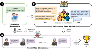
To give an extreme example of what a multi-step evaluation might look like, one recent paper found success in LLM evals by constructing multiple “personas” for different LLM agents, and having the agents debate in an actual courtroom structure:
Forcing different agents to advocate for different positions and examine each other’s arguments, all while having yet another agent act as a “judge” to emit a final decision, significantly increased the accuracy of evaluations.
In order for such a system to work, the handoffs between different agents must go smoothly. If an agent needs to pick between 5 possible actions, we need to be 100% sure that the model will only output one of those 5 valid actions. With structured generation, we can achieve that level of reliability.
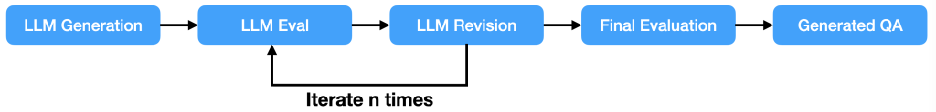
Let’s try a worked example, extending our hallucination metric from earlier. We’ll try the following improvement:
On first pass, the model will generate 3 candidate hallucinations, with reasoning for each.
For each candidate, the model will evaluate them individually and assess if they are a hallucination, with expanded reasoning.
If the model finds any candidate to be a hallucination, it will return 1.0 for the entire sample.
By giving the model the ability to generate longer chains of context, we give it space for more “intermediary computation,” and hopefully, a more accurate final output.
First, let’s define a series of prompts for this task:
generate_candidates_prompt = """ You are an expert judge tasked with evaluating the faithfulness of an AI-generated answer to a given context. Your goal is to determine if the provided output contains any hallucinations or unfaithful information when compared to the given context.
Here are the key elements you'll be working with:
1. <context>{context}</context> This is the factual information against which you must evaluate the output. All judgments of faithfulness must be based solely on this context.
2. <output>{output}</output> This is the AI-generated answer that you need to evaluate for faithfulness.
3. <input>{input}</input> This is the original question or prompt. It's provided for context only and should not be used in your faithfulness evaluation.
Evaluation Process: 1. Carefully read the CONTEXT and OUTPUT. 2. Analyze the OUTPUT for any discrepancies or additions when compared to the CONTEXT. 3. Consider the following aspects: - Does the OUTPUT introduce any new information not present in the CONTEXT? - Does the OUTPUT contradict any information given in the CONTEXT? - Does the OUTPUT contradict well-established facts or general knowledge? - Are there any partial hallucinations where some information is correct but other parts are not? - Is the subject of statements correct? Ensure that attributes, actions, or dates are correctly associated with the right entities. - Are there any subtle misattributions or conflations of information, even if dates or other details are correct? - Does the OUTPUT oversimplify or generalize information in a way that changes its meaning or accuracy?
4. Based on your analysis, create a list of 3 statements in the OUTPUT which are potentially hallucinations or unfaithful. For each potentially hallucinated or unfaithful statement from the OUTPUT, explain why you think it violates any of the aspects from step 3.
5. Return your list of statements and associated reasons in the following structured format:
Here is an example output structure (do not use these specific values, this is just to illustrate the format):
{{ "potential_hallucinations": [ {{ "output_statement": "The company was founded in 1995", "reasoning": "There is no mention of a founding date in the CONTEXT. The OUTPUT introduces new information not present in the CONTEXT. }}, {{ "output_statement": "The product costs $49.99.", "reasoning": "The CONTEXT lists the flagship product price at $39.99. The OUTPUT directly contradicts the price given in the CONTEXT." }}, {{ "output_statement": "The flagship product was their most expensive item.", "reasoning": "The CONTEXT lists mentions another product which is more expensive than the flagship product. The OUTPUT directly contradicts information given in the CONTEXT." }} ] }}
Now, please proceed with your analysis and evaluation of the provided INPUT, CONTEXT, and OUTPUT. """
evaluate_candidate_prompt = """ Please examine the following potential hallucination you detected in the OUTPUT:
{candidate}
You explained your reasons for flagging the statement like so:
{reason}
As a reminder, the CONTEXT you are evaluating the statement against is:
{context}
Based on the above, could you answer "yes" to any of the following questions? - Does the OUTPUT introduce any new information not present in the CONTEXT? - Does the OUTPUT contradict any information given in the CONTEXT? - Does the OUTPUT contradict well-established facts or general knowledge? - Are there any partial hallucinations where some information is correct but other parts are not? - Is the subject of statements correct? Ensure that attributes, actions, or dates are correctly associated with the right entities. - Are there any subtle misattributions or conflations of information, even if dates or other details are correct? - Does the OUTPUT oversimplify or generalize information in a way that changes its meaning or accuracy?
Please score the potentially hallucinated statement using the following scale:
- 1.0 if you answered "yes" to any of the previous questions, and you believe the statement is hallucinated or unfaithful to the CONTEXT. - 0.0 if you answered "no" to all of the previous questions, and after further reflection, you believe the statement is not hallucinated or unfaithful to the CONTEXT.
Before responding, please structure your response with the following format
{{ "score": float, "reason": string
}}
Here is an example output structure (do not use these specific values, this is just to illustrate the format):
{{ "score": 1.0, "reason": "The CONTEXT and OUTPUT list different prices for the same product. This leads me to answer 'yes' to the question, 'Does the OUTPUT contradict any information given in the CONTEXT?'" }}
Now, please proceed with your analysis and evaluation.
"""
And now, we can define some Pydantic models for our different model outputs:
# Generated by generate_candidates_prompt
class PotentialHallucination(pydantic.BaseModel):
    output_statement: str
    reasoning: str

class HallucinationCandidates(pydantic.BaseModel):
    potential_hallucinations: List[PotentialHallucination]

# Generated by evaluate_candidate_prompt
class HallucinationScore(pydantic.BaseModel):
    score: float
    reason: str
With all of this, we can put together two generators, one for generating candidate hallucinations, and one for scoring individual candidates:
import outlines
model_kwargs = { "device_map": "auto" }
model = outlines.models.transformers("Qwen/Qwen2.5-0.5B-Instruct", model_kwargs=model_kwargs)
Finally, we can construct an Opik metric. We’ll keep the code for this simple:
class HallucinationMultistep(base_metric.BaseMetric): """ A metric that evaluates whether an LLM's output contains hallucinations using a multi-step appraoch. """
# Initialize to zero, in case the model simply finds no candidates for hallucination score = HallucinationScore(score=0.0, reason="Found no candidates for hallucination")
for candidate in output.potential_hallucinations: followup_query = evaluate_candidate_prompt.format(candidate=candidate.output_statement, reason=candidate.reasoning, context=context) new_score = generator(followup_query) score = new_score if new_score.score > 0.0: # Early return if we find a hallucination return new_score
return score
All we do here is generate the first prompt, which should produce several hallucination candidates when fed to the candidate generator. Then, we pass each candidate (formatted with the candidate evaluation prompt) into the candidate evaluation generator.
If we run it using the same code as before, with slight modifications to use the new metric:
# Define the evaluation task def evaluation_task(x: Dict): # Use new metric metric = HallucinationMultistep() try: metric_score = metric.score( input=x["input"], context=x["context"], output=x["output"] ) hallucination_score = metric_score.score hallucination_reason = metric_score.reason except Exception as e: print(e) hallucination_score = None hallucination_reason = str(e)
# Define the scoring metric check_hallucinated_metric = Equals(name="Correct hallucination score")
res = evaluate( dataset=dataset, task=evaluation_task, scoring_metrics=[check_hallucinated_metric], )
Evaluation: 100%|██████████| 200/200 [19:02<00:00,  5.71s/it]
╭─  HaluEval-qa-samples Balanced (200 samples)   ─╮
│                                                 │
│ Total time:        00:19:03                     │
│ Number of samples: 200                          │
│                                                 │
│ Correct hallucination score: 0.5200 (avg)       │
│                                                 │
╰─────────────────────────────────────────────────╯
Uploading results to Opik ...
View the results in your Opik dashboard.
We see a great improvement. Remember that running this same model, with a very similar initial prompt, on this same dataset, resulted in a score of 0.46. By simply adding this additional candidate evaluation step, we immediately increased the score to 0.52. For such a small model, this is great!
Structured generation’s role in the future of LLM evaluations
Most foundation model providers, like OpenAI and Anthropic, offer some kind of structured output mode which will respond to your queries with a predefined schema. However, the world of LLM evaluations extends well beyond the closed ecosystems of these providers’ APIs.
For example:
So-called “white box” evaluations, which incorporate models’ internal states into the evaluation, are impossible with hosted models like GPT-4o.
Fine-tuning a model for your specific evaluation use-case requires you to use open source models.
If you need to run your evaluation pipeline locally, you obviously cannot use a hosted API.
And that’s without getting into comparisons of particular open source models against popular foundation models.
The future of LLM evaluations involves more complex evaluation suites, combining white box metrics, classic heuristic methods, and LLM judges into robust, multi-turn systems. Open source, or at the very least, locally-available LLMs are a major part of that future—and structured generation is a fundamental part of the infrastructure that is enabling that future.
We use cookies on our website to give you the most relevant experience by remembering your preferences and repeat visits. By clicking “Accept”, you consent to the use of ALL the cookies.
This website uses cookies to improve your experience while you navigate through the website. Out of these, the cookies that are categorized as necessary are stored on your browser as they are essential for the working of basic functionalities of the website. We also use third-party cookies that help us analyze and understand how you use this website. These cookies will be stored in your browser only with your consent. You also have the option to opt-out of these cookies. But opting out of some of these cookies may affect your browsing experience.
Necessary cookies are absolutely essential for the website to function properly. These cookies ensure basic functionalities and security features of the website, anonymously.
Cookie
Duration
Description
cookielawinfo-checkbox-analytics
11 months
This cookie is set by GDPR Cookie Consent plugin. The cookie is used to store the user consent for the cookies in the category "Analytics".
cookielawinfo-checkbox-functional
11 months
The cookie is set by GDPR cookie consent to record the user consent for the cookies in the category "Functional".
cookielawinfo-checkbox-necessary
11 months
This cookie is set by GDPR Cookie Consent plugin. The cookies is used to store the user consent for the cookies in the category "Necessary".
cookielawinfo-checkbox-others
11 months
This cookie is set by GDPR Cookie Consent plugin. The cookie is used to store the user consent for the cookies in the category "Other.
cookielawinfo-checkbox-performance
11 months
This cookie is set by GDPR Cookie Consent plugin. The cookie is used to store the user consent for the cookies in the category "Performance".
viewed_cookie_policy
11 months
The cookie is set by the GDPR Cookie Consent plugin and is used to store whether or not user has consented to the use of cookies. It does not store any personal data.
Functional cookies help to perform certain functionalities like sharing the content of the website on social media platforms, collect feedbacks, and other third-party features.
Performance cookies are used to understand and analyze the key performance indexes of the website which helps in delivering a better user experience for the visitors.
Analytical cookies are used to understand how visitors interact with the website. These cookies help provide information on metrics the number of visitors, bounce rate, traffic source, etc.
Advertisement cookies are used to provide visitors with relevant ads and marketing campaigns. These cookies track visitors across websites and collect information to provide customized ads.