Category: AI

  • Top 10 Data & AI Trends for 2025

    Top 10 Data & AI Trends for 2025

    Barr Moses

    Agentic AI, small data, and the search for value in the age of the unstructured data stack.

    Image credit: Monte Carlo

    According to industry experts, 2024 was destined to be a banner year for generative AI. Operational use cases were rising to the surface, technology was reducing barriers to entry, and general artificial intelligence was obviously right around the corner.

    So… did any of that happen?

    Well, sort of. Here at the end of 2024, some of those predictions have come out piping hot. The rest need a little more time in the oven (I’m looking at you general artificial intelligence).

    Here’s where leading futurist and investor Tomasz Tunguz thinks data and AI stands at the end of 2024 — plus a few predictions of my own.

    2025 data engineering trends incoming.

    1. We’re living in a world without reason (Tomasz)

    Just three years into our AI dystopia, we’re starting to see businesses create value in some of the areas we would expect — but not all of them. According to Tomasz, the current state of AI can be summed up in three categories.

    1. Prediction: AI copilots that can complete a sentence, correct code errors, etc.

    2. Search: tools that leverage a corpus of data to answer questions

    3. Reasoning: a multi-step workflow that can complete complex tasks

    While AI copilots and search have seen modest success (particularly the former) among enterprise orgs, reasoning models still appear to be lagging behind. And according to Tomasz, there’s an obvious reason for that.

    Model accuracy.

    As Tomasz explained, current models struggle to break down tasks into steps effectively unless they’ve seen a particular pattern many times before. And that’s just not the case for the bulk of the work these models could be asked to perform.

    “Today…if a large model were asked to produce an FP&A chart, it could do it. But if there’s some meaningful difference — for instance, we move from software billing to usage based billing — it will get lost.”

    So for now, it looks like its AI copilots and partially accurate search results for the win.

    2. Process > Tooling (Barr)

    A new tool is only as good as the process that supports it.

    As the “modern data stack” has continued to evolve over the years, data teams have sometimes found themselves in a state of perpetual tire-kicking. They would focus too heavily on the what of their platform without giving adequate attention to the (arguably more important) how.

    But as the enterprise landscape inches ever-closer toward production-ready AI — figuring out how to operationalize all this new tooling is becoming all the more urgent.

    Let’s consider the example of data quality for a moment. As the data feeding AI took center-stage in 2024, data quality took a step into the spotlight as well. Facing the real possibility of production-ready AI, enterprise data leaders don’t have time to sample from the data quality menu — a few dbt tests here, a couple point solutions there. They’re on the hook to deliver value now, and they need trusted solutions that they can onboard and deploy effectively today.

    As enterprise data leaders grapple with the near-term possibility of production-ready AI, they don’t have time to sample from the data quality menu — a few dbt tests here, a couple point solutions there. They’re already on the hook to deliver business value, and they need trusted solutions that they can onboard and deploy effectively today.

    The reality is, you could have the most sophisticated data quality platform on the market — the most advanced automations, the best copilots, the shiniest integrations — but if you can’t get your organization up and running quickly, all you’ve really got is a line item on your budget and a new tab on your desktop.

    Over the next 12 months, I expect data teams to lean into proven end-to-end solutions over patchwork toolkits in order to prioritize more critical challenges like data quality ownership, incident management, and long-term domain enablement.

    And the solution that delivers on those priorities is the solution that will win the day in AI.

    3. AI is driving ROI — but not revenue (Tomasz)

    Like any data product, GenAI’s value comes in one of two forms; reducing costs or generating revenue.

    On the revenue side, you might have something like AI SDRS, enrichment machines, or recommendations. According to Tomasz, these tools can generate a lot of sales pipeline… but it won’t be a healthy pipeline. So, if it’s not generating revenue, AI needs to be cutting costs — and in that regard, this budding technology has certainly found some footing.

    “Not many companies are closing business from it. It’s mostly cost reduction. Klarna cut two-thirds of their head count. Microsoft and ServiceNow have seen 50–75% increases in engineering productivity.”

    According to Tomasz, an AI use-case presents the opportunity for cost reduction if one of three criteria are met:

    • Repetitive jobs
    • Challenging labor market
    • Urgent hiring needs

    One example Tomasz cited of an organization that is driving new revenue effectively was EvenUp — a transactional legal company that automates demand letters. Organizations like EvenUp that support templated but highly specialized services could be uniquely positioned to see an outsized impact from AI in its current form.

    4. AI adoption is slower than expected — but leaders are biding their time (Tomasz)

    In contrast to the tsunami of “AI strategies” that were being embraced a year ago, leaders today seem to have taken a unanimous step backward from the technology.

    “There was a wave last year when people were trying all kinds of software just to see it. Their boards were asking about their AI strategy. But now there’s been a huge amount of churn in that early wave.”

    While some organizations simply haven’t seen value from their early experiments, others have struggled with the rapid evolution of its underlying technology. According to Tomasz, this is one of the biggest challenges for investing in AI companies. It’s not that the technology isn’t valuable in theory — it’s that organizations haven’t figured out how to leverage it effectively in practice.

    Tomasz believes that the next wave of adoption will be different from the first because leaders will be more informed about what they need — and where to find it.

    Like the dress rehearsal before the big show, teams know what they’re looking for, they’ve worked out some of the kinks with legal and procurement — particularly data loss and prevention — and they’re primed to act when the right opportunity presents itself.

    The big challenge of tomorrow? “How can I find and sell the value faster?”

    5. Small data is the future of AI (Tomasz)

    The open source versus managed debate is a tale as old as… well, something old. But when it comes to AI, that question gets a whole lot more complicated.

    At the enterprise level, it’s not simply a question of control or interoperability — though that can certainly play a part — it’s a question of operational cost.

    While Tomasz believes that the largest B2C companies will use off the shelf models, he expects B2B to trend toward their own proprietary and open-source models instead.

    “In B2B, you’ll see smaller models on the whole, and more open source on the whole. That’s because it’s much cheaper to run a small open source model.”

    But it’s not all dollars and cents. Small models also improve performance. Like Google, large models are designed to service a variety of use-cases. Users can ask a large model about effectively anything, so that model needs to be trained on a large enough corpus of data to deliver a relevant response. Water polo. Chinese history. French toast.

    Unfortunately, the more topics a model is trained on, the more likely it is to conflate multiple concepts — and the more erroneous the outputs will be over time.

    “You can take something like llama 2 with 8 billion parameters, fine tune it with 10,000 support tickets and it will perform much better,” says Tomasz.

    What’s more, ChatGPT and other managed solutions are frequently being challenged in courts over claims that their creators didn’t have legal rights to the data those models were trained on.

    And in many cases, that’s probably not wrong.

    This, in addition to cost and performance, will likely have an impact on long-term adoption of proprietary models — particulary in highly regulated industries — but the severity of that impact remains uncertain.

    Of course, proprietary models aren’t lying down either. Not if Sam Altman has anything to say about it. (And if Twitter has taught us anything, Sam Altman definitely has a lot to say.)

    Proprietary models are already aggressively cutting prices to drive demand. Models like ChatGPT have already cut prices by roughly 50% and are expecting to cut by another 50% in the next 6 months. That cost cutting could be a much needed boon for the B2C companies hoping to compete in the AI arms race.

    6. The lines are blurring for analysts and data engineers (Barr)

    When it comes to scaling pipeline production, there are generally two challenges that data teams will run into: analysts who don’t have enough technical experience and data engineers don’t have enough time.

    Sounds like a problem for AI.

    As we look to how data teams might evolve, there are two major developments that — I believe — could drive consolidation of engineering and analytical responsibilities in 2025:

    • Increased demand — as business leaders’ appetite for data and AI products grows, data teams will be on the hook to do more with less. In an effort to minimize bottlenecks, leaders will naturally empower previously specialized teams to absorb more responsibility for their pipelines — and their stakeholders.
    • Improvements in automation — new demand always drives new innovation. (In this case, that means AI-enabled pipelines.) As technologies naturally become more automated, engineers will be empowered to do more with less, while analysts will be empowered to do more on their own.

    The argument is simple — as demand increases, pipeline automation will naturally evolve to meet demand. As pipeline automation evolves to meet demand, the barrier to creating and managing those pipelines will decrease. The skill gap will decrease and the ability to add new value will increase.

    The move toward self-serve AI-enabled pipeline management means that the most painful part of everyone’s job gets automated away — and their ability to create and demonstrate new value expands in the process. Sounds like a nice future.

    7. Synthetic data matters — but it comes at a cost (Tomasz)

    You’ve probably seen the image of a snake eating its own tail. If you look closely, it bears a striking resemblance to contemporary AI.

    There are approximately 21–25 trillion tokens (words) on the internet right now. The AI models in production today have used all of them. In order for data to continue to advance, it requires an infinitely greater corpus of data to be trained on. The more data it has, the more context it has available for outputs — and the more accurate those outputs will be.

    So, what does an AI researcher do when they run out of training data?

    They make their own.

    As training data becomes more scarce, companies like OpenAI believe that synthetic data will be an important part of how they train their models in the future. And over the last 24 months, an entire industry has evolved to service that very vision — including companies like Tonic that generate synthetic structured data and Gretel that creates compliant data for regulated industries like finance and healthcare.

    But is synthetic data a long-term solution? Probably not.

    Synthetic data works by leveraging models to create artificial datasets that reflect what someone might find organically (in some alternate reality where more data actually exists), and then using that new data to train their own models. On a small scale, this actually makes a lot of sense. You know what they say about too much of a good thing…

    You can think of it like contextual malnutrition. Just like food, if a fresh organic data source is the most nutritious data for model training, then data that’s been distilled from existing datasets must be, by its nature, less nutrient rich than the data that came before.

    A little artificial flavoring is okay — but if that diet of synthetic training data continues into perpetuity without new grass-fed data being introduced, that model will eventually fail (or at the very least, have noticeably less attractive nail beds).

    It’s not really a matter of if, but when.

    According to Tomasz, we’re a long way off from model collapse at this point. But as AI research continues to push models to their functional limits, it’s not difficult to see a world where AI reaches its functional plateau — maybe sooner than later.

    8. The unstructured data stack will emerge (Barr)

    The idea of leveraging unstructured data in production isn’t new by any means — but in the age of AI, unstructured data has taken on a whole new role.

    According to a report by IDC only about half of an organization’s unstructured data is currently being analyzed.

    All that is about to change.

    When it comes to generative AI, enterprise success depends largely on the panoply of unstructured data that’s used to train, fine-tune, and augment it. As more organizations look to operationalize AI for enterprise use cases, enthusiasm for unstructured data — and the burgeoning “unstructured data stack” — will continue to grow as well.

    Some teams are even exploring how they can use additional LLMs to add structure to unstructured data to scale its usefulness in additional training and analytics use cases as well.

    Identifying what unstructured first-party data exists within your organization — and how you could potentially activate that data for your stakeholders — is a greenfield opportunity for data leaders looking to demonstrate the business value of their data platform (and hopefully secure some additional budget for priority initiatives along the way).

    If 2024 was about exploring the potential of unstructured data — 2025 will be all about realizing its value. The question is… what tools will rise to the surface?

    9. Agentic AI is great for conversation — but not deployment (Tomasz)

    If you’re swimming anywhere near the venture capital ponds these days, you’re likely to hear a couple terms tossed around pretty regularly: “copilot” which is a fancy term for an AI used to complete a single step (“correct my terrible code”), and “agents” which are a multi-step workflow that can gather information and use it to perform a task (“write a blog about my terrible code and publish it to my WordPress”).

    No doubt, we’ve seen a lot of success around AI copilots in 2024, (just ask Github, Snowflake, the Microsoft paperclip, etc), but what about AI agents?

    While “agentic AI” has had a fun time wreaking havoc on customer support teams, it looks like that’s all it’s destined to be in the near term. While these early AI agents are an important step forward, the accuracy of these workflows is still poor.

    For context, 75%-90% accuracy is state of the art for AI. Most AI is equivalent to a high school student. But if you have three steps of 75–90% accuracy, your ultimate accuracy is around 50%.

    We’ve trained elephants to paint with better accuracy than that.

    Far from being a revenue driver for organizations, most AI agents would be actively harmful if released into production at their current performance. According to Tomasz, we need to solve that problem first.

    It’s important to be able to talk about them, no one has had any success outside of a demo. Because regardless of how much people in the Valley might love to talk about AI agents, that talk doesn’t translate into performance.

    10. Pipelines are expanding — but quality coverage isn’t (Tomasz)

    “At a dinner with a bunch of heads of AI, I asked how many people were satisfied with the quality of the outputs, and no one raised their hands. There’s a real quality challenge in getting consistent outputs.”

    Pipelines are expanding and they need to be monitoring them. He was talking to an end to end AI solution. Everyone wants AI in the workflows, so the pipelines will increase dramatically. The quality of that data is absolutely essential. The pipelines are massively expanding and you need to be monitoring or you’ll be making the wrong decisions. And the data volumes will be increasingly tremendous.

    Each year, Monte Carlo surveys real data professionals about the state of their data quality. This year, we turned our gaze to the shadow of AI, and the message was clear.

    Data quality risks are evolving — but data quality management isn’t.

    “We’re seeing teams build out vector databases or embedding models at scale. SQLLite at scale. All of these 100 million small databases. They’re starting to be architected at the CDN layer to run all these small models. Iphones will have machine learning models. We’re going to see an explosion in the total number of pipelines but with much smaller data volumes.”

    The pattern of fine-tuning will create an explosion in the number of data pipelines within an organization. But the more pipelines expand, the more difficult data quality becomes.

    Data quality increases in direct proportion to the volume and complexity of your pipelines. The more pipelines you have (and the more complex they become), the more opportunities you’ll have for things to break — and the less likely you’ll be to find them in time.

    +++

    What do you think? Reach out to Barr at [email protected]. I’m all ears.


    Top 10 Data & AI Trends for 2025 was originally published in Towards Data Science on Medium, where people are continuing the conversation by highlighting and responding to this story.

    Originally appeared here:

    Top 10 Data & AI Trends for 2025

    Go Here to Read this Fast!

    Top 10 Data & AI Trends for 2025

  • AWS re:Invent 2024 Highlights: Top takeaways from Swami Sivasubramanian to help customers manage generative AI at scale

    AWS re:Invent 2024 Highlights: Top takeaways from Swami Sivasubramanian to help customers manage generative AI at scale

    Swami Sivasubramanian

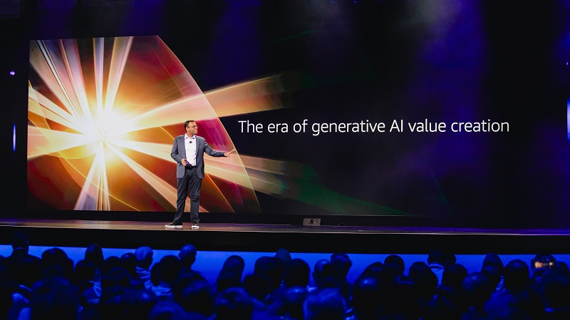
    We spoke with Dr. Swami Sivasubramanian, Vice President of Data and AI, shortly after AWS re:Invent 2024 to hear his impressions—and to get insights on how the latest AWS innovations help meet the real-world needs of customers as they build and scale transformative generative AI applications.

    Originally appeared here:
    AWS re:Invent 2024 Highlights: Top takeaways from Swami Sivasubramanian to help customers manage generative AI at scale

    Go Here to Read this Fast! AWS re:Invent 2024 Highlights: Top takeaways from Swami Sivasubramanian to help customers manage generative AI at scale

  • Multi-tenant RAG with Amazon Bedrock Knowledge Bases

    Multi-tenant RAG with Amazon Bedrock Knowledge Bases

    Emanuele Levi

    Organizations are continuously seeking ways to use their proprietary knowledge and domain expertise to gain a competitive edge. With the advent of foundation models (FMs) and their remarkable natural language processing capabilities, a new opportunity has emerged to unlock the value of their data assets. As organizations strive to deliver personalized experiences to customers using […]

    Originally appeared here:
    Multi-tenant RAG with Amazon Bedrock Knowledge Bases

    Go Here to Read this Fast! Multi-tenant RAG with Amazon Bedrock Knowledge Bases

  • Credit Card Fraud Detection with Different Sampling Techniques

    Mythili Krishnan

    How to deal with imbalanced data

    Photo by Bermix Studio on Unsplash

    Credit card fraud detection is a plague that all financial institutions are at risk with. In general fraud detection is very challenging because fraudsters are coming up with new and innovative ways of detecting fraud, so it is difficult to find a pattern that we can detect. For example, in the diagram all the icons look the same, but there one icon that is slightly different from the rest and we have pick that one. Can you spot it?

    Here it is:

    Image by Author

    With this background let me provide a plan for today and what you will learn in the context of our use case ‘Credit Card Fraud Detection’:

    1. What is data imbalance

    2. Possible causes of data Imbalance

    3. Why is class imbalance a problem in machine learning

    4. Quick Refresher on Random Forest Algorithm

    5. Different sampling methods to deal with data Imbalance

    6. Comparison of which method works well in our context with a practical Demonstration with Python

    7. Business insight on which model to choose and why?

    In most cases, because the number of fraudulent transactions is not a huge number, we have to work with a data that typically has a lot of non-frauds compared to Fraud cases. In technical terms such a dataset is called an ‘imbalanced data’. But, it is still essential to detect the fraud cases, because only 1 fraudulent transaction can cause millions of losses to banks/financial institutions. Now, let us delve deeper into what is data imbalance.

    We will be considering the credit card fraud dataset from https://www.kaggle.com/mlg-ulb/creditcardfraud (Open Data License).

    1. Data Imbalance

    Formally this means that the distribution of samples across different classes is unequal. In our case of binary classification problem, there are 2 classes

    a) Majority class—the non-fraudulent/genuine transactions

    b) Minority class—the fraudulent transactions

    In the dataset considered, the class distribution is as follows (Table 1):

    Table 1: Class Distribution (By Author)

    As we can observe, the dataset is highly imbalanced with only 0.17% of the observations being in the Fraudulent category.

    2. Possible causes of Data Imbalance

    There can be 2 main causes of data imbalance:

    a) Biased Sampling/Measurement errors: This is due to collection of samples only from one class or from a particular region or samples being mis-classified. This can be resolved by improving the sampling methods

    b) Use case/domain characteristic: A more pertinent problem as in our case might be due to the problem of prediction of a rare event, which automatically introduces skewness towards majority class because the occurrence of minor class is practice is not often.

    3. Why is class imbalance a problem in machine-learning?

    This is a problem because most of the algorithms in machine learning focus on learning from the occurrences that occur frequently i.e. the majority class. This is called the frequency bias. So in cases of imbalanced dataset, these algorithms might not work well. Typically few techniques that will work well are tree based algorithms or anomaly detection algorithms. Traditionally, in fraud detection problems business rule based methods are often used. Tree-based methods work well because a tree creates rule-based hierarchy that can separate both the classes. Decision trees tend to over-fit the data and to eliminate this possibility we will go with an ensemble method. For our use case, we will use the Random Forest Algorithm today.

    4. A quick Refresher on Random Forest Algorithm

    Random Forest works by building multiple decision tree predictors and the mode of the classes of these individual decision trees is the final selected class or output. It is like voting for the most popular class. For example: If 2 trees predict that Rule 1 indicates Fraud while another tree indicates that Rule 1 predicts Non-fraud, then according to Random forest algorithm the final prediction will be Fraud.

    Formal Definition: A random forest is a classifier consisting of a collection of tree-structured classifiers {h(x,Θk ), k=1, …} where the {Θk} are independent identically distributed random vectors and each tree casts a unit vote for the most popular class at input x . (Source)

    Each tree depends on a random vector that is independently sampled and all trees have a similar distribution. The generalization error converges as the number of trees increases. In its splitting criteria, Random forest searches for the best feature among a random subset of features and we can also compute variable importance and accordingly do feature selection. The trees can be grown using bagging technique where observations can be random selected (without replacement) from the training set. The other method can be random split selection where a random split is selected from K-best splits at each node.

    You can read more about it here

    5. Sampling methods to deal with Data Imbalance

    We will now illustrate 3 sampling methods that can take care of data imbalance.

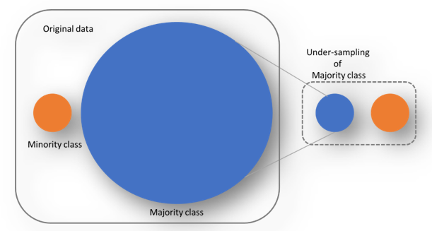
    a) Random Under-sampling: Random draws are taken from the non-fraud observations i.e the majority class to match it with the Fraud observations ie the minority class. This means, we are throwing away some information from the dataset which might not be ideal always.

    Fig 1: Random Under-sampling (Image By Author)

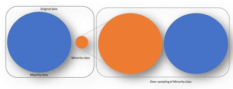
    b) Random Over-sampling: In this case, we do exact opposite of under-sampling i.e duplicate the minority class i.e Fraud observations at random to increase the number of the minority class till we get a balanced dataset. Possible limitation is we are creating a lot of duplicates with this method.

    Fig 2: Random Over-sampling (Image By Author)

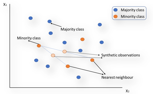
    c) SMOTE: (Synthetic Minority Over-sampling technique) is another method that uses synthetic data with KNN instead of using duplicate data. Each minority class example along with their k-nearest neighbours is considered. Then along the line segments that join any/all the minority class examples and k-nearest neighbours synthetic examples are created. This is illustrated in the Fig 3 below:

    Fig 3: SMOTE (Image By Author)

    With only over-sampling, the decision boundary becomes smaller while with SMOTE we can create larger decision regions thereby improving the chance of capturing the minority class better.

    One possible limitation is, if the minority class i.e fraudulent observations is spread throughout the data and not distinct then using nearest neighbours to create more fraud cases, introduces noise into the data and this can lead to mis-classification.

    6. Quick refresher on Accuracy, Recall, Precision

    Some of the metrics that is useful for judging the performance of a model are listed below. These metrics provide a view how well/how accurately the model is able to predict/classify the target variable/s:

    Fig 3: Classification Matrix (Image By Author)

    · TP (True positive)/TN (True negative) are the cases of correct predictions i.e predicting Fraud cases as Fraud (TP) and predicting non-fraud cases as non-fraud (TN)

    · FP (False positive) are those cases that are actually non-fraud but model predicts as Fraud

    · FN (False negative) are those cases that are actually fraud but model predicted as non-Fraud

    Precision = TP / (TP + FP): Precision measures how accurately model is able to capture fraud i.e out of the total predicted fraud cases, how many actually turned out to be fraud.

    Recall = TP/ (TP+FN): Recall measures out of all the actual fraud cases, how many the model could predict correctly as fraud. This is an important metric here.

    Accuracy = (TP +TN)/(TP+FP+FN+TN): Measures how many majority as well as minority classes could be correctly classified.

    F-score = 2*TP/ (2*TP + FP +FN) = 2* Precision *Recall/ (Precision *Recall) ; This is a balance between precision and recall. Note that precision and recall are inversely related, hence F-score is a good measure to achieve a balance between the two.

    7. Comparison of which method works well with a practical demonstration with Python

    First, we will train the random forest model with some default features. Please note optimizing the model with feature selection or cross validation has been kept out-of-scope here for sake of simplicity. Post that we train the model using under-sampling, oversampling and then SMOTE. The table below illustrates the confusion matrix along with the precision, recall and accuracy metrics for each method.

    Table 2: Model results comparison (By Author)

    a) No sampling result interpretation: Without any sampling we are able to capture 76 fraudulent transactions. Though the overall accuracy is 97%, the recall is 75%. This means that there are quite a few fraudulent transactions that our model is not able to capture.

    Below is the code that can be used :

    # Training the model
    from sklearn.ensemble import RandomForestClassifier
    classifier = RandomForestClassifier(n_estimators=10,criterion='entropy', random_state=0)
    classifier.fit(x_train,y_train)

    # Predict Y on the test set
    y_pred = classifier.predict(x_test)

    # Obtain the results from the classification report and confusion matrix
    from sklearn.metrics import classification_report, confusion_matrix

    print('Classifcation report:n', classification_report(y_test, y_pred))
    conf_mat = confusion_matrix(y_true=y_test, y_pred=y_pred)
    print('Confusion matrix:n', conf_mat)

    b) Under-sampling result interpretation: With under-sampling , though the model is able to capture 90 fraud cases with significant improvement in recall, the accuracy and precision falls drastically. This is because the false positives have increased phenomenally and the model is penalizing a lot of genuine transactions.

    Under-sampling code snippet:

    # This is the pipeline module we need from imblearn
    from imblearn.under_sampling import RandomUnderSampler
    from imblearn.pipeline import Pipeline

    # Define which resampling method and which ML model to use in the pipeline
    resampling = RandomUnderSampler()
    model = RandomForestClassifier(n_estimators=10,criterion='entropy', random_state=0)

    # Define the pipeline,and combine sampling method with the RF model
    pipeline = Pipeline([('RandomUnderSampler', resampling), ('RF', model)])

    pipeline.fit(x_train, y_train)
    predicted = pipeline.predict(x_test)

    # Obtain the results from the classification report and confusion matrix
    print('Classifcation report:n', classification_report(y_test, predicted))
    conf_mat = confusion_matrix(y_true=y_test, y_pred=predicted)
    print('Confusion matrix:n', conf_mat)

    c) Over-sampling result interpretation: Over-sampling method has the highest precision and accuracy and the recall is also good at 81%. We are able to capture 6 more fraud cases and the false positives is pretty low as well. Overall, from the perspective of all the parameters, this model is a good model.

    Oversampling code snippet:

    # This is the pipeline module we need from imblearn
    from imblearn.over_sampling import RandomOverSampler

    # Define which resampling method and which ML model to use in the pipeline
    resampling = RandomOverSampler()
    model = RandomForestClassifier(n_estimators=10,criterion='entropy', random_state=0)

    # Define the pipeline,and combine sampling method with the RF model
    pipeline = Pipeline([('RandomOverSampler', resampling), ('RF', model)])

    pipeline.fit(x_train, y_train)
    predicted = pipeline.predict(x_test)

    # Obtain the results from the classification report and confusion matrix
    print('Classifcation report:n', classification_report(y_test, predicted))
    conf_mat = confusion_matrix(y_true=y_test, y_pred=predicted)
    print('Confusion matrix:n', conf_mat)

    d) SMOTE: Smote further improves the over-sampling method with 3 more frauds caught in the net and though false positives increase a bit the recall is pretty healthy at 84%.

    SMOTE code snippet:

    # This is the pipeline module we need from imblearn

    from imblearn.over_sampling import SMOTE


    # Define which resampling method and which ML model to use in the pipeline
    resampling = SMOTE(sampling_strategy='auto',random_state=0)
    model = RandomForestClassifier(n_estimators=10,criterion='entropy', random_state=0)

    # Define the pipeline, tell it to combine SMOTE with the RF model
    pipeline = Pipeline([('SMOTE', resampling), ('RF', model)])

    pipeline.fit(x_train, y_train)
    predicted = pipeline.predict(x_test)

    # Obtain the results from the classification report and confusion matrix
    print('Classifcation report:n', classification_report(y_test, predicted))
    conf_mat = confusion_matrix(y_true=y_test, y_pred=predicted)
    print('Confusion matrix:n', conf_mat)

    Summary:

    In our use case of fraud detection, the one metric that is most important is recall. This is because the banks/financial institutions are more concerned about catching most of the fraud cases because fraud is expensive and they might lose a lot of money over this. Hence, even if there are few false positives i.e flagging of genuine customers as fraud it might not be too cumbersome because this only means blocking some transactions. However, blocking too many genuine transactions is also not a feasible solution, hence depending on the risk appetite of the financial institution we can go with either simple over-sampling method or SMOTE. We can also tune the parameters of the model, to further enhance the model results using grid search.

    For details on the code refer to this link on Github.

    References:

    [1] Mythili Krishnan, Madhan K. Srinivasan, Credit Card Fraud Detection: An Exploration of Different Sampling Methods to Solve the Class Imbalance Problem (2022), ResearchGate

    [1] Bartosz Krawczyk, Learning from imbalanced data: open challenges and future directions (2016), Springer

    [2] Nitesh V. Chawla, Kevin W. Bowyer , Lawrence O. Hall and W. Philip Kegelmeyer , SMOTE: Synthetic Minority Over-sampling Technique (2002), Journal of Artificial Intelligence research

    [3] Leo Breiman, Random Forests (2001), stat.berkeley.edu

    [4] Jeremy Jordan, Learning from imbalanced data (2018)

    [5] https://trenton3983.github.io/files/projects/2019-07-19_fraud_detection_python/2019-07-19_fraud_detection_python.html


    Credit Card Fraud Detection with Different Sampling Techniques was originally published in Towards Data Science on Medium, where people are continuing the conversation by highlighting and responding to this story.

    Originally appeared here:
    Credit Card Fraud Detection with Different Sampling Techniques

    Go Here to Read this Fast! Credit Card Fraud Detection with Different Sampling Techniques

  • API Design of X (Twitter) Home Timeline

    API Design of X (Twitter) Home Timeline

    Oleksii Trekhleb

    How X (Twitter) Designed Its Home Timeline API: Lessons to Learn

    A closer look at X’s API: fetching data, linking entities, and solving under-fetching.

    When designing a system’s API, software engineers often evaluate various approaches, such as REST vs RPC vs GraphQL, or hybrid models, to determine the best fit for a specific task or project. These approaches define how data flows between the backend and frontend, as well as the structure of the response data:

    • Should all data be packed into a single “batch” and returned in one response?
    • Can the “batch” be configured to include only the required fields for a specific client (e.g., browser vs. mobile) to avoid over-fetching?
    • What happens if the client under-fetches data and requires additional backend calls to retrieve missing entities?
    • How should parent-child relationships be handled? Should child entities be embedded within their parent, or should normalization be applied, where parent entities only reference child entity IDs to improve reusability and reduce response size?

    In this article, we explore how the X (formerly Twitter) home timeline API (x.com/home) addresses these challenges, including:

    • Fetching the list of tweets
    • Returning hierarchical or linked data (e.g., tweets, users, media)
    • Sorting and paginating results
    • Retrieving tweet details
    • Liking a tweet

    Our focus will be on the API design and functionality, treating the backend as a black box since its implementation is inaccessible.

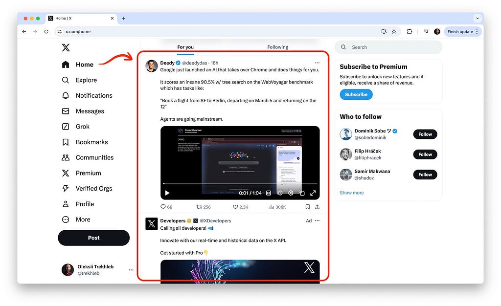
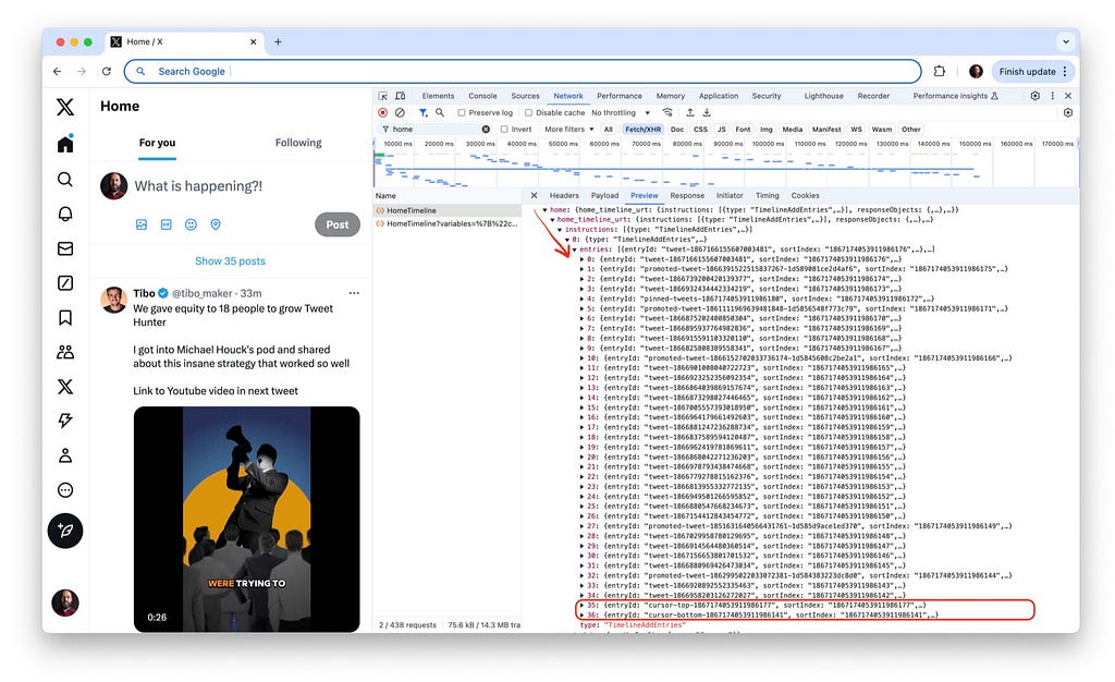
    Example of X home timeline

    Showing the exact requests and responses here might be cumbersome and hard to follow since the deeply nested and repetitive objects are hard to read. To make it easier to see the request/response payload structure, I’ve made my attempt to “type out” the home timeline API in TypeScript. So when it comes to the request/response examples I’ll use the request and response types instead of actual JSON objects. Also, remember that the types are simplified and many properties are omitted for brevity.

    You may find all types in types/x.ts file or at the bottom of this article in the “Appendix: All types at one place” section.

    All images, unless othewise noted, are by the author.

    Fetching the list of tweets

    The endpoint and request/response structure

    Fetching the list of tweets for the home timeline starts with the POST request to the following endpoint:

    POST https://x.com/i/api/graphql/{query-id}/HomeTimeline

    Here is a simplified request body type:

    type TimelineRequest = {
    queryId: string; // 's6ERr1UxkxxBx4YundNsXw'
    variables: {
    count: number; // 20
    cursor?: string; // 'DAAACgGBGedb3Vx__9sKAAIZ5g4QENc99AcAAwAAIAIAAA'
    seenTweetIds: string[]; // ['1867041249938530657', '1867041249938530659']
    };
    features: Features;
    };

    type Features = {
    articles_preview_enabled: boolean;
    view_counts_everywhere_api_enabled: boolean;
    // ...
    }

    Here is a simplified response body type (we’ll dive deeper into the response sub-types below):

    type TimelineResponse = {
    data: {
    home: {
    home_timeline_urt: {
    instructions: (TimelineAddEntries | TimelineTerminateTimeline)[];
    responseObjects: {
    feedbackActions: TimelineAction[];
    };
    };
    };
    };
    };

    type TimelineAddEntries = {
    type: 'TimelineAddEntries';
    entries: (TimelineItem | TimelineCursor | TimelineModule)[];
    };

    type TimelineItem = {
    entryId: string; // 'tweet-1867041249938530657'
    sortIndex: string; // '1866561576636152411'
    content: {
    __typename: 'TimelineTimelineItem';
    itemContent: TimelineTweet;
    feedbackInfo: {
    feedbackKeys: ActionKey[]; // ['-1378668161']
    };
    };
    };

    type TimelineTweet = {
    __typename: 'TimelineTweet';
    tweet_results: {
    result: Tweet;
    };
    };

    type TimelineCursor = {
    entryId: string; // 'cursor-top-1867041249938530657'
    sortIndex: string; // '1866961576813152212'
    content: {
    __typename: 'TimelineTimelineCursor';
    value: string; // 'DACBCgABGedb4VyaJwuKbIIZ40cX3dYwGgaAAwAEAEEAA'
    cursorType: 'Top' | 'Bottom';
    };
    };

    type ActionKey = string;

    It is interesting to note here, that “getting” the data is done via “POSTing”, which is not common for the REST-like API but it is common for a GraphQL-like API. Also, the graphql part of the URL indicates that X is using the GraphQL flavor for their API.

    I’m using the word “flavor” here because the request body itself doesn’t look like a pure GraphQL query, where we may describe the required response structure, listing all the properties we want to fetch:

    # An example of a pure GraphQL request structure that is *not* being used in the X API.
    {
    tweets {
    id
    description
    created_at
    medias {
    kind
    url
    # ...
    }
    author {
    id
    name
    # ...
    }
    # ...
    }
    }

    The assumption here is that the home timeline API is not a pure GraphQL API, but is a mix of several approaches. Passing the parameters in a POST request like this seems closer to the “functional” RPC call. But at the same time, it seems like the GraphQL features might be used somewhere on the backend behind the HomeTimeline endpoint handler/controller. A mix like this might also be caused by a legacy code or some sort of ongoing migration. But again, these are just my speculations.

    You may also notice that the same TimelineRequest.queryId is used in the API URL as well as in the API request body. This queryId is most probably generated on the backend, then it gets embedded in the main.js bundle, and then it is used when fetching the data from the backend. It is hard for me to understand how this queryId is used exactly since X’s backend is a black box in our case. But, again, the speculation here might be that, it might be needed for some sort of performance optimization (re-using some pre-computed query results?), caching (Apollo related?), debugging (join logs by queryId?), or tracking/tracing purposes.

    It is also interesting to note, that the TimelineResponse contains not a list of tweets, but rather a list of instructions, like “add a tweet to the timeline” (see the TimelineAddEntries type), or “terminate the timeline” (see the TimelineTerminateTimeline type).

    The TimelineAddEntries instruction itself may also contain different types of entities:

    • Tweets — see the TimelineItem type
    • Cursors — see the TimelineCursor type
    • Conversations/comments/threads — see the TimelineModule type
    type TimelineResponse = {
    data: {
    home: {
    home_timeline_urt: {
    instructions: (TimelineAddEntries | TimelineTerminateTimeline)[]; // <-- Here
    // ...
    };
    };
    };
    };

    type TimelineAddEntries = {
    type: 'TimelineAddEntries';
    entries: (TimelineItem | TimelineCursor | TimelineModule)[]; // <-- Here
    };

    This is interesting from the extendability point of view since it allows a wider variety of what can be rendered in the home timeline without tweaking the API too much.

    Pagination

    The TimelineRequest.variables.count property sets how many tweets we want to fetch at once (per page). The default is 20. However, more than 20 tweets can be returned in the TimelineAddEntries.entries array. For example, the array might contain 37 entries for the first page load, because it includes tweets (29), pinned tweets (1), promoted tweets (5), and pagination cursors (2). I’m not sure why there are 29 regular tweets with the requested count of 20 though.

    The TimelineRequest.variables.cursor is responsible for the cursor-based pagination.

    “Cursor pagination is most often used for real-time data due to the frequency new records are added and because when reading data you often see the latest results first. It eliminates the possibility of skipping items and displaying the same item more than once. In cursor-based pagination, a constant pointer (or cursor) is used to keep track of where in the data set the next items should be fetched from.” See the Offset pagination vs Cursor pagination thread for the context.

    When fetching the list of tweets for the first time the TimelineRequest.variables.cursor is empty, since we want to fetch the top tweets from the default (most probably pre-computed) list of personalized tweets.

    However, in the response, along with the tweet data, the backend also returns the cursor entries. Here is the response type hierarchy: TimelineResponse → TimelineAddEntries → TimelineCursor:

    type TimelineResponse = {
    data: {
    homet: {
    home_timeline_urt: {
    instructions: (TimelineAddEntries | TimelineTerminateTimeline)[]; // <-- Here
    // ...
    };
    };
    };
    };

    type TimelineAddEntries = {
    type: 'TimelineAddEntries';
    entries: (TimelineItem | TimelineCursor | TimelineModule)[]; // <-- Here (tweets + cursors)
    };

    type TimelineCursor = {
    entryId: string;
    sortIndex: string;
    content: {
    __typename: 'TimelineTimelineCursor';
    value: string; // 'DACBCgABGedb4VyaJwuKbIIZ40cX3dYwGgaAAwAEAEEAA' <-- Here
    cursorType: 'Top' | 'Bottom';
    };
    };

    Every page contains the list of tweets along with “top” and “bottom” cursors:

    Examples of how cursors are passed along with tweets

    After the page data is loaded, we can go from the current page in both directions and fetch either the “previous/older” tweets using the “bottom” cursor or the “next/newer” tweets using the “top” cursor. My assumption is that fetching the “next” tweets using the “top” cursor happens in two cases: when the new tweets were added while the user is still reading the current page, or when the user starts scrolling the feed upwards (and there are no cached entries or if the previous entries were deleted for the performance reasons).

    The X’s cursor itself might look like this: DAABCgABGemI6Mk__9sKAAIZ6MSYG9fQGwgAAwAAAAIAAA. In some API designs, the cursor may be a Base64 encoded string that contains the id of the last entry in the list, or the timestamp of the last seen entry. For example: eyJpZCI6ICIxMjM0NTY3ODkwIn0= –> {“id”: “1234567890”}, and then, this data is used to query the database accordingly. In the case of X API, it looks like the cursor is being Base64 decoded into some custom binary sequence that might require some further decoding to get any meaning out of it (i.e. via the Protobuf message definitions). Since we don’t know if it is a .proto encoding and also we don’t know the .proto message definition we may just assume that the backend knows how to query the next batch of tweets based on the cursor string.

    The TimelineResponse.variables.seenTweetIds parameter is used to inform the server about which tweets from the currently active page of the infinite scrolling the client has already seen. This most probably helps ensure that the server does not include duplicate tweets in subsequent pages of results.

    Linked/hierarchical entities

    One of the challenges to be solved in the APIs like home timeline (or Home Feed) is to figure out how to return the linked or hierarchical entities (i.e. tweet → user, tweet → media, media → author, etc):

    • Should we only return the list of tweets first and then fetch the dependent entities (like user details) in a bunch of separate queries on-demand?
    • Or should we return all the data at once, increasing the time and the size of the first load, but saving the time for all subsequent calls?
    • Do we need to normalize the data in this case to reduce the payload size (i.e. when the same user is an author of many tweets and we want to avoid repeating the user data over and over again in each tweet entity)?
    • Or should it be a combination of the approaches above?

    Let’s see how X handles it.

    Earlier in the TimelineTweet type the Tweet sub-type was used. Let’s see how it looks:

    export type TimelineResponse = {
    data: {
    home: {
    home_timeline_urt: {
    instructions: (TimelineAddEntries | TimelineTerminateTimeline)[]; // <-- Here
    // ...
    };
    };
    };
    };

    type TimelineAddEntries = {
    type: 'TimelineAddEntries';
    entries: (TimelineItem | TimelineCursor | TimelineModule)[]; // <-- Here
    };

    type TimelineItem = {
    entryId: string;
    sortIndex: string;
    content: {
    __typename: 'TimelineTimelineItem';
    itemContent: TimelineTweet; // <-- Here
    // ...
    };
    };

    type TimelineTweet = {
    __typename: 'TimelineTweet';
    tweet_results: {
    result: Tweet; // <-- Here
    };
    };

    // A Tweet entity
    type Tweet = {
    __typename: 'Tweet';
    core: {
    user_results: {
    result: User; // <-- Here (a dependent User entity)
    };
    };
    legacy: {
    full_text: string;
    // ...
    entities: { // <-- Here (a dependent Media entities)
    media: Media[];
    hashtags: Hashtag[];
    urls: Url[];
    user_mentions: UserMention[];
    };
    };
    };

    // A User entity
    type User = {
    __typename: 'User';
    id: string; // 'VXNlcjoxNDUxM4ADSG44MTA4NDc4OTc2'
    // ...
    legacy: {
    location: string; // 'San Francisco'
    name: string; // 'John Doe'
    // ...
    };
    };

    // A Media entity
    type Media = {
    // ...
    source_user_id_str: string; // '1867041249938530657' <-- Here (the dependant user is being mentioned by its ID)
    url: string; // 'https://t.co/X78dBgtrsNU'
    features: {
    large: { faces: FaceGeometry[] };
    medium: { faces: FaceGeometry[] };
    small: { faces: FaceGeometry[] };
    orig: { faces: FaceGeometry[] };
    };
    sizes: {
    large: MediaSize;
    medium: MediaSize;
    small: MediaSize;
    thumb: MediaSize;
    };
    video_info: VideoInfo[];
    };

    What’s interesting here is that most of the dependent data like tweet → media and tweet → author is embedded into the response on the first call (no subsequent queries).

    Also, the User and Media connections with Tweet entities are not normalized (if two tweets have the same author, their data will be repeated in each tweet object). But it seems like it should be ok, since in the scope of the home timeline for a specific user the tweets will be authored by many authors and repetitions are possible but sparse.

    My assumption was that the UserTweets API (that we don’t cover here), which is responsible for fetching the tweets of one particular user will handle it differently, but, apparently, it is not the case. The UserTweets returns the list of tweets of the same user and embeds the same user data over and over again for each tweet. It’s interesting. Maybe the simplicity of the approach beats some data size overhead (maybe user data is considered pretty small in size). I’m not sure.

    Another observation about the entities’ relationship is that the Media entity also has a link to the User (the author). But it does it not via direct entity embedding as the Tweet entity does, but rather it links via the Media.source_user_id_str property.

    The “comments” (which are also the “tweets” by their nature) for each “tweet” in the home timeline are not fetched at all. To see the tweet thread the user must click on the tweet to see its detailed view. The tweet thread will be fetched by calling the TweetDetail endpoint (more about it in the “Tweet detail page” section below).

    Another entity that each Tweet has is FeedbackActions (i.e. “Recommend less often” or “See fewer”). The way the FeedbackActions are stored in the response object is different from the way the User and Media objects are stored. While the User and Media entities are part of the Tweet, the FeedbackActions are stored separately in TimelineItem.content.feedbackInfo.feedbackKeys array and are linked via the ActionKey. That was a slight surprise for me since it doesn’t seem to be the case that any action is re-usable. It looks like one action is used for one particular tweet only. So it seems like the FeedbackActions could be embedded into each tweet in the same way as Media entities. But I might be missing some hidden complexity here (like the fact that each action can have children actions).

    More details about the actions are in the “Tweet actions” section below.

    Sorting

    The sorting order of the timeline entries is defined by the backend via the sortIndex properties:

    type TimelineCursor = {
    entryId: string;
    sortIndex: string; // '1866961576813152212' <-- Here
    content: {
    __typename: 'TimelineTimelineCursor';
    value: string;
    cursorType: 'Top' | 'Bottom';
    };
    };

    type TimelineItem = {
    entryId: string;
    sortIndex: string; // '1866561576636152411' <-- Here
    content: {
    __typename: 'TimelineTimelineItem';
    itemContent: TimelineTweet;
    feedbackInfo: {
    feedbackKeys: ActionKey[];
    };
    };
    };

    type TimelineModule = {
    entryId: string;
    sortIndex: string; // '73343543020642838441' <-- Here
    content: {
    __typename: 'TimelineTimelineModule';
    items: {
    entryId: string,
    item: TimelineTweet,
    }[],
    displayType: 'VerticalConversation',
    };
    };

    The sortIndex itself might look something like this ‘1867231621095096312’. It likely corresponds directly to or is derived from a Snowflake ID.

    Actually most of the IDs you see in the response (tweet IDs) follow the “Snowflake ID” convention and look like ‘1867231621095096312’.

    If this is used to sort entities like tweets, the system leverages the inherent chronological sorting of Snowflake IDs. Tweets or objects with a higher sortIndex value (a more recent timestamp) appear higher in the feed, while those with lower values (an older timestamp) appear lower in the feed.

    Here’s the step-by-step decoding of the Snowflake ID (in our case the sortIndex) 1867231621095096312:

    • Extract the Timestamp:
    • The timestamp is derived by right-shifting the Snowflake ID by 22 bits (to remove the lower 22 bits for data center, worker ID, and sequence): 1867231621095096312 → 445182709954
    • Add Twitter’s Epoch:
    • Adding Twitter’s custom epoch (1288834974657) to this timestamp gives the UNIX timestamp in milliseconds: 445182709954 + 1288834974657 → 1734017684611ms
    • Convert to a human-readable date:
    • Converting the UNIX timestamp to a UTC datetime gives: 1734017684611ms → 2024-12-12 15:34:44.611 (UTC)

    So we can assume here that the tweets in the home timeline are sorted chronologically.

    Tweet actions

    Each tweet has an “Actions” menu.

    Example of tweet actions

    The actions for each tweet are coming from the backend in a TimelineItem.content.feedbackInfo.feedbackKeys array and are linked with the tweets via the ActionKey:

    type TimelineResponse = {
    data: {
    home: {
    home_timeline_urt: {
    instructions: (TimelineAddEntries | TimelineTerminateTimeline)[];
    responseObjects: {
    feedbackActions: TimelineAction[]; // <-- Here
    };
    };
    };
    };
    };

    type TimelineItem = {
    entryId: string;
    sortIndex: string;
    content: {
    __typename: 'TimelineTimelineItem';
    itemContent: TimelineTweet;
    feedbackInfo: {
    feedbackKeys: ActionKey[]; // ['-1378668161'] <-- Here
    };
    };
    };

    type TimelineAction = {
    key: ActionKey; // '-609233128'
    value: {
    feedbackType: 'NotRelevant' | 'DontLike' | 'SeeFewer'; // ...
    prompt: string; // 'This post isn’t relevant' | 'Not interested in this post' | ...
    confirmation: string; // 'Thanks. You’ll see fewer posts like this.'
    childKeys: ActionKey[]; // ['1192182653', '-1427553257'], i.e. NotInterested -> SeeFewer
    feedbackUrl: string; // '/2/timeline/feedback.json?feedback_type=NotRelevant&action_metadata=SRwW6oXZadPHiOczBBaAwPanEwE%3D'
    hasUndoAction: boolean;
    icon: string; // 'Frown'
    };
    };

    It is interesting here that this flat array of actions is actually a tree (or a graph? I didn’t check), since each action may have child actions (see the TimelineAction.value.childKeys array). This makes sense, for example, when after the user clicks on the “Don’t Like” action, the follow-up might be to show the “This post isn’t relevant” action, as a way of explaining why the user doesn’t like the tweet.

    Tweet detail page

    Once the user would like to see the tweet detail page (i.e. to see the thread of comments/tweets), the user clicks on the tweet and the GET request to the following endpoint is performed:

    GET https://x.com/i/api/graphql/{query-id}/TweetDetail?variables={"focalTweetId":"1867231621095096312","referrer":"home","controller_data":"DACABBSQ","rankingMode":"Relevance","includePromotedContent":true,"withCommunity":true}&features={"articles_preview_enabled":true}

    I was curious here why the list of tweets is being fetched via the POST call, but each tweet detail is fetched via the GET call. Seems inconsistent. Especially keeping in mind that similar query parameters like query-id, features, and others this time are passed in the URL and not in the request body. The response format is also similar and is re-using the types from the list call. I’m not sure why is that. But again, I’m sure I might be might be missing some background complexity here.

    Here are the simplified response body types:

    type TweetDetailResponse = {
    data: {
    threaded_conversation_with_injections_v2: {
    instructions: (TimelineAddEntries | TimelineTerminateTimeline)[],
    },
    },
    }

    type TimelineAddEntries = {
    type: 'TimelineAddEntries';
    entries: (TimelineItem | TimelineCursor | TimelineModule)[];
    };

    type TimelineTerminateTimeline = {
    type: 'TimelineTerminateTimeline',
    direction: 'Top',
    }

    type TimelineModule = {
    entryId: string; // 'conversationthread-58668734545929871193'
    sortIndex: string; // '1867231621095096312'
    content: {
    __typename: 'TimelineTimelineModule';
    items: {
    entryId: string, // 'conversationthread-1866876425669871193-tweet-1866876038930951193'
    item: TimelineTweet,
    }[], // Comments to the tweets are also tweets
    displayType: 'VerticalConversation',
    };
    };

    The response is pretty similar (in its types) to the list response, so we won’t for too long here.

    One interesting nuance is that the “comments” (or conversations) of each tweet are actually other tweets (see the TimelineModule type). So the tweet thread looks very similar to the home timeline feed by showing the list of TimelineTweet entries. This looks elegant. A good example of a universal and re-usable approach to the API design.

    Liking the tweet

    When a user likes the tweet, the POST request to the following endpoint is being performed:

    POST https://x.com/i/api/graphql/{query-id}/FavoriteTweet

    Here is the request body types:

    type FavoriteTweetRequest = {
    variables: {
    tweet_id: string; // '1867041249938530657'
    };
    queryId: string; // 'lI07N61twFgted2EgXILM7A'
    };

    Here is the response body types:

    type FavoriteTweetResponse = {
    data: {
    favorite_tweet: 'Done',
    }
    }

    Looks straightforward and also resembles the RPC-like approach to the API design.

    Conclusion

    We have touched on some basic parts of the home timeline API design by looking at X’s API example. I made some assumptions along the way to the best of my knowledge. I believe some things I might have interpreted incorrectly and I might have missed some complex nuances. But even with that in mind, I hope you got some useful insights from this high-level overview, something that you could apply in your next API Design session.

    Initially, I had a plan to go through similar top-tech websites to get some insights from Facebook, Reddit, YouTube, and others and to collect battle-tested best practices and solutions. I’m not sure if I’ll find the time to do that. Will see. But it could be an interesting exercise.

    Appendix: All types in one place

    For the reference, I’m adding all types in one go here. You may also find all types in types/x.ts file.

    /**
    * This file contains the simplified types for X's (Twitter's) home timeline API.
    *
    * These types are created for exploratory purposes, to see the current implementation
    * of the X's API, to see how they fetch Home Feed, how they do a pagination and sorting,
    * and how they pass the hierarchical entities (posts, media, user info, etc).
    *
    * Many properties and types are omitted for simplicity.
    */

    // POST https://x.com/i/api/graphql/{query-id}/HomeTimeline
    export type TimelineRequest = {
    queryId: string; // 's6ERr1UxkxxBx4YundNsXw'
    variables: {
    count: number; // 20
    cursor?: string; // 'DAAACgGBGedb3Vx__9sKAAIZ5g4QENc99AcAAwAAIAIAAA'
    seenTweetIds: string[]; // ['1867041249938530657', '1867041249938530658']
    };
    features: Features;
    };

    // POST https://x.com/i/api/graphql/{query-id}/HomeTimeline
    export type TimelineResponse = {
    data: {
    home: {
    home_timeline_urt: {
    instructions: (TimelineAddEntries | TimelineTerminateTimeline)[];
    responseObjects: {
    feedbackActions: TimelineAction[];
    };
    };
    };
    };
    };

    // POST https://x.com/i/api/graphql/{query-id}/FavoriteTweet
    export type FavoriteTweetRequest = {
    variables: {
    tweet_id: string; // '1867041249938530657'
    };
    queryId: string; // 'lI07N6OtwFgted2EgXILM7A'
    };

    // POST https://x.com/i/api/graphql/{query-id}/FavoriteTweet
    export type FavoriteTweetResponse = {
    data: {
    favorite_tweet: 'Done',
    }
    }

    // GET https://x.com/i/api/graphql/{query-id}/TweetDetail?variables={"focalTweetId":"1867041249938530657","referrer":"home","controller_data":"DACABBSQ","rankingMode":"Relevance","includePromotedContent":true,"withCommunity":true}&features={"articles_preview_enabled":true}
    export type TweetDetailResponse = {
    data: {
    threaded_conversation_with_injections_v2: {
    instructions: (TimelineAddEntries | TimelineTerminateTimeline)[],
    },
    },
    }

    type Features = {
    articles_preview_enabled: boolean;
    view_counts_everywhere_api_enabled: boolean;
    // ...
    }

    type TimelineAction = {
    key: ActionKey; // '-609233128'
    value: {
    feedbackType: 'NotRelevant' | 'DontLike' | 'SeeFewer'; // ...
    prompt: string; // 'This post isn’t relevant' | 'Not interested in this post' | ...
    confirmation: string; // 'Thanks. You’ll see fewer posts like this.'
    childKeys: ActionKey[]; // ['1192182653', '-1427553257'], i.e. NotInterested -> SeeFewer
    feedbackUrl: string; // '/2/timeline/feedback.json?feedback_type=NotRelevant&action_metadata=SRwW6oXZadPHiOczBBaAwPanEwE%3D'
    hasUndoAction: boolean;
    icon: string; // 'Frown'
    };
    };

    type TimelineAddEntries = {
    type: 'TimelineAddEntries';
    entries: (TimelineItem | TimelineCursor | TimelineModule)[];
    };

    type TimelineTerminateTimeline = {
    type: 'TimelineTerminateTimeline',
    direction: 'Top',
    }

    type TimelineCursor = {
    entryId: string; // 'cursor-top-1867041249938530657'
    sortIndex: string; // '1867231621095096312'
    content: {
    __typename: 'TimelineTimelineCursor';
    value: string; // 'DACBCgABGedb4VyaJwuKbIIZ40cX3dYwGgaAAwAEAEEAA'
    cursorType: 'Top' | 'Bottom';
    };
    };

    type TimelineItem = {
    entryId: string; // 'tweet-1867041249938530657'
    sortIndex: string; // '1867231621095096312'
    content: {
    __typename: 'TimelineTimelineItem';
    itemContent: TimelineTweet;
    feedbackInfo: {
    feedbackKeys: ActionKey[]; // ['-1378668161']
    };
    };
    };

    type TimelineModule = {
    entryId: string; // 'conversationthread-1867041249938530657'
    sortIndex: string; // '1867231621095096312'
    content: {
    __typename: 'TimelineTimelineModule';
    items: {
    entryId: string, // 'conversationthread-1867041249938530657-tweet-1867041249938530657'
    item: TimelineTweet,
    }[], // Comments to the tweets are also tweets
    displayType: 'VerticalConversation',
    };
    };

    type TimelineTweet = {
    __typename: 'TimelineTweet';
    tweet_results: {
    result: Tweet;
    };
    };

    type Tweet = {
    __typename: 'Tweet';
    core: {
    user_results: {
    result: User;
    };
    };
    views: {
    count: string; // '13763'
    };
    legacy: {
    bookmark_count: number; // 358
    created_at: string; // 'Tue Dec 10 17:41:28 +0000 2024'
    conversation_id_str: string; // '1867041249938530657'
    display_text_range: number[]; // [0, 58]
    favorite_count: number; // 151
    full_text: string; // "How I'd promote my startup, if I had 0 followers (Part 1)"
    lang: string; // 'en'
    quote_count: number;
    reply_count: number;
    retweet_count: number;
    user_id_str: string; // '1867041249938530657'
    id_str: string; // '1867041249938530657'
    entities: {
    media: Media[];
    hashtags: Hashtag[];
    urls: Url[];
    user_mentions: UserMention[];
    };
    };
    };

    type User = {
    __typename: 'User';
    id: string; // 'VXNlcjoxNDUxM4ADSG44MTA4NDc4OTc2'
    rest_id: string; // '1867041249938530657'
    is_blue_verified: boolean;
    profile_image_shape: 'Circle'; // ...
    legacy: {
    following: boolean;
    created_at: string; // 'Thu Oct 21 09:30:37 +0000 2021'
    description: string; // 'I help startup founders double their MRR with outside-the-box marketing cheat sheets'
    favourites_count: number; // 22195
    followers_count: number; // 25658
    friends_count: number;
    location: string; // 'San Francisco'
    media_count: number;
    name: string; // 'John Doe'
    profile_banner_url: string; // 'https://pbs.twimg.com/profile_banners/4863509452891265813/4863509'
    profile_image_url_https: string; // 'https://pbs.twimg.com/profile_images/4863509452891265813/4863509_normal.jpg'
    screen_name: string; // 'johndoe'
    url: string; // 'https://t.co/dgTEddFGDd'
    verified: boolean;
    };
    };

    type Media = {
    display_url: string; // 'pic.x.com/X7823zS3sNU'
    expanded_url: string; // 'https://x.com/johndoe/status/1867041249938530657/video/1'
    ext_alt_text: string; // 'Image of two bridges.'
    id_str: string; // '1867041249938530657'
    indices: number[]; // [93, 116]
    media_key: string; // '13_2866509231399826944'
    media_url_https: string; // 'https://pbs.twimg.com/profile_images/1867041249938530657/4863509_normal.jpg'
    source_status_id_str: string; // '1867041249938530657'
    source_user_id_str: string; // '1867041249938530657'
    type: string; // 'video'
    url: string; // 'https://t.co/X78dBgtrsNU'
    features: {
    large: { faces: FaceGeometry[] };
    medium: { faces: FaceGeometry[] };
    small: { faces: FaceGeometry[] };
    orig: { faces: FaceGeometry[] };
    };
    sizes: {
    large: MediaSize;
    medium: MediaSize;
    small: MediaSize;
    thumb: MediaSize;
    };
    video_info: VideoInfo[];
    };

    type UserMention = {
    id_str: string; // '98008038'
    name: string; // 'Yann LeCun'
    screen_name: string; // 'ylecun'
    indices: number[]; // [115, 122]
    };

    type Hashtag = {
    indices: number[]; // [257, 263]
    text: string;
    };

    type Url = {
    display_url: string; // 'google.com'
    expanded_url: string; // 'http://google.com'
    url: string; // 'https://t.co/nZh3aF0Aw6'
    indices: number[]; // [102, 125]
    };

    type VideoInfo = {
    aspect_ratio: number[]; // [427, 240]
    duration_millis: number; // 20000
    variants: {
    bitrate?: number; // 288000
    content_type?: string; // 'application/x-mpegURL' | 'video/mp4' | ...
    url: string; // 'https://video.twimg.com/amplify_video/18665094345456w6944/pl/-ItQau_LRWedR-W7.m3u8?tag=14'
    };
    };

    type FaceGeometry = { x: number; y: number; h: number; w: number };

    type MediaSize = { h: number; w: number; resize: 'fit' | 'crop' };

    type ActionKey = string;


    API Design of X (Twitter) Home Timeline was originally published in Towards Data Science on Medium, where people are continuing the conversation by highlighting and responding to this story.
    Originally appeared here:
    API Design of X (Twitter) Home Timeline

    Go Here to Read this Fast! API Design of X (Twitter) Home Timeline

  • Data Valuation — A Concise Overview

    Data Valuation — A Concise Overview

    Tim Wibiral

    Understanding the Value of your Data: Challenges, Methods, and Applications

    ChatGPT and similar LLMs were trained on insane amounts of data. OpenAI and Co. scraped the internet, collecting books, articles, and social media posts to train their models. It’s easy to imagine that some of the texts (like scientific or news articles) were more important than others (such as random Tweets). This is true for almost any dataset used to train machine learning models; they contain almost always noisy samples, have wrong labels, or have misleading information.

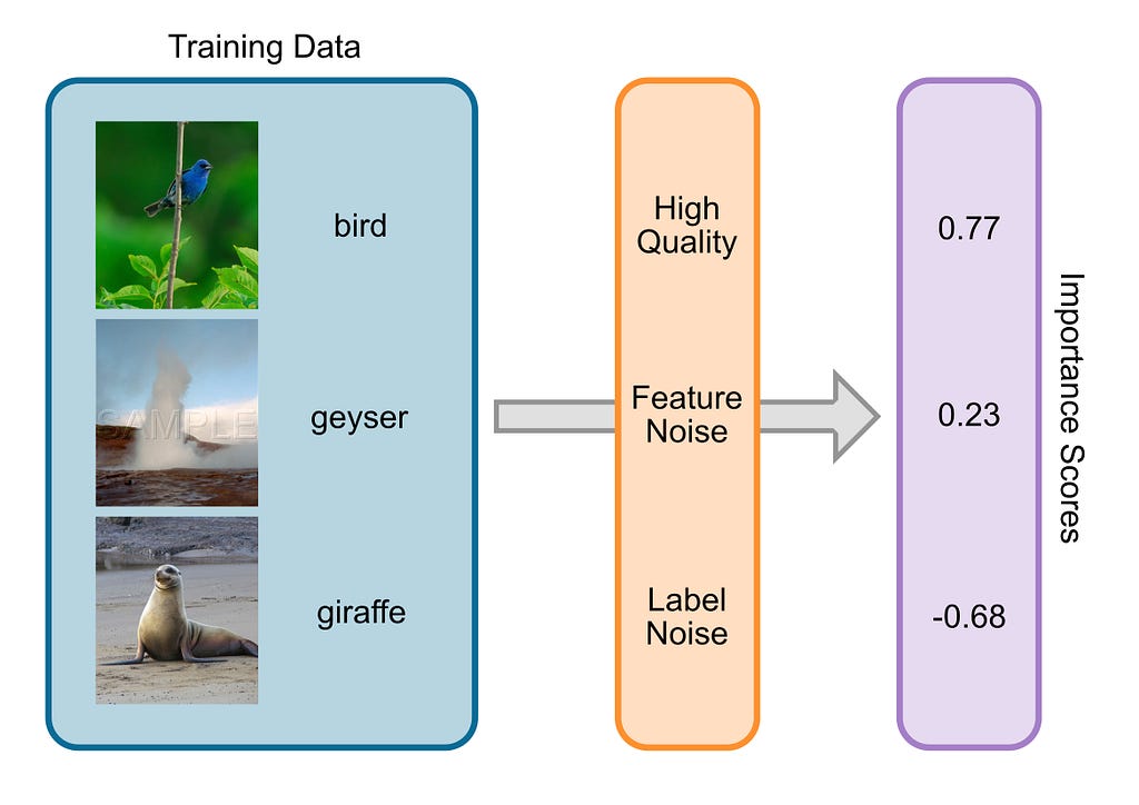
    The process that tries to understand how important different training samples are for the training process of a machine learning model is called Data Valuation. Data Valuation is also known as Data Attribution, Data Influence Analysis, and Representer Points. There are many different approaches and applications, some of which I will discuss in this article.

    Data Valuation visualized. An importance score is assigned to each training sample. (Image by author.)

    Why do we need Data Valuation?

    Data Markets

    AI will become an important economic factor in the coming years, but they are hungry for data. High-quality data is indispensable for training AI models, making it a valuable commodity. This leads to the concept of data markets, where buyers and sellers can trade data for money. Data Valuation is the basis for pricing the data, but there’s a catch: Sellers don’t want to keep their data private until someone buys it, but for buyers, it is hard to understand how important the data of that seller will be without having seen it. To dive deeper into this topic, consider having a look at the papers “A Marketplace for Data: An Algorithmic Solution” and “A Theory of Pricing Private Data”.

    Data Poisoning

    Data poisoning poses a threat to AI models: Bad actors could try to corrupt training data in a way to harm the machine learning training process. This can be done by subtly changing training samples in a way that’s invisible for humans, but very harmful for AI models. Data Valuation methods can counter this because they naturally assign a very low importance score to harmful samples (no matter if they occur naturally, or by malice).

    Explainability

    In recent years, explainable AI has gained a lot of traction. The High-Level Experts Group on AI of the EU even calls for the explainability of AI as foundational for creating trustworthy AI. Understanding how important different training samples are for an AI system or a specific prediction of an AI system is important for explaining its behaviour.

    Active Learning

    If we can better understand how important which training samples of a machine learning model are, then we can use this method to acquire new training samples that are more informative for our model. Say, you are training a new large language model and find out that articles from the Portuguese Wikipedia page are super important for your LLM. Then it’s a natural next step to try to acquire more of those articles for your model. In a similar fashion, we used Data Valuation in our paper on “LossVal” to acquire new vehicle crash tests to improve the passive safety systems of cars.

    Overview of Data Valuation Methods

    Now we know how useful Data Valuation is for different applications. Next, we will have a look at understanding how Data Valuation works. As described in our paper, Data Valuation methods can be roughly divided into three branches:

    • Retraining-Based Approaches
    • Gradient-Based Approaches
    • Data-Based Approaches
    • “Others”

    Retraining-Based Approaches

    The common scheme of retraining-based approaches is that they train a machine learning model multiple times to gain insight into the training dynamics of the model, and ultimately, into the importance of each training sample. The most basic approach (which was introduced in 1977 by Dennis Cook) simply retrains the machine learning model without a data point to determine the importance of that point. If removing the data point decreases the performance of the machine learning model on a validation dataset, then we know that the data point was bad for the model. Reversely, we know that the data point was good (or informative) for the model if the model’s performance on the validation set increases. Repeat the retraining for each data point, and you have valuable importance scores for your complete dataset. This kind of score is called the Leave-One-Out error (LOO). Completely retraining your machine learning model for every single data point is very inefficient, but viable for simple models and small datasets.

    Data Shapley extends this idea using the Shapley value. The idea was published concurrently by both Ghorbani & Zou and by Jia et al. in 2019. The Shapley value is a construct from game theory that tells you how much each player of a coalition contributed to the payout. A closer-to-life example is the following: Imagine you share a Taxi with your friends Bob and Alice on the way home from a party. Alice lives very close to your starting destination, but Bob lives much farther away, and you’re somewhere in between. Of course, it wouldn’t be fair if each of you pays an equal share of the final price, even though you and Bob drive a longer distance than Alice. The Shapley value solves this, by looking at all the sub-coalitions: What if only you and Alice shared the taxi? What if Bob drove alone? And so on. This way, the Shapley value can help you all three pay a fair share towards the final taxi price. This can also be applied to data: Retrain a machine learning model on different subsets of the training data to fairly assign an “importance” to each of the training samples. Unfortunately, this is extremely inefficient: calculating the exact Shapley values would need more than the O(2ⁿ) retrainings of your machine learning model. However, Data Shapley can be approximated much more efficiently using Monte Carlo methods.

    Many alternative methods have been proposed, for example, Data-OOB and Average Marginal Effect (AME). Retraining-based approaches struggle with large training sets, because of the repeated retraining. Importance scores calculated using retraining can be imprecise because of the effect of randomness in neural networks.

    Gradient-Based Approaches

    Gradient-based approaches only work for machine learning algorithms based on gradient, such as Artificial Neural Networks or linear and logistic regression.

    Influence functions are a staple in statistics and were proposed by Dennis Cook, who was mentioned already above. Influence functions use the Hessian matrix (or an approximation of it) to understand how the model’s performance would change if a certain training sample was left out. Using Influence Functions, there is no need to retrain the model. This works for simple regression models, but also for neural networks. Calculating influence functions is quite inefficient, but approximations have been proposed.

    Alternative approaches, like TraceIn and TRAK track the gradient updates during the training of the machine learning model. They can successfully use this information to understand how important a data point is for the training without needing to retrain the model. Gradient Similarity is another method that tracks the gradients but uses them to compare the similarity of training and validation gradients.

    For my master’s thesis, I worked on a new gradient-based Data Valuation method that exploits gradient information in the loss function, called LossVal. We introduced a self-weighting mechanism into standard loss functions like mean squared error and cross-entropy loss. This allows to assign importance scores to training samples during the first training run, making gradient tracking, Hessian matrix calculation, and retraining unnecessary, while still achieving state-of-the-art results.

    Data-Based Approaches

    All methods we touched on above are centered around a machine learning model. This has the advantage, that they tell you how important training samples are for your specific use case and your specific machine learning model. However, some applications (like Data Markets) can profit from “model-agnostic” importance scores that are not based on a specific machine learning model, but instead solely build upon the data.

    This can be done in different ways. For example, one can analyze the distance between the training set and a clean validation set or use a volume measure to quantify the diversity of the data.

    “Others”

    Under this category, I subsume all methods that do not fit into the other categories. For example, using K-nearest neighbors (KNN) allows a much more efficient computation of Shapley values without retraining. Sub-networks that result from zero-masking can be analyzed to understand the importance of different data points. DAVINZ analyzes the change in performance when the training data changes by looking at the generalization boundary. Simfluence runs simulated training runs and can estimate how important each training sample is based on that. Reinforcement learning and evolutionary algorithms can also be used for Data Valuation.

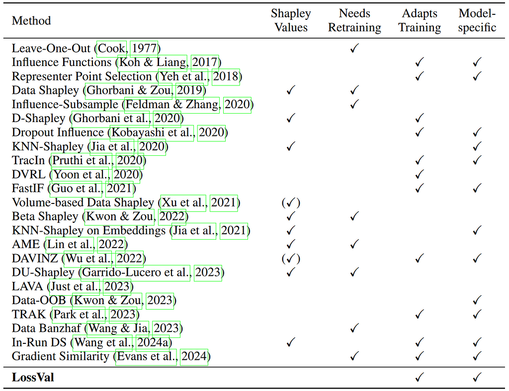
    Overview of some more data valuation methods. (Screenshot from https://arxiv.org/abs/2412.04158)

    Current Research Directions

    Currently, there are some research trends in different directions. Some research is being conducted to bring other game theoretic concepts, like the Banzhaf Value or the Winter value, to Data Valuation. Other approaches try to create joint importance scores that include other aspects of the learning process in the valuation, such as the learning algorithm. Further approaches work on private (where the data does not have to be disclosed) and personalized Data Valuation (where metadata is used to enrich the data).

    Conclusion

    Data Valuation is a growing topic, lots of other Data Valuation methods were not mentioned in this article. Data Valuation is a valuable tool for better understanding and interpreting machine learning models. If you want to learn more about Data Valuation, I can recommend the following articles:


    Data Valuation — A Concise Overview was originally published in Towards Data Science on Medium, where people are continuing the conversation by highlighting and responding to this story.

    Originally appeared here:
    Data Valuation — A Concise Overview

    Go Here to Read this Fast! Data Valuation — A Concise Overview