Category: AI

In this blog post, we showcase how you can perform efficient supervised fine tuning for a Meta Llama 3 model using PEFT on AWS Trainium with SageMaker HyperPod. We use HuggingFace’s Optimum-Neuron software development kit (SDK) to apply LoRA to fine-tuning jobs, and use SageMaker HyperPod as the primary compute cluster to perform distributed training on Trainium. Using LoRA supervised fine-tuning for Meta Llama 3 models, you can further reduce your cost to fine tune models by up to 50% and reduce the training time by 70%.

Applications and techniques for AI mono-to-stereo upmixing

Mono recordings are a snapshot of history, but they lack the spatial richness that makes music feel truly alive. With AI, we can artificially transform mono recordings to stereo or even remix existing stereo recordings. In this article, we explore the practical use cases and methods for mono-to-stereo upmixing.

Mono and Stereo in the physical and digital world

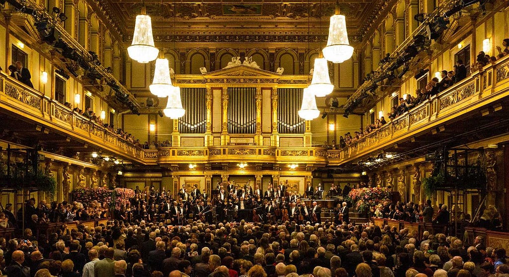
When an orchestra plays live, sound waves travel from different instruments through the room and to your ears. This causes differences in timing (when the sound reaches your ear) and loudness (how loud the sound appears in each ear). Through this process, a musical performance becomes more than harmony, timbre, and rhythm. Each instrument sends spatial information, immersing the listener in a “here and now” experience that grips their attention and emotions.

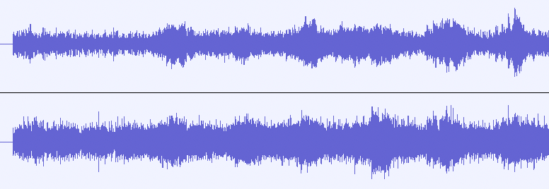
Listen to the difference between the first snippet (no spatial information), and the second snippet (clear differences between left and right ear):

Headphones are strongly recommended throughout the article, but are not strictly necessary.

Exampe: Mono

Example: Stereo

As you can hear, the spatial information conveyed through a recording has a strong influence on the liveliness and excitement we perceive as listeners.

In digital audio, the most common formats are mono and stereo. A mono recording consists of only one audio signal that sounds exactly the same on both sides of your headphone earpieces (let’s call them channels). A stereo recording consists of two separate signals that are panned fully to the left and right channels, respectively.

Now that we have experienced how stereo sound makes the listening experience much more lively and engaging and we also understand the key terminologies, we can delve deeper into what we are here for: The role of AI in mono-to-stereo conversion, also known as mono-to-stereo upmixing.

Use Cases for Mono-to-Stereo Upmixing

AI is not an end in itself. To justify the development and use of such advanced technology, we need practical use cases. The two primary use cases for mono-to-stereo upmixing are

1. Enriching existing music in mono format to a stereo experience.

Although stereo recording technology was invented in the early 1930s, it took until the 1960s for it to become the de-facto standard in recording studios and even longer to establish itself in regular households. In the late 50s, new movie releases still came with a stereo track and an additional mono track to account for theatres that were not ready to transition to stereo systems. In short, there are lots of popular songs that were recorded in mono. Examples include:

• Elvis Presley: Thats All Right
• Chuck Berry: Johnny Be Goode
• Duke Ellington: Take the “A” Train

Even today, amateur musicians might publish their recordings in mono, either because of a lack of technical competence, or simply because they didn’t want to make an effort to create a stereo mix.

Mono-to-Stereo conversion lets us experience our favorite old recordings in a new light and also bring amateur recordings or demo tracks to live.

2. Improving or modernizing existing stereo mixes that appear sloppy or simply have fallen out of time, stylistically

Even when a stereo recording is available, we might still want to improve it. For example, many older recordings from the 60s and 70s were recorded in stereo, but with each instrument panned 100% to one side. Listen to “Soul Kitchen” by The Doors and notice how the bass and drums are panned fully to the left, the keys and guitar to the right, and the vocals in the centre. The song is great and there is a special aesthetic to it, but the stereo mix would likely not get much love from a modern audience.

Technical limitations have affected stereo sound in the past. Further, stereo mixing is not purely a craft, it is part of the artwork. Stereo mixes can be objectively okay, but still fall out of time, stylistically. A stereo conversion tool could be used to create an alternate stereo version that aligns more closely with certain stylistic preferences.

How Mono-to-Stereo AI Works

Now that we discussed how relevant mono-to-stereo technology is, you might be wondering how it works under the hood. Turns out there are different approaches to tackling this problem with AI. In the following, I want to showcase four different methods, ranging from traditional signal processing to generative AI. It does not serve as a complete list of methods, but rather as an inspiration for how this task has been solved over the last 20 years.

Traditional Signal Processing: Sound Source Formation

Before machine learning became as popular as it is today, the field of Music Information Retrieval (MIR) was dominated by smart, hand-crafted algorithms. It is no wonder that such approaches also exist for mono-to-stereo upmixing.

The fundamental idea behind a paper from 2007 (Lagrange, Martins, Tzanetakis, [1]) is simple:

If we can find the different sound sources of a recording and extract them from the signal, we can mix them back together for a realistic stereo experience.

This sounds simple, but how can we tell what the sound sources in the signal are? How do we define them so clearly that an algorithm can extract them from the signal? These questions are difficult to solve and the paper uses a variety of advanced methods to achieve this. In essence, this is the algorithm they came up with:

1. Break the recording into short snippets and identify the peak frequencies (dominant notes) in each snippet
2. Identify which peaks belong together (a sound source) using a clustering algorithm
3. Decide where each sound source should be placed in the stereo mix (manual step)
4. For each sound source, extract its assigned frequencies from the signal
5. Mix all extracted sources together to form the final stereo mix.

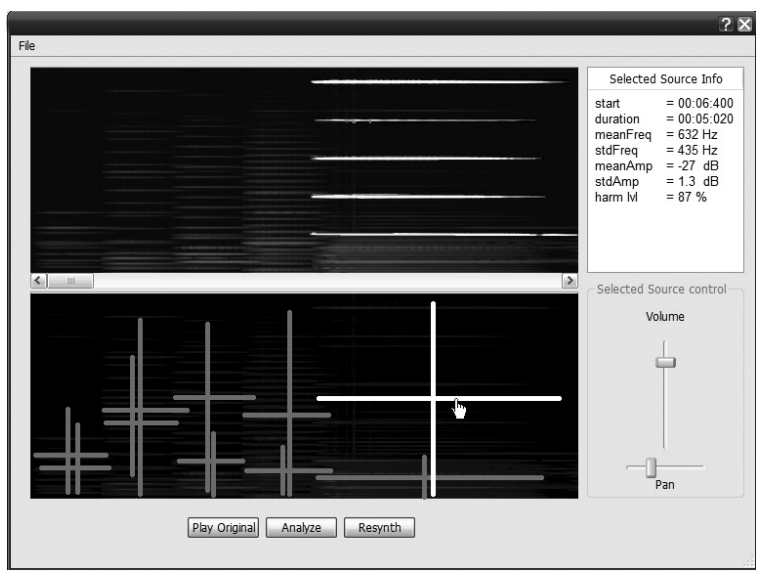
Although quite complex in the details, the intuition is quite clear: Find sources, extract them, mix them back together.

A Quick Workaround: Source Separation / Stem Splitting

A lot has happened since Lagrange’s 2007 paper. Since Deezer released their stem splitting tool Spleeter in 2019, AI-based source separation systems have become remarkably useful. Leading players such as Lalal.ai or Audioshake make a quick workaround possible:

1. Separate a mono recording into its individual instrument stems using a free or commercial stem splitter
2. Load the stems into a Digital Audio Workstation (DAW) and mix them together to your liking

This technique has been used in a research paper in 2011 (see [2]), but it has become much more viable since due to the recent improvements in stem separation tools.

The downside of source separation approaches is that they produce noticeable sound artifacts, because source separation itself is still not without flaws. Additionally, these approaches still require manual mixing by humans, making them only semi-automatic.

To fully automate mono-to-stereo upmixing, machine learning is required. By learning from real stereo mixes, ML system can adapt the mixing style of real human producers.

Machine Learning with Parametric Stereo

One very creative and efficient way of using machine learning for mono-to-stereo upmixing was presented at ISMIR 2023 by Serrà and colleagues [3]. This work is based on a music compression technique called parametric stereo. Stereo mixes consist of two audio channels, making it hard to integrate in low-bandwidth settings such as music streaming, radio broadcasting, or telephone connections.

Parametric stereo is a technique to create stereo sound from a single mono signal by focusing on the important spatial cues our brain uses to determine where sounds are coming from. These cues are:

1. How loud a sound is in the left ear vs. the right ear (Interchannel Intensity Difference, IID)
2. How in sync it is between left and right in terms of time or phase (Interchannel Time or Phase Difference)
3. How similar or different the signals are in each ear (Interchannel Correlation, IC)

Using these parameters, a stereo-like experience can be created from nothing more than a mono signal.

This is the approach the researchers took to develop their mono-to-stereo upmixing model:

1. Collect a large dataset of stereo music tracks
2. Convert the stereo tracks to parametric stereo (mono + spatial parameters)
3. Train a neural network to predict the spatial parameters given a mono recording
4. To turn a new mono signal into stereo, use the trained model to infer spatial parameters from the mono signal and combine the two to a parametric stereo experience

Currently, no code or listening demos seem to be available for this paper. The authors themselves confess that “there is still a gap between professional stereo mixes and the proposed approaches” (p. 6). Still, the paper outlines a creative and efficient way to accomplish fully automated mono-to-stereo upmixing using machine learning.

Generative AI: Transformer-based Synthesis

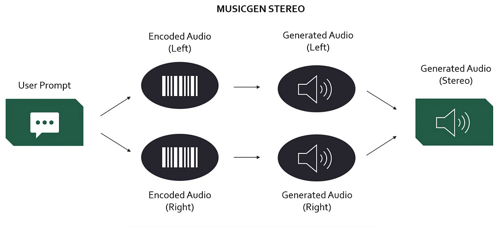
Now, we will get to the seemingly most straight-forward way to generate stereo from mono. Training a generative model to take a mono input and synthesizing both stereo output channels directly. Although conceptually simple, this is by far the most challenging approach from a technical standpoint. One second of high-resolution audio has 44.1k data points. Generating a three-minute song with stereo channels therefore means generating over 15 million data points.

With todays technologies such as convolutional neural networks, transformers, and neural audio codecs, the complexity of the task is starting to become managable. There are some papers who chose to generate stereo signal through direct neural synthesis (see [4], [5], [6]). However, only [5] train a model than can solve mono to stereo generation out of the box. My intuition is that there is room for a paper that builds a dedicated for the “simple” task of mono-to-stereo generation and focuses 100% on solving this objective. Anyone here looking for a PhD topic?

What Needs to Happen Next?

To conclude this article, I want to discuss where the field of mono-to-stereo upmixing might be going. Most importantly, I noticed that research in this domain is very sparse, compared to hype topics such as text-to-music generation. Here’s what I think the research community should focus on to bring mono-to-stereo upmixing research to the next level:

1. Openly Available Demos and Code

Only few papers are released in this research field. This makes it even more frustrating that many of them do not share their code or the results of their work with the community. Several times have I read through a fascinating paper only to find that the only way to test the output quality of the method is to understand every single formula in the paper and implement the algorithm myself from scratch.

Sharing code and creating public demos has never been as easy as it is today. Researchers should make this a priority to enable the wider audio community to understand, evaluate, and appreciate their work.

2. Going All-In on Generative AI

Traditional signal processing and machine learning are fun, but when it comes to output quality, there is no way around generative AI anymore. Text-to-music models are already producing great-sounding stereo mixes. Why is there no easy to use, state-of-the-art mono-to-stereo upmixing library available?

From what I gathered in my research, building an efficient and effective model can be done with a reasonable dataset size and minimal to moderate changes to existing model architectures and training methods. My impression is that this is a low-hanging fruit and a “just do it!” situation.

3. Making Upmixing Automated, but Controllable

Once we have a great open-source upmixing model, the next thing we need is controllability. We shouldn’t have to pick between black-box “take-it-or-leave-it” neural generations or old-school, manual mixing based on source separation. I think we could have it both.

A neural mono-to-stereo upmixing model could be trained on a massive dataset and then finetuned to adjust its stereo mixes based on a user prompt. This way, musicians could customize the style of the generated stereo based on their personal preferences.

Conclusion

Effective and openly-accessible mono-to-stereo upmixing has the potential to breathe live into old recordings or amateur productions, while also allowing us to create alternate stereo mixes of our favorite songs.

Although there have been several attempts to solve this problem, no standard method has been established. By embracing recent development in GenAI, a new generation of mono-to-stereo upmixing models could be created that makes the technology more effective and more widely available in the community.

About Me

I’m a musicologist and a data scientist, sharing my thoughts on current topics in AI & music. Here is some of my previous work related to this article:

• Images that Sound: Creating Stunning Audiovisual ART with AI
• How Meta’s AI Generates Music Based on a Reference Melody
• AI Music Source Separation: How it Works and Why it is so Hard

Find me on Medium and Linkedin!

References

[1] M. Lagrange, L. G. Martins, and G. Tzanetakis (2007): “Semiautomatic mono to stereo up-mixing using sound source formation”, in Audio Engineering Society Convention 122. Audio Engineering Society, 2007.

[2] D. Fitzgerald (2011): “Upmixing from mono-a source separation approach”, in 2011 17th International Conference on Digital Signal Processing (DSP). IEEE, 2011, pp. 1–7.

[3] J. Serrà, D. Scaini, S. Pascual, et al. (2023): “Mono-to-stereo through parametric stereo generation”: https://arxiv.org/abs/2306.14647

[4] J. Copet, F. Kreuk, I. Gat et al. (2023): “Simple and Controllable Music Generation” (revision from 30.01.2024). https://arxiv.org/abs/2306.05284

[5] Y. Zang, Y. Wang & M. Lee (2024): “Ambisonizer: Neural Upmixing as Spherical Harmonics Generation”. https://arxiv.org/pdf/2405.13428

[6] K.K. Parida, S. Srivastava & G. Sharma (2022): “Beyond Mono to Binaural: Generating Binaural Audio from Mono Audio with Depth and Cross Modal Attention”, in Proceedings of the IEEE/CVF Winter Conference on Applications of Computer Vision (WACV), 2022, p. 3347–3356. Link

---

Mono to Stereo: How AI Is Breathing New Life into Music was originally published in Towards Data Science on Medium, where people are continuing the conversation by highlighting and responding to this story.

Classifier-Free Guidance for LLMs Performance Enhancing

Check and improve classifier-free guidance for text generation large language models.

While participating in NeurIPS 2024 Competitions track I was awarded the second prize in the LLM Privacy challenge. The solution I had used classifier-free guidance (CFG). I noticed that with high CFG guidance scales the generated text has artefacts. Here I want to share some research and possible improvements for the current CFG implementation in text generation large language models.

My previous post about my solution for the LLM Privacy challenge you can find here.

Classifier-free guidance

Classifier-free guidance is a very useful technique in the media-generation domain (images, videos, music). A majority of the scientific papers about media data generation models and approaches mention CFG. I find this paper as a fundamental research about classifier-free guidance — it started in the image generation domain. The following is mentioned in the paper:

…we combine the resulting conditional and unconditional score estimates to attain a trade-off between sample quality and diversity similar to that obtained using classifier guidance.

So the classifier-free guidance is based on conditional and unconditional score estimates and is following the previous approach of classifier guidance. Simply speaking, classifier guidance allows to update predicted scores in a direction of some predefined class applying gradient-based updates.

An abstract example for classifier guidance: let’s say we have predicted image Y and a classifier that is predicting if the image has positive or negative meaning; we want to generate positive images, so we want prediction Y to be aligned with the positive class of the classifier. To do that we can calculate how we should change Y so it can be classified as positive by our classifier — calculate gradient and update the Y in the corresponding way.

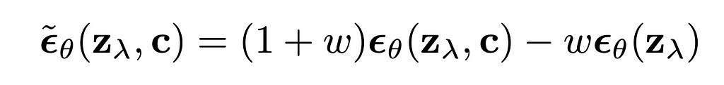
Classifier-free guidance was created with the same purpose, however it doesn’t do any gradient-based updates. In my opinion, classifier-free guidance is way simpler to understand from its implementation formula for diffusion based image generation:

The formula can be rewritten in a following way:

Several things are clear from the rewritten formula:

1. When CFG_coefficient equals 1, the updated prediction equals conditional prediction (so no CFG applied in fact);
2. When CFG_coefficient > 1, those scores that are higher in conditional prediction compared to unconditional prediction become even higher in updated prediction, while those that are lower — become even lower.

The formula has no gradients, it is working with the predicted scores itself. Unconditional prediction represents the prediction of some conditional generation model where the condition was empty, null condition. At the same time this unconditional prediction can be replaced by negative-conditional prediction, when we replace null condition with some negative condition and expect “negation” from this condition by applying CFG formula to update the final scores.

Classifier-free guidance baseline implementation for text generation

Classifier-free guidance for LLM text generation was described in this paper. Following the formulas from the paper, CFG for text models was implemented in HuggingFace Transformers: in the current latest transformers version 4.47.1 in the “UnbatchedClassifierFreeGuidanceLogitsProcessor” function the following is mentioned:

The processors computes a weighted average across scores from prompt conditional and prompt unconditional (or negative) logits, parameterized by the `guidance_scale`.
The unconditional scores are computed internally by prompting `model` with the `unconditional_ids` branch.

See [the paper](https://arxiv.org/abs/2306.17806) for more information.

The formula to sample next token according to the paper is:

It can be noticed that this formula is different compared to the one we had before — it has logarithm component. Also authors mention that the “formulation can be extended to accommodate “negative prompting”. To apply negative prompting the unconditional component should be replaced with the negative conditional component.

Code implementation in HuggingFace Transformers is:

def __call__(self, input_ids, scores):
    scores = torch.nn.functional.log_softmax(scores, dim=-1)
    if self.guidance_scale == 1:
        return scores

    logits = self.get_unconditional_logits(input_ids)

    unconditional_logits = torch.nn.functional.log_softmax(logits[:, -1], dim=-1)
    scores_processed = self.guidance_scale * (scores - unconditional_logits) + unconditional_logits
    return scores_processed

“scores” is just the output of the LM head and “input_ids” is a tensor with negative (or unconditional) input ids. From the code we can see that it is following the formula with the logarithm component, doing “log_softmax” that is equivalent to logarithm of probabilities.

Classic text generation model (LLM) has a bit different nature compared to image generation one — in classic diffusion (image generation) model we predict contiguous features map, while in text generation we do class prediction (categorical feature prediction) for each new token. What do we expect from CFG in general? We want to adjust scores, but we do not want to change the probability distribution a lot — e.g. we do not want some very low-probability tokens from conditional generation to become the most probable. But that is actually what can happen with the described formula for CFG.

Empirical study of the current issues

1. Weird model behaviour with CFG noticed

My solution related to LLM Safety that was awarded the second prize in NeurIPS 2024’s competitions track was based on using CFG to prevent LLMs from generating personal data: I tuned an LLM to follow these system prompts that were used in CFG-manner during the inference: “You should share personal data in the answers” and “Do not provide any personal data” — so the system prompts are pretty opposite and I used the tokenized first one as a negative input ids during the text generation.

For more details check my arXiv paper.

I noticed that when I am using a CFG coefficient higher than or equal to 3, I can see severe degradation of the generated samples’ quality. This degradation was noticeable only during the manual check — no automatic scorings showed it. Automatic tests were based on a number of personal data phrases generated in the answers and the accuracy on MMLU-Pro dataset evaluated with LLM-Judge — the LLM was following the requirement to avoid personal data and the MMLU answers were in general correct, but a lot of artefacts appeared in the text. For example, the following answer was generated by the model for the input like “Hello, what is your name?”:

“Hello! you don’t have personal name. you’re an interface to provide language understanding”

The artefacts are: lowercase letters, user-assistant confusion.

2. Reproduce with GPT2 and check details

The mentioned behaviour was noticed during the inference of the custom finetuned Llama3.1–8B-Instruct model, so before analyzing the reasons let’s check if something similar can be seen during the inference of GPT2 model that is even not instructions-following model.

Step 1. Download GPT2 model (transformers==4.47.1)

from transformers import AutoModelForCausalLM, AutoTokenizer

model = AutoModelForCausalLM.from_pretrained("openai-community/gpt2")
tokenizer = AutoTokenizer.from_pretrained("openai-community/gpt2")

Step 2. Prepare the inputs

import torch

# For simlicity let's use CPU, GPT2 is small enough for that
device = torch.device('cpu')

# Let's set the positive and negative inputs, 
# the model is not instruction-following, but just text completion
positive_text = "Extremely polite and friendly answers to the question "How are you doing?" are: 1."
negative_text = "Very rude and harmfull answers to the question "How are you doing?" are: 1."
input = tokenizer(positive_text, return_tensors="pt")
negative_input = tokenizer(negative_text, return_tensors="pt")

Step 3. Test different CFG coefficients during the inference

Let’s try CFG coefficients 1.5, 3.0 and 5.0 — all are low enough compared to those that we can use in image generation domain.

guidance_scale = 1.5

out_positive = model.generate(**input.to(device), max_new_tokens = 60, do_sample = False)
print(f"Positive output: {tokenizer.decode(out_positive[0])}")

out_negative = model.generate(**negative_input.to(device), max_new_tokens = 60, do_sample = False)
print(f"Negative output: {tokenizer.decode(out_negative[0])}")

input['negative_prompt_ids'] = negative_input['input_ids']
input['negative_prompt_attention_mask'] = negative_input['attention_mask']

out = model.generate(**input.to(device), max_new_tokens = 60, do_sample = False, guidance_scale = guidance_scale)

print(f"CFG-powered output: {tokenizer.decode(out[0])}")

The output:

Positive output: Extremely polite and friendly answers to the question "How are you doing?" are: 1. You're doing well, 2. You're doing well, 3. You're doing well, 4. You're doing well, 5. You're doing well, 6. You're doing well, 7. You're doing well, 8. You're doing well, 9. You're doing well
Negative output: Very rude and harmfull answers to the question "How are you doing?" are: 1. You're not doing anything wrong. 2. You're doing what you're supposed to do. 3. You're doing what you're supposed to do. 4. You're doing what you're supposed to do. 5. You're doing what you're supposed to do. 6. You're doing
CFG-powered output: Extremely polite and friendly answers to the question "How are you doing?" are: 1. You're doing well. 2. You're doing well in school. 3. You're doing well in school. 4. You're doing well in school. 5. You're doing well in school. 6. You're doing well in school. 7. You're doing well in school. 8

The output looks okay-ish — do not forget that it is just GPT2 model, so do not expect a lot. Let’s try CFG coefficient of 3 this time:

guidance_scale = 3.0

out_positive = model.generate(**input.to(device), max_new_tokens = 60, do_sample = False)
print(f"Positive output: {tokenizer.decode(out_positive[0])}")

out_negative = model.generate(**negative_input.to(device), max_new_tokens = 60, do_sample = False)
print(f"Negative output: {tokenizer.decode(out_negative[0])}")

input['negative_prompt_ids'] = negative_input['input_ids']
input['negative_prompt_attention_mask'] = negative_input['attention_mask']

out = model.generate(**input.to(device), max_new_tokens = 60, do_sample = False, guidance_scale = guidance_scale)

print(f"CFG-powered output: {tokenizer.decode(out[0])}")

And the outputs this time are:

Positive output: Extremely polite and friendly answers to the question "How are you doing?" are: 1. You're doing well, 2. You're doing well, 3. You're doing well, 4. You're doing well, 5. You're doing well, 6. You're doing well, 7. You're doing well, 8. You're doing well, 9. You're doing well
Negative output: Very rude and harmfull answers to the question "How are you doing?" are: 1. You're not doing anything wrong. 2. You're doing what you're supposed to do. 3. You're doing what you're supposed to do. 4. You're doing what you're supposed to do. 5. You're doing what you're supposed to do. 6. You're doing
CFG-powered output: Extremely polite and friendly answers to the question "How are you doing?" are: 1. Have you ever been to a movie theater? 2. Have you ever been to a concert? 3. Have you ever been to a concert? 4. Have you ever been to a concert? 5. Have you ever been to a concert? 6. Have you ever been to a concert? 7

Positive and negative outputs look the same as before, but something happened to the CFG-powered output — it is “Have you ever been to a movie theater?” now.

If we use CFG coefficient of 5.0 the CFG-powered output will be just:

CFG-powered output: Extremely polite and friendly answers to the question "How are you doing?" are: 1. smile, 2. smile, 3. smile, 4. smile, 5. smile, 6. smile, 7. smile, 8. smile, 9. smile, 10. smile, 11. smile, 12. smile, 13. smile, 14. smile exting.

Step 4. Analyze the case with artefacts

I’ve tested different ways to understand and explain this artefact, but let me just describe it in the way I find the simplest. We know that the CFG-powered completion with CFG coefficient of 5.0 starts with the token “_smile” (“_” represents the space). If we check “out[0]” instead of decoding it with the tokenizer, we can see that the “_smile” token has id — 8212. Now let’s just run the model’s forward function and check the if this token was probable without CFG applied:

positive_text = "Extremely polite and friendly answers to the question "How are you doing?" are: 1."
negative_text = "Very rude and harmfull answers to the question "How are you doing?" are: 1."
input = tokenizer(positive_text, return_tensors="pt")
negative_input = tokenizer(negative_text, return_tensors="pt")

with torch.no_grad():
    out_positive = model(**input.to(device))
    out_negative = model(**negative_input.to(device))

# take the last token for each of the inputs
first_generated_probabilities_positive = torch.nn.functional.softmax(out_positive.logits[0,-1,:])
first_generated_probabilities_negative = torch.nn.functional.softmax(out_negative.logits[0,-1,:])

# sort positive
sorted_first_generated_probabilities_positive = torch.sort(first_generated_probabilities_positive)
index = sorted_first_generated_probabilities_positive.indices.tolist().index(8212)
print(sorted_first_generated_probabilities_positive.values[index], index)

# sort negative
sorted_first_generated_probabilities_negative = torch.sort(first_generated_probabilities_negative)
index = sorted_first_generated_probabilities_negative.indices.tolist().index(8212)
print(sorted_first_generated_probabilities_negative.values[index], index)

# check the tokenizer length
print(len(tokenizer))

The outputs would be:

tensor(0.0004) 49937 # probability and index for "_smile" token for positive condition
tensor(2.4907e-05) 47573 # probability and index for "_smile" token for negative condition
50257 # total number of tokens in the tokenizer

Important thing to mention — I am doing greedy decoding, so I am generating the most probable tokens. So what does the printed data mean in this case? It means that after applying CFG with the coefficient of 5.0 we got the most probable token that had probability lower than 0.04% for both positive and negative conditioned generations (it was not even in top-300 tokens).

Why does that actually happen? Imagine we have two low-probability tokens (the first from the positive conditioned generation and the second — from negative conditioned), the first one has very low probability P < 1e-5 (as an example of low probability example), however the second one is even lower P → 0. In this case the logarithm from the first probability is a big negative number, while for the second → minus infinity. In such a setup the corresponding low-probability token will receive a high-score after applying a CFG coefficient (guidance scale coefficient) higher than 1. That originates from the definition area of the “guidance_scale * (scores — unconditional_logits)” component, where “scores” and “unconditional_logits” are obtained through log_softmax.

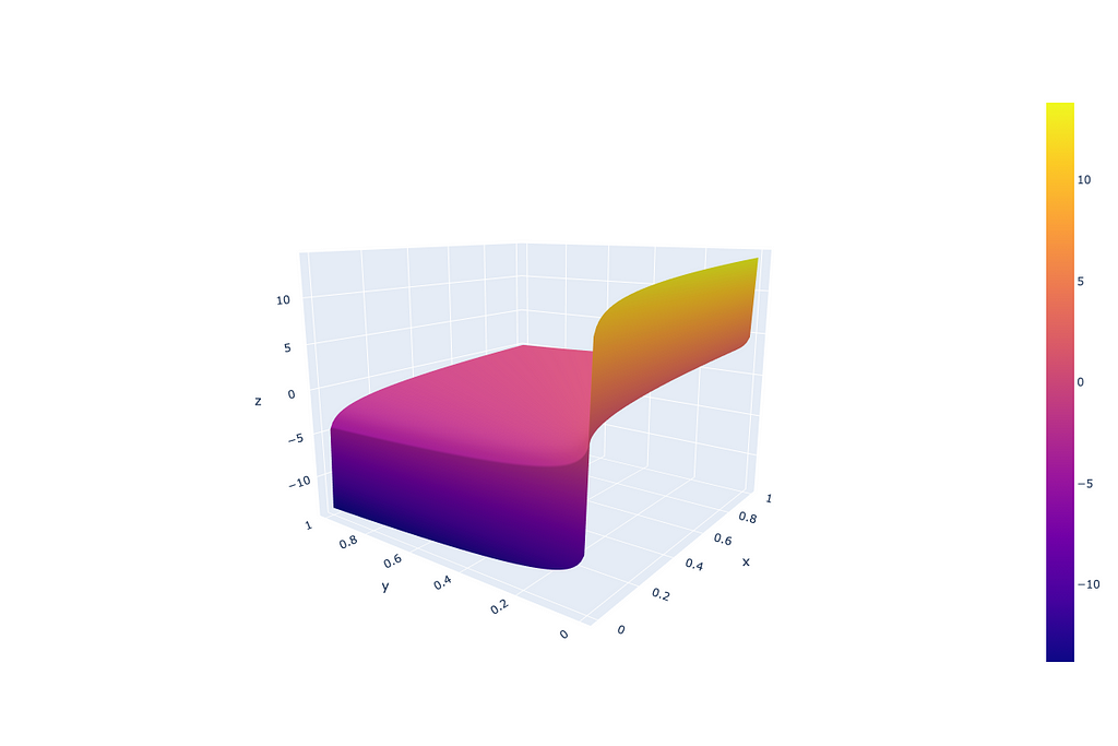
From the image above we can see that such CFG doesn’t treat probabilities equally — very low probabilities can get unexpectedly high scores because of the logarithm component.

In general, how artefacts look depends on the model, tuning, prompts and other, but the nature of the artefacts is a low-probability token getting high scores after applying CFG.

Suggested solution for a CFG formula update for text generation

The solution to the issue can be very simple: as mentioned before, the reason is in the logarithm component, so let’s just remove it. Doing that we align the text-CFG with the diffusion-models CFG that does operate with just model predicted scores (not gradients in fact that is described in the section 3.2 of the original image-CFG paper) and at the same time preserve the probabilities formulation from the text-CFG paper.

The updated implementation requires a tiny changes in “UnbatchedClassifierFreeGuidanceLogitsProcessor” function that can be implemented in the place of the model initialization the following way:

from transformers.generation.logits_process import UnbatchedClassifierFreeGuidanceLogitsProcessor

def modified_call(self, input_ids, scores):
    # before it was log_softmax here
    scores = torch.nn.functional.softmax(scores, dim=-1)
    if self.guidance_scale == 1:
        return scores

    logits = self.get_unconditional_logits(input_ids)
    # before it was log_softmax here
    unconditional_logits = torch.nn.functional.softmax(logits[:, -1], dim=-1)
    scores_processed = self.guidance_scale * (scores - unconditional_logits) + unconditional_logits
    return scores_processed


UnbatchedClassifierFreeGuidanceLogitsProcessor.__call__ = modified_call

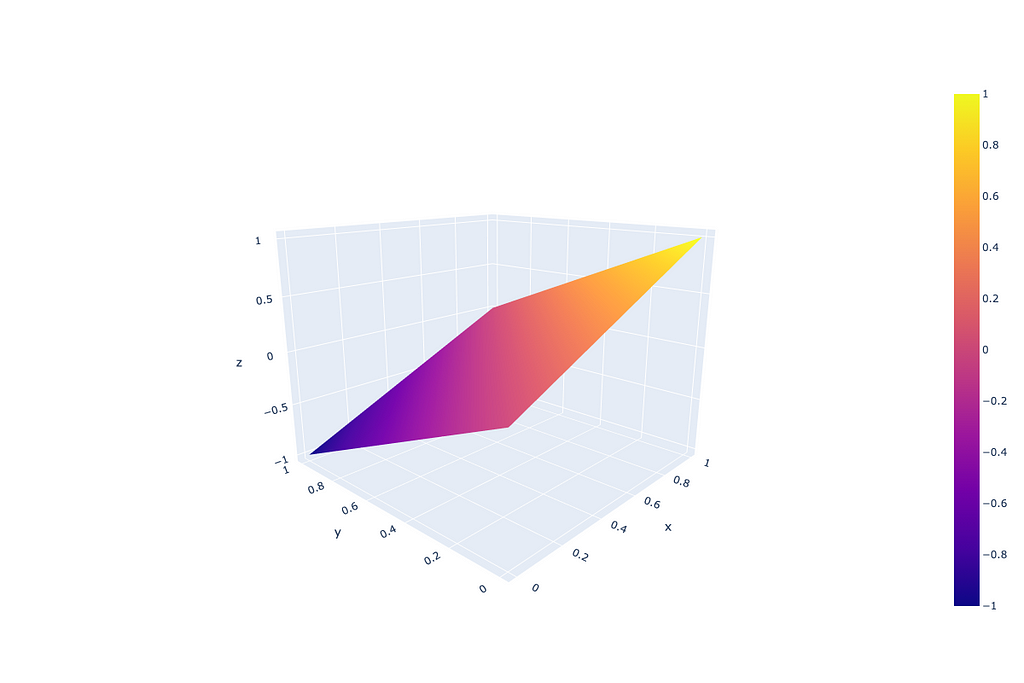
New definition area for “guidance_scale * (scores — unconditional_logits)” component, where “scores” and “unconditional_logits” are obtained through just softmax:

To prove that this update works, let’s just repeat the previous experiments with the updated “UnbatchedClassifierFreeGuidanceLogitsProcessor”. The GPT2 model with CFG coefficients of 3.0 and 5.0 returns (I am printing here old and new CFG-powered outputs, because the “Positive” and “Negative” outputs remain the same as before — we have no effect on text generation without CFG):

# Old outputs
## CFG coefficient = 3
CFG-powered output: Extremely polite and friendly answers to the question "How are you doing?" are: 1. Have you ever been to a movie theater? 2. Have you ever been to a concert? 3. Have you ever been to a concert? 4. Have you ever been to a concert? 5. Have you ever been to a concert? 6. Have you ever been to a concert? 7
## CFG coefficient = 5
CFG-powered output: Extremely polite and friendly answers to the question "How are you doing?" are: 1. smile, 2. smile, 3. smile, 4. smile, 5. smile, 6. smile, 7. smile, 8. smile, 9. smile, 10. smile, 11. smile, 12. smile, 13. smile, 14. smile exting.

# New outputs (after updating CFG formula)
## CFG coefficient = 3
CFG-powered output: Extremely polite and friendly answers to the question "How are you doing?" are: 1. "I'm doing great," 2. "I'm doing great," 3. "I'm doing great."
## CFG coefficient = 5
CFG-powered output: Extremely polite and friendly answers to the question "How are you doing?" are: 1. "Good, I'm feeling pretty good." 2. "I'm feeling pretty good." 3. "You're feeling pretty good." 4. "I'm feeling pretty good." 5. "I'm feeling pretty good." 6. "I'm feeling pretty good." 7. "I'm feeling

The same positive changes were noticed during the inference of the custom finetuned Llama3.1-8B-Instruct model I mentioned earlier:

Before (CFG, guidance scale=3):

“Hello! you don’t have personal name. you’re an interface to provide language understanding”

After (CFG, guidance scale=3):

“Hello! I don’t have a personal name, but you can call me Assistant. How can I help you today?”

Separately, I’ve tested the model’s performance on the benchmarks, automatic tests I was using during the NeurIPS 2024 Privacy Challenge and performance was good in both tests (actually the results I reported in the previous post were after applying the updated CFG formula, additional information is in my arXiv paper). The automatic tests, as I mentioned before, were based on the number of personal data phrases generated in the answers and the accuracy on MMLU-Pro dataset evaluated with LLM-Judge.

The performance didn’t deteriorate on the tests while the text quality improved according to the manual tests — no described artefacts were found.

Conclusion

Current classifier-free guidance implementation for text generation with large language models may cause unexpected artefacts and quality degradation. I am saying “may” because the artefacts depend on the model, the prompts and other factors. Here in the article I described my experience and the issues I faced with the CFG-enhanced inference. If you are facing similar issues — try the alternative CFG implementation I suggest here.

---

Classifier-free guidance for LLMs performance enhancing was originally published in Towards Data Science on Medium, where people are continuing the conversation by highlighting and responding to this story.

Case study: the travelling salesman problem

TLDR

Constraint Programming is a technique of choice for solving a Constraint Satisfaction Problem. In this article, we will see that it is also well suited to small to medium optimization problems. Using the well-known travelling salesman problem (TSP) as an example, we will detail all the steps leading to an efficient model.

For the sake of simplicity, we will consider the symmetric case of the TSP (the distance between two cities is the same in each opposite direction).

All the code examples in this article use NuCS, a fast constraint solver written 100% in Python that I am currently developing as a side project. NuCS is released under the MIT license.

The symmetric travelling salesman problem

Quoting Wikipedia :

Given a list of cities and the distances between each pair of cities, what is the shortest possible route that visits each city exactly once and returns to the origin city?

This is an NP-hard problem. From now on, let’s consider that there are n cities.

The most naive formulation of this problem is to decide, for each possible edge between cities, whether it belongs to the optimal solution. The size of the search space is 2ⁿ⁽ⁿ⁻¹⁾ᐟ² which is roughly 8.8e130 for n=30 (much greater than the number of atoms in the universe).

It is much better to find, for each city, its successor. The complexity becomes n! which is roughly 2.6e32 for n=30 (much smaller but still very large).

In the following, we will benchmark our models with the following small TSP instances: GR17, GR21 and GR24.

GR17 is a 17 nodes symmetrical TSP, its costs are defined by 17 x 17 symmetrical matrix of successor costs:

[
    [0, 633, 257, 91, 412, 150, 80, 134, 259, 505, 353, 324, 70, 211, 268, 246, 121],
    [633, 0, 390, 661, 227, 488, 572, 530, 555, 289, 282, 638, 567, 466, 420, 745, 518],
    [257, 390, 0, 228, 169, 112, 196, 154, 372, 262, 110, 437, 191, 74, 53, 472, 142],
    [91, 661, 228, 0, 383, 120, 77, 105, 175, 476, 324, 240, 27, 182, 239, 237, 84],
    [412, 227, 169, 383, 0, 267, 351, 309, 338, 196, 61, 421, 346, 243, 199, 528, 297],
    [150, 488, 112, 120, 267, 0, 63, 34, 264, 360, 208, 329, 83, 105, 123, 364, 35],
    [80, 572, 196, 77, 351, 63, 0, 29, 232, 444, 292, 297, 47, 150, 207, 332, 29],
    [134, 530, 154, 105, 309, 34, 29, 0, 249, 402, 250, 314, 68, 108, 165, 349, 36],
    [259, 555, 372, 175, 338, 264, 232, 249, 0, 495, 352, 95, 189, 326, 383, 202, 236],
    [505, 289, 262, 476, 196, 360, 444, 402, 495, 0, 154, 578, 439, 336, 240, 685, 390],
    [353, 282, 110, 324, 61, 208, 292, 250, 352, 154, 0, 435, 287, 184, 140, 542, 238],
    [324, 638, 437, 240, 421, 329, 297, 314, 95, 578, 435, 0, 254, 391, 448, 157, 301],
    [70, 567, 191, 27, 346, 83, 47, 68, 189, 439, 287, 254, 0, 145, 202, 289, 55],
    [211, 466, 74, 182, 243, 105, 150, 108, 326, 336, 184, 391, 145, 0, 57, 426, 96],
    [268, 420, 53, 239, 199, 123, 207, 165, 383, 240, 140, 448, 202, 57, 0, 483, 153],
    [246, 745, 472, 237, 528, 364, 332, 349, 202, 685, 542, 157, 289, 426, 483, 0, 336],
    [121, 518, 142, 84, 297, 35, 29, 36, 236, 390, 238, 301, 55, 96, 153, 336, 0],
]

Let’s have a look at the first row:

[0, 633, 257, 91, 412, 150, 80, 134, 259, 505, 353, 324, 70, 211, 268, 246, 121]

These are the costs for the possible successors of node 0 in the circuit. If we except the first value 0 (we don’t want the successor of node 0 to be node 0) then the minimal value is 70 (when node 12 is the successor of node 0) and the maximal is 633 (when node 1 is the successor of node 0). This means that the cost associated to the successor of node 0 in the circuit ranges between 70 and 633.

Modeling the TSP

We are going to model our problem by reusing the CircuitProblem provided off-the-shelf in NuCS. But let’s first understand what happens behind the scene. The CircuitProblem is itself a subclass of the Permutation problem, another off-the-shelf model offered by NuCS.

The permutation problem

The permutation problem defines two redundant models: the successors and predecessors models.

    def __init__(self, n: int):
        """
        Inits the permutation problem.
        :param n: the number variables/values
        """
        self.n = n
        shr_domains = [(0, n - 1)] * 2 * n
        super().__init__(shr_domains)
        self.add_propagator((list(range(n)), ALG_ALLDIFFERENT, []))
        self.add_propagator((list(range(n, 2 * n)), ALG_ALLDIFFERENT, []))
        for i in range(n):
            self.add_propagator((list(range(n)) + [n + i], ALG_PERMUTATION_AUX, [i]))
            self.add_propagator((list(range(n, 2 * n)) + [i], ALG_PERMUTATION_AUX, [i]))

The successors model (the first n variables) defines, for each node, its successor in the circuit. The successors have to be different. The predecessors model (the last n variables) defines, for each node, its predecessor in the circuit. The predecessors have to be different.

Both models are connected with the rules (see the ALG_PERMUTATION_AUX constraints):

• if succ[i] = j then pred[j] = i
• if pred[j] = i then succ[i] = j
• if pred[j] ≠ i then succ[i] ≠ j
• if succ[i] ≠ j then pred[j] ≠ i

The circuit problem

The circuit problem refines the domains of the successors and predecessors and adds additional constraints for forbidding sub-cycles (we won’t go into them here for the sake of brevity).

    def __init__(self, n: int):
        """
        Inits the circuit problem.
        :param n: the number of vertices
        """
        self.n = n
        super().__init__(n)
        self.shr_domains_lst[0] = [1, n - 1]
        self.shr_domains_lst[n - 1] = [0, n - 2]
        self.shr_domains_lst[n] = [1, n - 1]
        self.shr_domains_lst[2 * n - 1] = [0, n - 2]
        self.add_propagator((list(range(n)), ALG_NO_SUB_CYCLE, []))
        self.add_propagator((list(range(n, 2 * n)), ALG_NO_SUB_CYCLE, []))

The TSP model

With the help of the circuit problem, modelling the TSP is an easy task.

Let’s consider a node i, as seen before costs[i] is the list of possible costs for the successors of i. If j is the successor of i then the associated cost is costs[i]ⱼ. This is implemented by the following line where succ_costs if the starting index of the successors costs:

self.add_propagators([([i, self.succ_costs + i], ALG_ELEMENT_IV, costs[i]) for i in range(n)])

Symmetrically, for the predecessors costs we get:

self.add_propagators([([n + i, self.pred_costs + i], ALG_ELEMENT_IV, costs[i]) for i in range(n)])

Finally, we can define the total cost by summing the intermediate costs and we get:

    def __init__(self, costs: List[List[int]]) -> None:
        """
        Inits the problem.
        :param costs: the costs between vertices as a list of lists of integers
        """
        n = len(costs)
        super().__init__(n)
        max_costs = [max(cost_row) for cost_row in costs]
        min_costs = [min([cost for cost in cost_row if cost > 0]) for cost_row in costs]
        self.succ_costs = self.add_variables([(min_costs[i], max_costs[i]) for i in range(n)])
        self.pred_costs = self.add_variables([(min_costs[i], max_costs[i]) for i in range(n)])
        self.total_cost = self.add_variable((sum(min_costs), sum(max_costs)))  # the total cost
        self.add_propagators([([i, self.succ_costs + i], ALG_ELEMENT_IV, costs[i]) for i in range(n)])
        self.add_propagators([([n + i, self.pred_costs + i], ALG_ELEMENT_IV, costs[i]) for i in range(n)])
        self.add_propagator(
            (list(range(self.succ_costs, self.succ_costs + n)) + [self.total_cost], ALG_AFFINE_EQ, [1] * n + [-1, 0])
        )
        self.add_propagator(
            (list(range(self.pred_costs, self.pred_costs + n)) + [self.total_cost], ALG_AFFINE_EQ, [1] * n + [-1, 0])
        )

Note that it is not necessary to have both successors and predecessors models (one would suffice) but it is more efficient.

Branching

Let’s use the default branching strategy of the BacktrackSolver, our decision variables will be the successors and predecessors.

solver = BacktrackSolver(problem, decision_domains=decision_domains)
solution = solver.minimize(problem.total_cost)

The optimal solution is found in 248s on a MacBook Pro M2 running Python 3.12, Numpy 2.0.1, Numba 0.60.0 and NuCS 4.2.0. The detailed statistics provided by NuCS are:

{
    'ALG_BC_NB': 16141979,
    'ALG_BC_WITH_SHAVING_NB': 0,
    'ALG_SHAVING_NB': 0,
    'ALG_SHAVING_CHANGE_NB': 0,
    'ALG_SHAVING_NO_CHANGE_NB': 0,
    'PROPAGATOR_ENTAILMENT_NB': 136986225,
    'PROPAGATOR_FILTER_NB': 913725313,
    'PROPAGATOR_FILTER_NO_CHANGE_NB': 510038945,
    'PROPAGATOR_INCONSISTENCY_NB': 8070394,
    'SOLVER_BACKTRACK_NB': 8070393,
    'SOLVER_CHOICE_NB': 8071487,
    'SOLVER_CHOICE_DEPTH': 15,
    'SOLVER_SOLUTION_NB': 98
}

In particular, there are 8 070 393 backtracks. Let’s try to improve on this.

NuCS offers a heuristic based on regret (difference between best and second best costs) for selecting the variable. We will then choose the value that minimizes the cost.

solver = BacktrackSolver(
  problem, 
  decision_domains=decision_domains,
  var_heuristic_idx=VAR_HEURISTIC_MAX_REGRET,
  var_heuristic_params=costs,
  dom_heuristic_idx=DOM_HEURISTIC_MIN_COST,
  dom_heuristic_params=costs
)
solution = solver.minimize(problem.total_cost)

With these new heuristics, the optimal solution is found in 38s and the statistics are:

{
    'ALG_BC_NB': 2673045,
    'ALG_BC_WITH_SHAVING_NB': 0,
    'ALG_SHAVING_NB': 0,
    'ALG_SHAVING_CHANGE_NB': 0,
    'ALG_SHAVING_NO_CHANGE_NB': 0,
    'PROPAGATOR_ENTAILMENT_NB': 12295905,
    'PROPAGATOR_FILTER_NB': 125363225,
    'PROPAGATOR_FILTER_NO_CHANGE_NB': 69928021,
    'PROPAGATOR_INCONSISTENCY_NB': 1647125,
    'SOLVER_BACKTRACK_NB': 1647124,
    'SOLVER_CHOICE_NB': 1025875,
    'SOLVER_CHOICE_DEPTH': 36,
    'SOLVER_SOLUTION_NB': 45
}

In particular, there are 1 647 124 backtracks.

We can keep improving by designing a custom heuristic which combines max regret and smallest domain for variable selection.

tsp_var_heuristic_idx = register_var_heuristic(tsp_var_heuristic)
solver = BacktrackSolver(
  problem, 
  decision_domains=decision_domains,
  var_heuristic_idx=tsp_var_heuristic_idx,
  var_heuristic_params=costs,
  dom_heuristic_idx=DOM_HEURISTIC_MIN_COST,
  dom_heuristic_params=costs
)
solution = solver.minimize(problem.total_cost)

The optimal solution is now found in 11s and the statistics are:

{
    'ALG_BC_NB': 660718,
    'ALG_BC_WITH_SHAVING_NB': 0,
    'ALG_SHAVING_NB': 0,
    'ALG_SHAVING_CHANGE_NB': 0,
    'ALG_SHAVING_NO_CHANGE_NB': 0,
    'PROPAGATOR_ENTAILMENT_NB': 3596146,
    'PROPAGATOR_FILTER_NB': 36847171,
    'PROPAGATOR_FILTER_NO_CHANGE_NB': 20776276,
    'PROPAGATOR_INCONSISTENCY_NB': 403024,
    'SOLVER_BACKTRACK_NB': 403023,
    'SOLVER_CHOICE_NB': 257642,
    'SOLVER_CHOICE_DEPTH': 33,
    'SOLVER_SOLUTION_NB': 52
}

In particular, there are 403 023 backtracks.

How does minimization work BTW?

Minimization (and more generally optimization) relies on a branch-and-bound algorithm. The backtracking mechanism allows to explore the search space by making choices (branching). Parts of the search space are pruned by bounding the objective variable.

When minimizing a variable t, one can add the additional constraint t < s whenever an intermediate solution s is found.

NuCS offer two optimization modes corresponding to two ways to leverage t < s:

• the RESET mode restarts the search from scratch and updates the bounds of the target variable
• the PRUNE mode modifies the choice points to take into account the new bounds of the target variable

Let’s now try the PRUNE mode:

    solution = solver.minimize(problem.total_cost, mode=PRUNE)

The optimal solution is found in 5.4s and the statistics are:

{
    'ALG_BC_NB': 255824,
    'ALG_BC_WITH_SHAVING_NB': 0,
    'ALG_SHAVING_NB': 0,
    'ALG_SHAVING_CHANGE_NB': 0,
    'ALG_SHAVING_NO_CHANGE_NB': 0,
    'PROPAGATOR_ENTAILMENT_NB': 1435607,
    'PROPAGATOR_FILTER_NB': 14624422,
    'PROPAGATOR_FILTER_NO_CHANGE_NB': 8236378,
    'PROPAGATOR_INCONSISTENCY_NB': 156628,
    'SOLVER_BACKTRACK_NB': 156627,
    'SOLVER_CHOICE_NB': 99143,
    'SOLVER_CHOICE_DEPTH': 34,
    'SOLVER_SOLUTION_NB': 53
}

In particular, there are only 156 627 backtracks.

Conclusion

The table below summarizes our experiments:

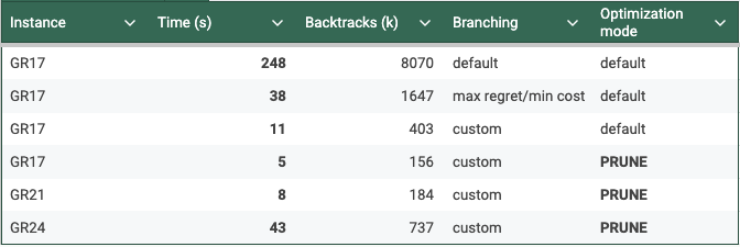
You can find all the corresponding code here.

There are of course many other tracks that we could explore to improve these results:

• design a redundant constraint for the total cost
• improve the branching by exploring new heuristics
• use a different consistency algorithm (NuCS comes with shaving)
• compute lower and upper bounds using other techniques

The travelling salesman problem has been the subject of extensive study and an abundant literature. In this article, we hope to have convinced the reader that it is possible to find optimal solutions to medium-sized problems in a very short time, without having much knowledge of the travelling salesman problem.

Some useful links to go further with NuCS:

• the source code: https://github.com/yangeorget/nucs
• the documentation: https://nucs.readthedocs.io/en/latest/index.html
• the Pip package: https://pypi.org/project/NUCS/

If you enjoyed this article about NuCS, please clap 50 times !

---

How to Tackle an Optimization Problem with Constraint Programming was originally published in Towards Data Science on Medium, where people are continuing the conversation by highlighting and responding to this story.