Calibrating Marketing Mix Models In Python

Part 2 of a hands-on guide to help you master MMM in pymc

What is this series about?

Welcome to part 2 of my series on marketing mix modeling (MMM), a hands-on guide to help you master MMM. Throughout this series, we’ll cover key topics such as model training, validation, calibration and budget optimisation, all using the powerful pymc-marketing python package. Whether you’re new to MMM or looking to sharpen your skills, this series will equip you with practical tools and insights to improve your marketing strategies.

If you missed part 1 check it out here:

Mastering Marketing Mix Modelling In Python

Introduction

In the second instalment of this series we will shift our focus to calibrating our models using informative priors from experiments:

• Why is it important to calibrate marketing mix models?
• How can we use Bayesian priors to calibrate our model?
• What experiments can we run to inform our Bayesian priors?

We will then finish off with a walkthrough in Python using the pymc-marketing package to calibrate the model we built in the first article.

The full notebook can be found here:

pymc_marketing/notebooks/2. calibrating marketing mix models (MMM) in python.ipynb at main · raz1470/pymc_marketing

1.0 Calibrating marketing mix models

Marketing mix modelling (MMM) is a statistical technique used to estimate the impact of various marketing channels (such as TV, social media, paid search) on sales. The goal of MMM is to understand the return on investment (ROI) of each channel and optimise future marketing spend.

There are several reasons why we need to calibrate our models. Before we get into the python walkthrough let’s explore them a bit!

1. 1 Why is it important to calibrate marketing mix models?

Calibrating MMM is crucial because, while they provide valuable insights, they are often limited by several factors:

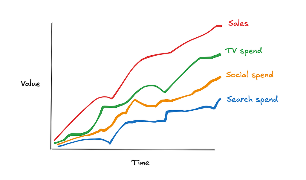
• Multi-collinearity: This occurs when different marketing channels are highly correlated, making it difficult to distinguish their individual effects. For example, TV and social may run simultaneously, causing overlap in their impacts. Calibration helps untangle the effects of these channels by incorporating additional data or constraints.
• Unobserved confounders: MMM models rely on observed data, but they may miss important variables that also affect both marketing and sales, such as seasonality or changes in market demand. Calibration can help adjust for these unobserved confounders.

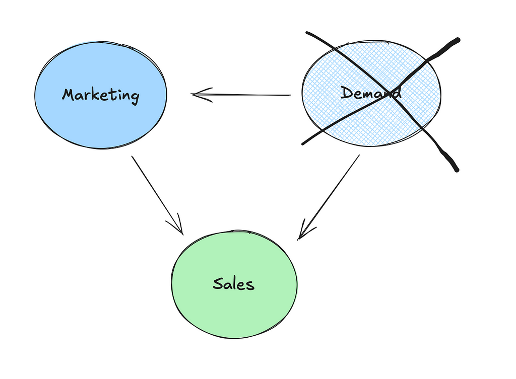
• Re-targeting bias: Have you ever visited a website for a product and then found that all of your social media platforms are now suddenly “coincidently” showing you ads for that product? This isn’t a coincidence, it’s what we call retargeting and it can be effective. However, a number of prospects who get retargeted and then go on to purchase would have anyway!

Without proper calibration, these issues can lead to inaccurate estimates of marketing channel performance, resulting in poor decision-making on marketing spend and strategy.

1.2 How can we use Bayesian priors to calibrate our models?

In the last article we talked about how Bayesian priors represent our initial beliefs about the parameters in the model, such as the effect of TV spend on sales. We also covered how the default parameters in pymc-marketing were sensible choices but weakly informative. Supplying informative priors based on experiments can help calibrate our models and deal with the issues raised in the last section.

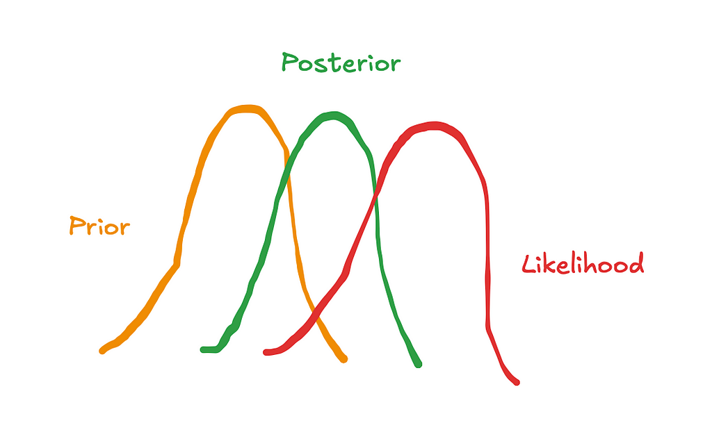
There are a couple of ways in which we can supply priors in pymc-marketing:

• Change the default saturation_beta priors directly like in the example below using a truncated normal distribution to enforce positive values:

model_config = {
    'intercept': Prior("Normal", mu=0, sigma=2),
    'likelihood': Prior("Normal", sigma=Prior("HalfNormal", sigma=2)),
    'gamma_control': Prior("Normal", mu=0, sigma=2, dims="control"),
    'gamma_fourier': Prior("Laplace", mu=0, b=1, dims="fourier_mode"),
    'adstock_alpha': Prior("Beta", alpha=1, beta=3, dims="channel"),
    'saturation_lam': Prior("Gamma", alpha=3, beta=1, dims="channel"),
    'saturation_beta': Prior("TruncatedNormal", mu=[0.02, 0.04, 0.01], lower=0, sigma=0.1, dims=("channel"))
}

mmm_with_priors = MMM(
    model_config=model_config,    
    adstock=GeometricAdstock(l_max=8),
    saturation=LogisticSaturation(),
    date_column=date_col,
    channel_columns=channel_cols,
    control_columns=control_cols,
)

• Use the add_lift_test_measurements method, which adds a new likelihood term to the model which helps calibrate the saturation curve (don’t worry, we will cover this in more detail in the python walkthrough):

lift_test – Open Source Marketing Analytics Solution

What if you aren’t comfortable with Bayesian analysis? Your alternative is running a constrained regression using a package like cvxpy. Below is an example of how you can do that using upper and lower bounds for the coefficients of variables:

import cvxpy as cp

def train_model(X, y, reg_alpha, lower_bounds, upper_bounds):
    """
    Trains a linear regression model with L2 regularization (ridge regression) and bounded constraints on coefficients.

    Parameters:
    -----------
    X : numpy.ndarray or similar
        Feature matrix where each row represents an observation and each column a feature.
    y : numpy.ndarray or similar
        Target vector for regression.
    reg_alpha : float
        Regularization strength for the ridge penalty term. Higher values enforce more penalty on large coefficients.
    lower_bounds : list of floats or None
        Lower bounds for each coefficient in the model. If a coefficient has no lower bound, specify as None.
    upper_bounds : list of floats or None
        Upper bounds for each coefficient in the model. If a coefficient has no upper bound, specify as None.

    Returns:
    --------
    numpy.ndarray
        Array of fitted coefficients for the regression model.

    Example:
    --------
    >>> coef = train_model(X, y, reg_alpha=1.0, lower_bounds=[0.2, 0.4], upper_bounds=[0.5, 1.0])
    
    """

    coef = cp.Variable(X.shape[1])
    ridge_penalty = cp.norm(coef, 2)
    objective = cp.Minimize(cp.sum_squares(X @ coef - y) + reg_alpha * ridge_penalty)
    
    # Create constraints based on provided bounds
    constraints = (
        [coef[i] >= lower_bounds[i] for i in range(X.shape[1]) if lower_bounds[i] is not None] +
        [coef[i] <= upper_bounds[i] for i in range(X.shape[1]) if upper_bounds[i] is not None]
    )

    # Define and solve the problem
    problem = cp.Problem(objective, constraints)
    problem.solve()
    
    # Print the optimization status
    print(problem.status)
    
    return coef.value

1.3 What experiments can we run to inform our Bayesian priors?

Experiments can provide strong evidence to inform the priors used in MMM. Some common experiments include:

• Conversion lift tests — These tests are often run on platforms like Facebook, YouTube, Snapchat, TikTok and DV360, where users are randomly split into a test and control group. The test group is exposed to the marketing campaign, while the control group is not. The difference in conversion rates between the two groups informs the actual lift attributable to the channel.
• Geo-lift tests — In a geo-lift test, marketing efforts are turned off in certain geographic regions while continuing in others. By comparing the performance in test and control regions, you can measure the incremental impact of marketing in each region. The CausalPy python package has an easy to use implementation which is worth checking out:

Bayesian geolift with CausalPy – CausalPy 0.4.0 documentation

• Switch-back testing — This method involves quickly switching marketing campaigns on and off over short intervals to observe changes in consumer behavior. It’s most applicable to channels with an immediate impact, like paid search.

By using these experiments, you can gather strong empirical data to inform your Bayesian priors and further improve the accuracy and calibration of your Marketing Mix Model.

2.0 Python walkthrough

Now we understand why we need to calibrate our models, let’s calibrate our model from the first article! In this walkthrough we will cover:

• Simulating data
• Simulating experimental results
• Pre-processing the experimental results
• Calibrating the model
• Validating the model

2.1 Simulating data

We are going to start by simulating the data used in the first article. If you want to understand more about the data-generating-process take a look at the first article where we did a detailed walkthrough:

Mastering Marketing Mix Modelling In Python

When we trained the model in the first article, the contribution of TV, social, and search were all overestimated. This appeared to be driven by the demand proxy not contributing as much as true demand. So let’s pick up where we left off and think about running an experiment to deal with this!

2.2 Simulating experimental results

To simulate some experimental results, we write a function which takes in the known parameters for a channel and outputs the true contribution for the channel. Remember, in reality we would not know these parameters, but this exercise will help us understand and test out the calibration method from pymc-marketing.

def exp_generator(start_date, periods, channel, adstock_alpha, saturation_lamda, beta, weekly_spend, max_abs_spend, freq="W"):
    """
    Generate a time series of experiment results, incorporating adstock and saturation effects.

    Parameters:
    ----------
    start_date : str or datetime
        The start date for the time series.
    periods : int
        The number of time periods (e.g. weeks) to generate in the time series.
    channel : str
        The name of the marketing channel.
    adstock_alpha : float
        The adstock decay rate, between 0 and 1..
    saturation_lamda : float
        The parameter for logistic saturation.
    beta : float
        The beta coefficient.
    weekly_spend : float
        The weekly raw spend amount for the channel.
    max_abs_spend : float
        The maximum absolute spend value for scaling the spend data, allowing the series to normalize between 0 and 1.
    freq : str, optional
        The frequency of the time series, default is 'W' for weekly. Follows pandas offset aliases
    Returns:
    -------
    df_exp : pd.DataFrame
        A DataFrame containing the generated time series with the following columns:
        - date : The date for each time period in the series.
        - {channel}_spend_raw : The unscaled, raw weekly spend for the channel.
        - {channel}_spend : The scaled channel spend, normalized by `max_abs_spend`.
        - {channel}_adstock : The adstock-transformed spend, incorporating decay over time based on `adstock_alpha`.
        - {channel}_saturated : The adstock-transformed spend after applying logistic saturation based on `saturation_lamda`.
        - {channel}_sales : The final sales contribution calculated as the saturated spend times `beta`.

    Example:
    --------
    >>> df = exp_generator(
    ...     start_date="2023-01-01",
    ...     periods=52,
    ...     channel="TV",
    ...     adstock_alpha=0.7,
    ...     saturation_lamda=1.5,
    ...     beta=0.03,
    ...     weekly_spend=50000,
    ...     max_abs_spend=1000000
    ... )

    """
    # 0. Create time dimension
    date_range = pd.date_range(start=start_date, periods=periods, freq=freq)
    df_exp = pd.DataFrame({'date': date_range})

    # 1. Create raw channel spend
    df_exp[f"{channel}_spend_raw"] = weekly_spend

    # 2. Scale channel spend
    df_exp[f"{channel}_spend"] = df_exp[f"{channel}_spend_raw"] / max_abs_spend

    # 3. Apply adstock transformation
    df_exp[f"{channel}_adstock"] = geometric_adstock(
        x=df_exp[f"{channel}_spend"].to_numpy(),
        alpha=adstock_alpha,
        l_max=8, normalize=True
    ).eval().flatten()

    # 4. Apply saturation transformation
    df_exp[f"{channel}_saturated"] = logistic_saturation(
        x=df_exp[f"{channel}_adstock"].to_numpy(),
        lam=saturation_lamda
    ).eval()

    # 5. Calculate contribution to sales
    df_exp[f"{channel}_sales"] = df_exp[f"{channel}_saturated"] * beta
    
    return df_exp

Below we use the function to create results for an 8 week lift test on TV:

# Set parameters for experiment generator
start_date = "2024-10-01"
periods = 8
channel = "tv"
adstock_alpha = adstock_alphas[0]
saturation_lamda = saturation_lamdas[0]
beta = betas[0]
weekly_spend = df["tv_spend_raw"].mean()
max_abs_spend = df["tv_spend_raw"].max()

df_exp_tv = exp_generator(start_date, periods, channel, adstock_alpha, saturation_lamda, beta, weekly_spend, max_abs_spend)

df_exp_tv

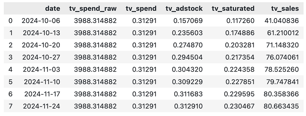
Even though we spend the same amount on TV each week, the contribution of TV varies each week. This is driven by the adstock effect and our best option here is to take the average weekly contribution.

weekly_sales = df_exp_tv["tv_sales"].mean()

weekly_sales

2.3 Pre-processing the experimental results

Now we have collected the experimental results, we need to pre-process them to get them into the required format to add to our model. We will need to supply the model a dataframe with 1 row per experiment in the following format:

• channel: The channel that was tested
• x: Pre-test channel spend
• delta_x: Change made to x
• delta_y: Inferred change in sales due to delta_x
• sigma: Standard deviation of delta_y

We didn’t simulate experimental results with a measure of uncertainty, so to keep things simple we set sigma as 5% of lift.

df_lift_test = pd.DataFrame({
    "channel": ["tv_spend_raw"],
    "x": [0],
    "delta_x": weekly_spend,
    "delta_y": weekly_sales,
    "sigma": [weekly_sales * 0.05],
    }
)

df_lift_test

In terms of sigma, ideally you would have a measure of uncertainty for your results (which you could get from most conversion lift or geo-lift tests).

2.4 Calibrating the model

We are now going to re-train the model from the first article. We will prepare the training data in the same way as last time by:

• Splitting data into features and target.
• Creating indices for train and out-of-time slices — The out-of-time slice will help us validate our model.

# set date column
date_col = "date"

# set outcome column
y_col = "sales"

# set marketing variables
channel_cols = ["tv_spend_raw",
                "social_spend_raw",
                "search_spend_raw"]

# set control variables
control_cols = ["demand_proxy"]

# create arrays
X = df[[date_col] + channel_cols + control_cols]
y = df[y_col]

# set test (out-of-sample) length
test_len = 8

# create train and test indexs
train_idx = slice(0, len(df) - test_len)
out_of_time_idx = slice(len(df) - test_len, len(df))

Then we load the model which we saved from the first article and re-train the model after adding the experimental results:

mmm_default = MMM.load("./mmm_default.nc")
mmm_default.add_lift_test_measurements(df_lift_test)
mmm_default.fit(X[train_idx], y[train_idx])

We won’t focus on the model diagnostics this time round, but you can check out the notebook if you would like to go through it.

2.5 Validating the model

So let’s assess how our new model compares to the true contributions now. Below we inspect the true contributions:

channels = np.array(["tv", "social", "search", "demand"])

true_contributions = pd.DataFrame({'Channels': channels, 'Contributions': contributions})
true_contributions= true_contributions.sort_values(by='Contributions', ascending=False).reset_index(drop=True)
true_contributions = true_contributions.style.bar(subset=['Contributions'], color='lightblue')

true_contributions

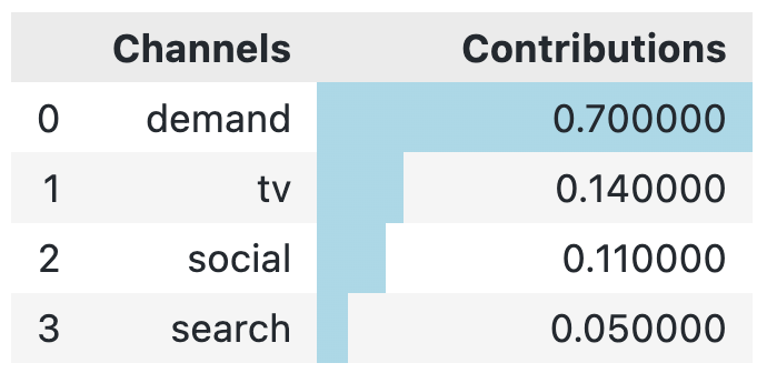
When we compare the true contributions to our new model, we see that the contribution of TV is now very close (and much closer than the model from our first article where the contribution was 24%!).

mmm_default.plot_waterfall_components_decomposition(figsize=(10,6));

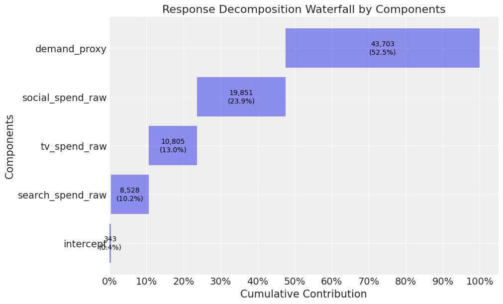
The contribution for search and social is still overestimated, but we could also run experiments here to deal with this.

Closing thoughts

Today we showed you how we can incorporate priors using experimental results. The pymc-marketing package makes things easy for the analyst running the model. However, don’t be fooled….There are still some major challenges on your road to a well calibrated model!

Logistical challenges in terms of constraints around how many geographic regions vs channels you have or struggling to get buy-in for experiments from the marketing team are just a couple of those challenges.

One thing worth considering is running one complete blackout on marketing and using the results as priors to inform demand/base sales. This helps with the logistical challenge and also improvs the power of your experiment (as the effect size increases).

I hope you enjoyed the second instalment! Follow me if you want to continue this path towards mastering MMM— In the next article we will start to think about dealing with mediators (specifically paid search brand) and budget optimisation.

Calibrating Marketing Mix Models In Python was originally published in Towards Data Science on Medium, where people are continuing the conversation by highlighting and responding to this story.