Building an Explainable Reinforcement Learning Framework

Explainable Results Through Symbolic Policy Discovery

Symbolic genetic algorithms, action potentials, and equation trees

We’ve learned to train models that can beat world champions at a games like Chess and Go, with one major limitation: explainability. Many methods exist to create a black-box model that knows how to play a game or system better than any human, but creating a model with a human-readable closed-form strategy is another problem altogether.

The potential upsides of being better at this problem are plentiful. Strategies that humans can quickly understand don’t stay in a codebase — they enter the scientific literature, and perhaps even popular awareness. They could contribute a reality of augmented cognition between human and computer, and reduce siloing between our knowledge as a species and the knowledge hidden, and effectively encrypted deep in a massive high-dimensional tensors.

But if we had more algorithms to provide us with such explainable results from training, how would we encode them in a human-readable way?

One of the most viable options is the use of differential equations (or difference equations in the discrete case). These equations, characterized by their definition of derivatives, or rates of change of quantities, give us an efficient way to communicate and intuitively understand the dynamics of almost any system. Here’s a famous example that relates the time and space derivatives of heat in a system:

In fact, work has been done in the way of algorithms that operate to evolve such equations directly, rather than trying to extract them (as knowledge) from tensors. Last year I authored a paper which detailed a framework for game theoretic simulations using dynamics equation which evolve symbol-wise via genetic algorithms. Another paper by Chen et al. presented work on a symbolic genetic algorithm for discovering partial differential equations which, like the heat equation, describe the dynamics of a physical system. This group was able to mine such equations from generated datasets.

But consider again the game of Chess. What if our capabilities in the computational learning of these equations were not limited to mere predictive applications? What if we could use these evolutionary techniques to learn optimal strategies for socioeconomic games in the real world?

In a time where new human and human-machine relationships, and complex strategies, are entering play more quickly than ever, computational methods to find intuitive and transferable strategic insight have never been more valuable. The opportunities and potential threats are both compelling and overwhelming.

Let’s Begin

All Python code discussed in this article are accessible in my running GitHub repo for the project: https://github.com/dreamchef/abm-dynamics-viz.

In a recent article I wrote about simulating dynamically-behaving agents in a theoretic game. As much as I’d like to approach such multi-agent games using symbolic evolution, it’s wise to work atomically, expand our scope, and take advantage of some previous work. Behind the achievements of groups like DeepMind in creating models with world-class skill at competitive board games is a sub-discipline of ML: reinforcement learning. In this paradigm, agents have an observation space (variables in their environment which they can measure and use as values), an action space (ways to interact with or move/change in the environment), and a reward system. Over time through experimentation, the reward dynamics allow them to build a strategy, or policy, which maximizes reward.

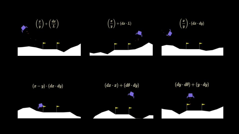
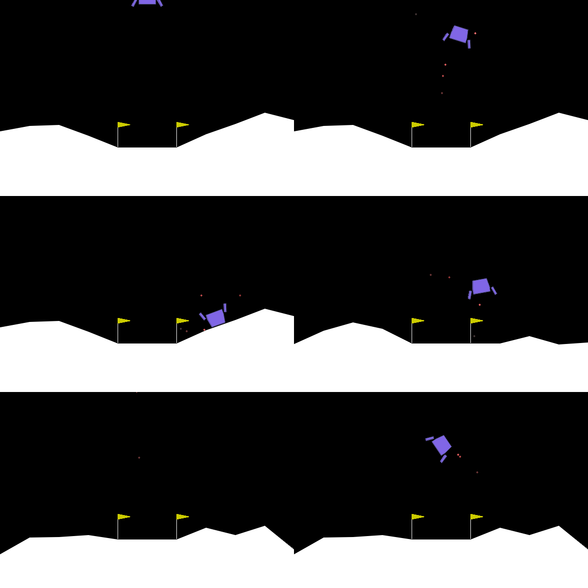
We can apply our symbolic genetic algorithms to some classic reinforcement learning problems in order to explore and fine tune them. The Gymnasium library provides a collection of games and tasks perfect for reinforcement learning experiments. One such game which I determined to be well-suited to our goals is “Lunar Lander”.

The game is specified as follows:

• Observation space (8): x,y position, x, y velocity, angle, angular velocity, left, right foot touching ground. Continuous.
• Action space (4): no engine, bottom, left, right engine firing. Discrete.

Learning Symbolic Policies for the Lander Task

You might have noticed that while the variables like velocity and angle are continuous, action space is discrete. So how do we define a function that takes continuous inputs and outputs, effectively, a classification? In fact this is a well-known problem and the common approach is using an Action Potential function.

Action Potential Equation

Named after the neurological mechanism, which operates as a threshold, a typical Action Potential function calculates a continuous value from the inputs, and outputs:

• True output if the continuous value is at or above a threshold.
• False is the output is below.

In our problem, we actually need to get a discrete output in 4 possible values. We could carefully consider the dynamics of the task in devising this system, but I chose a naive approach, as a semi-adversarial effort to put more pressure on our SGA algorithm to ultimately shine through. It uses the general intuition that near the target probably means we shouldn’t use the side thrusters as much:

            
def potential_to_action(potential):

    if abs(potential-0) < 0.5:
        return 0
    
    elif abs(potential-0) < 1:
        return 2

    elif potential < 0:
        return 1
    
    else:
        return 3

With this figured out, let’s make a roadmap for the rest of our journey. Our main tasks will be:

1. Evolutionary structure in which families and generations of equations can exist and compete.
2. Data structure to store equations (which facilitates their genetic modification).
3. Symbolic mutation algorithm— how and what will we mutate?
4. Selection method — which and how many candidates will we bring to the next round?
5. Evaluation method — how will we measure the fitness of an equation?

Evolutionary Structure

We start by writing out the code on a high-level and leaving some of the algorithm implementations for successive steps. This mostly takes the form of an array where we can store the population of equations and a main loop that evolves them for the specified number of generations while calling the mutation, selection/culling, and testing algorithms.

We can also define a set of parameters for the evolutionary model including number of generations, and specifying how many mutations to create and select from each parent policy.

The following code

last_gen = [F]

for i in range(GENS):
    next_gen = []

    for policy in last_gen:
        batch = cull(mutants(policy))

        for policy in batch:
            next_gen.append(policy) 
    
    last_gen = next_gen

Finally it selects the best-performing policies, and validates them using another round of testing (against Lunar Lander simulation rounds):

last_gen.sort(key=lambda x: x['score'])

final_cull = last_gen [-30:]

for policy in final_cull:

    policy['score'] = score_policy(policy,ep=7)

final_cull.sort(key=lambda x: x['score'])

print('Final Popluation #:',len(last_gen))

for policy in final_cull:
    print(policy['AP'])
    print(policy['score'])
    print('-'*20)

env.close()

Data Structure to Store Equations

We start by choosing a set of binary and unary operators and operands (from the observation space) which we represent and mutate:

BIN_OPS = ['mult','add','sub', 'div']
UN_OPS = ['abs','exp','log','sqrt','sin','cos']
OPNDS = ['x','y','dx','dy','angle','dangle','L','R']

Then we borrow from Chen et al. the idea of encoding equations int the form of trees. This will allow us to iterate through the equations and mutate the symbols as individual objects. Specifically I chose to do using nested arrays the time being. This example encodes x*y + dx*dy:

F = {'AP': ['add', 
                ['mult','x','y'],
                ['mult','dx','dy']],
        'score': 0
        }

Each equation includes both the tree defining its form, and a score object which will store its evaluated score in the Lander task.

Symbolic Mutation Algorithm

We could approach the mutation of algorithms in a variety of ways, depending on our desired probability distribution for modifying different symbols in the equations. I used a recursive approach where at each level of the tree, the algorithm randomly chooses a symbol, and in the case of a binary operator, moves down to the next level to choose again.

The following main mutation function accepts a source policy and outputs an array including the unchanged source and mutated policies.

def mutants(policy, sample=1):
    children = [policy]
    mutation_target = policy

    for i in range(REPL):
        new_policy = copy.deepcopy(policy)
        new_policy['AP'] = mutate_recursive(new_policy['AP'])
        children.append(new_policy)

    return children

This helper function contains recursive algorithm:

def mutate_recursive(target, probability=MUTATE_P):

    # Recursive case
    if isinstance(target, list):
      random_element = random.choice(range(len(target)))
      target[random_element] = mutate_recursive(target[random_element])
      return target

    # Base cases
    elif(target in BIN_OPS):
      new = random.choice(BIN_OPS)
      return new
    
    elif(target in UN_OPS):
      new = random.choice(UN_OPS)
      return new
    
    elif(target in OPNDS):
      new = random.choice(OPNDS)
      return new

Selection Method

Selecting the best policies will involve testing them to get a score and then deciding on a way to let them compete and progress to further stages of evolution. Here I used an evolutionary family tree structure in which each successive generation in a family, or batch (e.g. the two on the lower left), contains children with one mutation that differentiates them from the parent.

                +----------+
                | x + dy^2 |
                +----------+
                     |
          +----------+----------+
          |                     |
     +----v----+           +----v----+
     | y + dy^2|           | x / dy^2|
     +---------+           +---------+
          |                      |
     +----+----+            +----+-----+
     |         |            |          |
 +---v--+-+ +--v---+-+   +--v-----+ +--v-----+
 |y - dy^2| |y - dy^2|   |x / dx^2| |y - dy^3|
 +--------+ +--------+   +--------+ +--------+

After scoring of the equations, each batch of equations is ranked and the best N are kept in the running, while the rest are discarded:

def cull(batch):

    for policy in batch[1:]:
        policy['score'] = score_policy(policy)

    batch.sort(key=lambda x: x['score'], reverse=True)

    return batch[:CULL]

Scoring Methods Through Simulation Episodes

To decide which equations encode the best policies, we use the Gymnasium framework for the Lunar Lander task.

def score_policy(policy, ep=10, render=False):
    observation = env.reset()[0]  # Reset the environment to start a new episode
    total_reward = 0
    sample = 0

    for episode in range(ep):
        
        while True:
            if render:
                env.render()
                
            values = list(observation)
            values =    {'x': values[0],
            'y': values[1],
            'dx': values[2],
            'dy': values[3],
            'angle': values[4],
            'dangle': values[5],
            'L': values[6],
            'R': values[7]
            }

            potential = policy_compute(policy['AP'], values)
            action = potential_to_action(potential)

            sample += 1

            observation, reward, done, info = env.step(action)[:4]
            total_reward += reward

            if done:  # If the episode is finished
                break
    
    return total_reward/EPISODES

The main loop for scoring runs the number of episodes (simulation runs) specified, and in each episode we see the fundamental reinforcement learning paradigm.

From a starting observation, the information is used to compute an action via our method, the action interacts with the environment, and the observation for the next step is obtained.

Since we store the equations as trees, we need a separate method to compute the potential from this form. The following function uses recursion to obtain a result from the encoded equation, given the observation values:

def policy_compute(policy, values):

    if isinstance(policy, str):
        if policy in values:
            return values[policy]
        else:
            print('ERROR')
        
    elif isinstance(policy, list):
        operation = policy[0]
        branches = policy[1:]

        if operation in BIN_OPS:

            if len(branches) != 2:
                raise ValueError(f"At {policy}, Operation {operation} expects 2 operands, got {len(branches)}")

            operands = [operand for operand in branches]
            
            left = policy_compute(operands[0], values)
            right = policy_compute(operands[1], values)

            if operation == 'add':
                return left + right
            elif operation == 'sub':
                return left - right
            elif operation == 'mult':
                if left is None or right is None:
                    print('ERROR: left:',left,'right:',right)
                return left * right
            elif operation == 'div':
                if right == 0:
                    return 0
                return left / right

        elif operation in UN_OPS:
            if len(branches) != 1:
                raise ValueError(f"Operation {operation} expects 1 operand, got {len(branches)}")

            operand_value = policy_compute(next(iter(branches)), values)
            
            if operation == 'abs':
                return abs(operand_value)
            elif operation == 'exp':
                return math.exp(operand_value)
            elif operation == 'logabs':
                return math.log(abs(operand_value))
            elif operation == 'sin':
                return math.sin(operand_value)
            elif operation == 'cos':
                return math.cos(operand_value)
            elif operation == 'sqrtabs':
                return math.sqrt(abs(operand_value))
        
        else:
            raise ValueError(f"Unknown operation: {operation}")

    else:
        print('ERROR')
        return 0

The code above goes through each level of the tree, checks if the current symbol is an operand or operator, and according either computes the right/left side recursively or returns back in the recursive stack to do the appropriate operator computations.

Next Steps

This concluded the implementation. In the next article in this series, I’ll be explaining the results of training, motivating changes in the experimental regime, and exploring pathways to expand the training framework by improving the mutation and selection algorithms.

In the meantime, you can access here the slides for a recent talk I gave at the 2024 SIAM Front Range Student Conference at University of Colorado Denver which discussed preliminary training results.

All code for this project is on my repo: https://github.com/dreamchef/abm-dynamics-viz. I’d love to hear what else you may find, or your thoughts on my work, in the comments! Feel free to reach out to me on Twitter and LinkedIn as well.

All images were created by the author except where otherwise noted.

Building an Explainable Reinforcement Learning Framework was originally published in Towards Data Science on Medium, where people are continuing the conversation by highlighting and responding to this story.